PROCEEDINGS OF SPIE
SPIEDigitalLibrary.org/conference-proceedings-of-spieA guide to properly select the
defocusing distance for accurate
solution of transport of intensity
equation while testing aspheric
surfaces
Peyman Soltani, Ahmad Darudi, Ali Reza Moradi, Javad
Amiri, Georges Nehmetallah
Peyman Soltani, Ahmad Darudi, Ali Reza Moradi, Javad Amiri, Georges
Nehmetallah, "A guide to properly select the defocusing distance for accurate
solution of transport of intensity equation while testing aspheric surfaces,"
Proc. SPIE 9868, Dimensional Optical Metrology and Inspection for Practical
Applications V, 986804 (19 May 2016); doi: 10.1117/12.2223208
Event: SPIE Commercial + Scientific Sensing and Imaging, 2016, Baltimore,
Maryland, United States
A Guide to Properly Select the Defocusing Distance for
Accurate Solution of Transport of Intensity Equation
While Testing Aspheric Surfaces
Peyman Soltani1, Ahmad Darudi1, Ali Reza Moradi1,2, Javad Amiri3, Georges Nehmetallah4
1 Physics Department, University of Zanjan, Zanjan, 45195-313, Iran. 2 Department of Physics, Bilkent University, Cankaya, Ankara 06800, Turkey
3 University of Maragheh, Maragheh, Iran.
4 EECS Department, The Catholic University of America, 620 Michigan Av., N.E., Washington DC 20064
ABSTRACT
In this paper, the Transport of Intensity Equation (TIE) for testing of an aspheric surface is verified experimentally. Using simulation, a proper defocus distance ∆𝑧 that leads to an accurate solution of TIE is estimated whenever the conic constant and configuration of the experiment are known. To verify this procedure a non-nulled experiment for testing an aspheric is used. For verification of the solution, the results are compared with the Shack-Hartmann sensor. The theoretical method and experimental results are compared to validate the results.
Keywords: Aspheric, transport of intensity equation,
surface inspection, Shack-Hartmann wavefront sensor
.1.
INTRODUCTION
In optical design, usage of aspheric surfaces reduces the number of optical elements needed in a specific system and hence reduces the overall weight and size of the optical system. Beside some challenges in the manufacturing of aspheric surfaces, the testing of aspheric surfaces is also an ongoing research subject [1-6]. Generally, there is a large deviation in the optical path of the reflection beam from an aspheric surface which makes testing without a null system a difficult task [7]. The well-known non-null methods are stitching and annual subaperture testing [8-13]. Recently, E. Garbusi et al. presented a novel non-null interferometer for the precise measurement of aspheric surfaces using an array of point sources [5]. Pfund et al. implemented the shack-Hartmann method to measure rotationally symmetric aspheres without a null optics [14].
In this paper, we present a method for measuring the convex aspheric surface wavefront based on the transport-of-intensity equation (TIE). This technique suggested originally by Teague [15] and Streibl [16]. In 1993, Roddier et al. made use of this technique for the purpose of testing the optical quality of ground-based telescopes [17,18]. For solving the TIE, many effective numerical methods such as the method based on Green’s function [19], multigrid (MG) [20, 21], and the Zernike polynomial expansion method [22, 23] were presented. Currently, TIE technique is used in different fields of physics such as adaptive optics [24, 25], microscopy [26, 27], optical measuring [28-30], and optical tomography [31-33], just to name a few.
In a typical TIE experiment, intensity distributions are measured at two defocused planes perpendicular to the propagation axis. Their difference is computed and divided by the defocusing distance ∆z separating these two planes, to estimate the intensity derivative along the propagation direction z. Hence, the estimate of the derivative can be written as
.
Δ
2
Δ
,
,
2
Δ
,
,
y)
(x,
z
z
y
x
I
z
y
x
I
z
I
(1)By increasing the defocusing distance ∆z between the two planes, the signal is less affected by measurement noise error. However, the calculation of the derivative becomes less precise. Hence, the distance ∆z has to be correctly estimated to obtain accurate results. In a previous work [34], we presented a theoretical method to accurately estimate the defocusing distance by investigation the error contribution due to Δz in which it is assumed that the radius of curvature (ROC) and conic constant of an aspheric surface is known. We demonstrated that an optimum value for Δz is related to the peak-to-valley (PV) of the phase distribution in which the contribution of piston, tilt, and the quadric term have been removed to accurately estimate the PV [34]. In this study, we demonstrate experimentally how to measure aspheric surfaces of which its conic constant and ROC are known. In order to validate the measurement accuracy, we compare the results obtained by the TIE method with the results obtained by the Shack-Hartmann method (SH), and we show that the results of the two methods are in good agreement with one another.
2. TRANSORT OF INENSITY EQUATION
Consider the Helmholtz equation:
2
k
2
U
(
r
)
0
,
that governs the propagation of the complex plane wave field) exp( ) , , ( ) , , (x yz E x yz jkz
U in free space, where
2 2 2 2 2y
x
denotes the transverse Laplacian operator. In theparaxial approximation, the imaginary part of the Helmholtz equation can lead to the TIE equation [21]:
I
2φ
x
,
y
,
z
I
φ
x
,
y
,
z
,
z
I
k
(2)where k is the wave constant and the complex amplitudeE(x,y,z) can be written as follows:
)).
,
,
(
exp(
)
,
,
(
)
,
,
(
x
y
z
I
x
y
z
j
φ
x
y
z
E
(3)The TIE equation links the axial changes of the spatial intensity (∂I/∂z) to the spatial intensity I(x,y,z) and phase
(x, y, z). The most common technique to solve the TIE is presented by Roddier et al. [17] which is based on Fourier transform iterative method. Assuming the intensity distribution at the pupil plane (z0=0) is constant
I
0
,
and Eq. (2)is converted into a Poison equation [27]:
,
Δ
2
,
,
2S
z
k
z
y
x
φ
(4)where the signal function, 𝑆, is given by:
,
,
Δ
2
,
,
Δ
2
2
Δ
,
,
2
Δ
,
,
0 0 0 0z
z
y
x
I
z
z
y
x
I
z
z
y
x
I
z
z
y
x
I
S
, (5)where
I
x
,
y
,
z
0
Δ
z
2
andI
x
,
y
,
z
0
Δ
z
2
denote the intensity distributions along the z-axis on the underfocus and overfocus planes of the system, respectively and are separated byΔ
z
. Eq. (4) can be solved using the Fourier transform method as:
,
Δ
2
,
,
1 2 2
y xk
k
S
z
k
z
y
x
φ
F
F
(6)where F and
F
1 are the forward and inverse 2D Fourier transform andk
x andk
y are the spatial frequencies in the Fourier domain.3. EXPERIMENTAL SETUP
The TIE approach described in the previous section is used for metrology testing of an aspheric surface. The non-null configuration is used in which the phase aberration of the reflected wave is given by:
CCI
I.I-I)
r
φ
r
φ
r
φ
asph
sph , (7) whereφ
asph
r
is the phase of an aspheric surface defined as:
n i i i asphA
φ
r
r
K
R
R
r
r
φ
1 2 2 2 21
, (8)where R is the radius of curvature at the vertex of the aspheric surface, K is the conic constant,
A
iφ
r
2i are higher order aspheric terms (for simplicity, we assume that the higher order aspheric aberrations are zeros),r
x
2
y
2 is the radial distance from optical axis, andφ
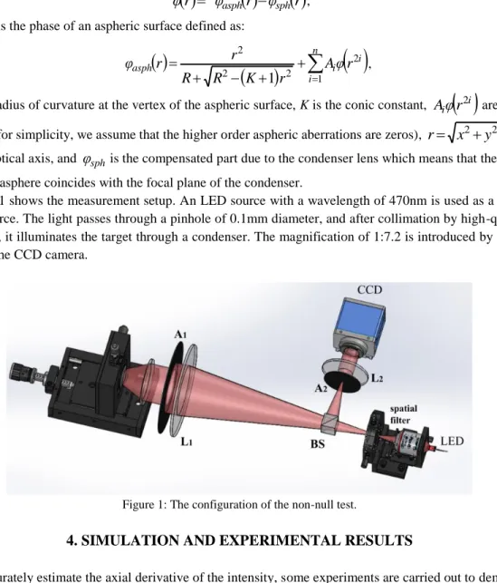
sph is the compensated part due to the condenser lens which means that the center of the curvature of the asphere coincides with the focal plane of the condenser.Figure 1 shows the measurement setup. An LED source with a wavelength of 470nm is used as a low coherent illumination source. The light passes through a pinhole of 0.1mm diameter, and after collimation by high-quality double lens (f=500mm), it illuminates the target through a condenser. The magnification of 1:7.2 is introduced by a collimating lens in front of the CCD camera.
Figure 1: The configuration of the non-null test.
4. SIMULATION AND EXPERIMENTAL RESULTS
To accurately estimate the axial derivative of the intensity, some experiments are carried out to demonstrate that the optimum value of the defocusing distance Δz is related to the peak-to-valley (PV) of the aspheric phase distribution. An aspheric surface of conic constant K=-0.012, radius of curvature R=15 mm, and maximum pupil diameter of 17mm, is used in the experiment. The PV of the phase distribution is controlled by the size of the pupil which is placed before the condenser lens.
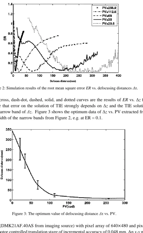
A series of simulations are carried out based on Ref. [34]. The defocusing distance Δz is varied from 1.0 mm to 400/7.2 mm (because of magnification) and for five pupil diameters: [24, 21, 19, 16.8, and 15] mms corresponding to PV: [255.9, 112.6, 68, 37, and 20.6] radians, respectively. In order to quantify the percentage of the error between the predefined wavefront and reconstructed ones the root mean square error is used:
dA
φ
dA
φ
φ
ER
TIE i TIE 2 2 , (9)1A 1.2 1 x PV=256.9 --PVe112.6 - - - PV=68
- PV=35
PV=20.6 :y. 0.6i
0.4w i i xi
0.2 x;
i
-o o 50 100 150 200 250 Detacua d(aance(mml 300 350 350 300 250-200 150 100 50-50 100 150 200 250 300 PV(rad)Figure 2: Simulation results of the root mean square error ER vs. defocusing distances Δz.
In Figure 2 the cross, dash-dot, dashed, solid, and dotted curves are the results of ER vs. Δz for different PVs. From Figure 2, it is clear that error on the solution of TIE strongly depends on Δz and the TIE solution has minimum percentage of error in a narrow band of Δz. Figure 3 shows the optimum data of Δz vs. PV extracted from Figure 2. The error bars illustrate the width of the narrow bands from Figure 2, e.g. at ER = 0.1.
Figure 3: The optimum value of defocusing distance Δz vs. PV.
A CCD camera (DMK21AF.40AS from imaging source) with pixel array of 640×480 and pixel size x=5.6µm
is mounted on a stepper motor controlled translation stage of incremental accuracy of 0.048 mm. An x-y manual translation stage and a tip/tilt mount are also used to adjust the position of the aspheric surface.
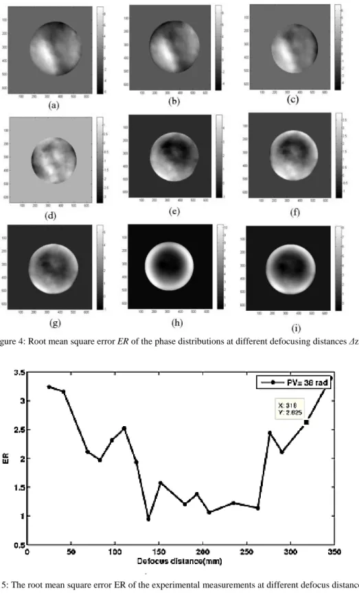
The intensity distributions are recorded on opposite sides of the virtual image plane starting from a distance of 3.5mm to 48 mm with increment of 2.5 mm. The PV values have been estimated from phase distribution obtained from the simulation (Eq. (8)). Figure 4 shows the error in phase distribution at different defocusing distances.
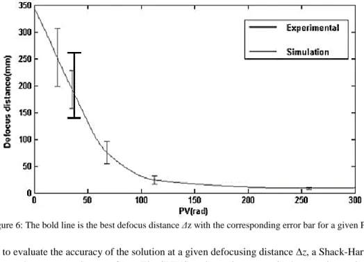
Figure 5 shows the root means square error ER of phase retrieval calculated by substituting the theoretical phase distribution (calculated using known asphere parameters) by the phase distribution obtained from solving the TIE. Figure 6 shows the best defocus distance Δz with the corresponding error bar for a given PV.
m S m IP (d) SA UO 03 m 30 m (e) mG tm ID lm IZ (g) Op (h) 9m m4 im m lm 0o Ra (C) 40 m m mO Im 5m 03
(fl
fm mn m Im SOD mo (1) 3.5 3 2.5 ¢ 2 w 1.5 1 .. 0.50 50 100 150 200 250 Defocus dtsuance(mm) 300 350Figure 4: Root mean square error ER of the phase distributions at different defocusing distances Δz.
350 300 E 250 C 100 50 00 Experimental Simulation 50 100 150 200 250 300 PV(rati} 30 20 10 PV(rad) o -10 -20 20 lo ° o Spots number 10 15 20 25
Figure 6: The bold line is the best defocus distance Δz with the corresponding error bar for a given PV.
In order to evaluate the accuracy of the solution at a given defocusing distance Δz, a Shack-Hartmann wavefront sensor (SHWS) is used to measure the wavefront. The SHWS replaces the camera in the experimental setup in Figure 1. The SHWS sensor consists of camera model MLA150-7AR from Thorlabs and a 50×50 lenslet array of overall size 10×10 mm. The focal length of each lenslet is f= 6.7 mm and the lenslet diameter is 150μm.
The centroids of the recorded spots on the CCD are analyzed to calculate the slope information by comparing the SH grid coordinates of the object beam with that of the reference beam. Figure 7 shows one of the reconstructed phase distributions using the SHWS. The results obtained from the SHWS are in excellent agreement with those measured by the TIE method.
Figure 7: The phase distribution calculated using the SHWS.
5. CONCLUSION
In this paper, TIE is experimentally verified as a tool to be used for testing of an aspheric surface. Using simulation, a proper defocus distance ∆𝑧 is estimated leading to an accurate solution of TIE, whenever the conic constant and configuration of the experiment are known. A non-nulled experiment for testing an aspheric was used to verify this TIE technique. For verification of the solution, a Shack-Hartmann sensor was also employed.
REFERENCES
[1] Wyant, J. C. and Bennett, V. P., “Using computer generated holograms to test aspheric wavefronts,” Appl. Opt. 11(12), 2833-2839 (1972).
[2] Ono A. and. Wyant, J. C, “Aspherical mirror testing using a CGH with small errors,” Appl. Opt. 24(4), 560-563 (1985). [3] Burge, J. H., “Fizeau interferometry for large convex surfaces,” Proc. SPIE 2536, Optical manufacturing and testing, 127-138
(1995).
[4] Kim, T., Burge, J. H., Lee, Y., and Kim, S., “Null test for a highly paraboloidal mirror,” Appl. Opt. 43(18), 3614-3618 (2004). [5] Garbusi, E., Pruss, C., and Osten, W., “Interferometer for precise and flexible asphere testing,” Opt. Lett. 33(24), 2973-2975
(2008).
[6] Kino, M. and Kurita, M., “Interferometric testing for off-axis aspherical mirrors with computer generated holograms,” Opt. Appl.
51(19),4291-4297 (2012).
[7] Malacara, D., [Optical shop testing] Third Edition Wiley, New York (2007).
[8] Murphy, P., Fleig, J., Forbes, G., Miladinovic, D., DeVries, G., O' Donohue, S., “Subaperture stitching interferometry for testing mild aspheres,” Proc. SPIE 6293, 62930J (2006).
[9] Kuchel, M. F., “Absolute measurement of rotationally symmetrical aspheric surfaces,” OSA Topical Meeting on Optical Fabrication and Testing, Rochester, USA, OFTuB5 (2006).
[10] Wen, Y., Cheng, H., Tam, H.Y., and Zhou, D., “Modified stitching algorithm for annular subaperture stitching interferometry for aspheric surfaces,” Appl. Opt. 23(52), 5686-5694 (2013).
[11] Greivenkamp, J. E. and Gappinger, R. O., “Design of a non-null interferometer for aspheric wave fronts,” Appl. Opt. 43(27), 5143–5151 (2004).
[12] Liu, Y.-M., Lawrence, G. N., and Koliopoulos, C. L., “Subaperture testing of aspheres with annular zones,” Appl. Opt. 27(21), 4504–4513 (1988).
[13] Melozzi, M., Pezzati, L., and Mazzoni, A., “Testing aspheric surfaces using multiple annular interferograms,” Opt. Eng. 32(5), 1073–1079 (1993).
[14] Pfund, J., Lindlein, N., and Schwider J., “Non-null testing of rotationally symmetric aspheres: a systematic error assessment,” Appl. Opt. 40(4), 439-446 (2001).
[15] Teague, M.R., “Irradiance moments: their propagation and use for unique retrieval of phase,” J. Opt. Soc. Am. 72, 1199-1209 (1982).
[16] Streibl, N., “Phase imaging by the transport equation of intensity,” Opt. Comm. 49, 6–10 (1984).
[17] Roddier, F. and Roddier, C., “Wavefront reconstruction using iterative Fourier transforms,” Appl. Opt. 30(11),1325-1327 (1991). [18] Roddier, C. and Roddier, F., “Wave-front reconstruction from defocused images and the testing of ground-based optical
telescopes,” J. Opt. Soc. Am. A 10, 2277–2287 (1993).
[19] Teague, M.R., “Deterministic phase retrieval: a Green’s function solution,” J. Opt. Soc. Am. 73, 1434–1441 (1983).
[20] Allen, L. J. and. Oxley, M. P., “Phase retrieval from series of images obtained by defocus variation,” Opt. Comm. 199(1-4), 65– 75 (2001).
[21] Xiao, W., Heng, M., and Dazun, Z., “Phase retrieval based on intensity transport equation,” Acta Opt. Sin. 27, 2117–2122 (2007). [22] Gureyev, T. E., Roberts, A., and Nugent, K. A., “Phase retrieval with the transport-of-intensity equation: matrix solution with use
of Zernike polynomials,” J. Opt. Soc. Am. 12(9), 1932–1941 (1995).
[23] Pinhasi, S. V., Alimi, R., Perelmutter, L., and Eliezer, S., “Topography retrieval using different solutions of the transport intensity equation,” J. Opt. Soc. Am. A 27(10), 2285–2292 (2010).
[24] Orlav, V., Luna, E., Orlova, E., “Optimal defocus distance for testing the 2.1 m telescope at San Pedro Martir,” Appl. Opt. 44(25), 5169–5172 (2005).
[25] Pinhasi, S. V., Alimi, R., Perelmutter, L., and Eliezer, S., “Topography retrieval using different solutions of the transport intensity equation,” J. Opt. Soc. Am. A 27(10), 2285–2292 (2010).
[26] Bajt, S., Barty, A., Nugent, K.A., McCartney, M., Wall, M., Paganin, D., “Quantitative phase-sensitive imaging in a transmission electron microscope,” Ultramicroscopy 83(1–2) 67–73 (2000).
[27] Frank, J., Matrisch, J., Horstmann, J., Altmeyer, S., and Wernicke, G., “Refractive index determination of transparent samples by noniterative phase retrieval,” Appl. Opt. 50(4), 427–433 (2011).
[28] Darudi, A., Shomali, R., Tavassoly, M.T., “Determination of the refractive index profile of a symmetric fiber preform by the transport of intensity equation,” Opt. Laser Technol. 40, 850–853 (2008).
[29] Amiri, J., Darudi, A., Khademi, S., and Soltani, P., “Application of transport of intensity equation in fringe analysis”, Opt. Lett.
39(10), 2864-2867 (2014).
[30] Soltani, P., Moradi, A-R., Darudi, A., Shomali, R., “High resolution optical surface testing using transport of intensity equation”, Proc. SPIE 8785, 8th Iberoamerican Optics Meeting and 11th Latin American Meeting on Optics, Lasers, and Applications, 87851K, November 18 (2013).
[31] Memarzadeh, S., Banerjee, P. P., and Nehmetallah, G., “Noninterferometric tomographic reconstruction of 3D static and dynamic phase and amplitude objects,” Proc. SPIE 9117, Three-Dimensional Imaging, Visualization, and Display, 91170M (2014). [32] Nguyen, T. C., Nehmetallah, G., Darudi, A., and Soltani, P., “3D high speed characterization of phase and amplitude objects using
the transport of intensity equation,” Proc. SPIE 949512, Three-Dimensional Imaging, Visualization, and Display, May 22 (2015). [33] Nguyen, T., Nehmetallah, G., Tran, D., Darudi, A., and Soltani, P., “Fully automated, high speed, tomographic phase object reconstruction using the transport of intensity equation in transmission and reflection configurations,” Applied Optics 54(35), 10443-10453 (2015).
[34] Shomali, R., Darudi, A., Nasiria, S., “Application of irradiance transport equation in aspheric surface testing,” Optik 123, 1282– 1286 (2012).