Quality versus quantity the limited impact of compulsory schooling laws on household financial behavior

(1)

QUALITY VERSUS QUANTITY

THE LIMITED IMPACT OF COMPULSORY SCHOOLING LAWS ON HOUSEHOLD FINANCIAL BEHAVIOR

A Master’s Thesis

by MARIE LEKA

Department of Economics İhsan Doğramaci Bilkent University

Ankara August 2020

(2)

(3)

(4)

The Graduate School of Economics and Social Sciences

of İhsan Doğramacı Bilkent University

by

MARIE LEKA

In Partial Fulfillment of the Requirements for the Degree of MASTER OF ARTS

THE DEPARTMENT OF ECONOMICS İHSAN DOĞRAMACI BİLKENT UNIVERSITY

ANKARA

(5)

(6)

iii

ABSTRACT

Leka, Marie

M.A., Department of Economics

Supervisor: Assist. Prof. Dr. Şaziye Pelin Akyol

August, 2020

The low level of household financial market participation is one of the important puzzles remaining to be solved in modern economics. Yet, we have still to understand its

determinants. We exploit the exogenous variation induced by a change in compulsory schooling laws in Turkey to estimate the impact of compulsory schooling laws on household borrowing and saving decisions. Using Reduced Form regressions, we find that the education reform increased the schooling level of household heads and had a positive impact on households’ propensity to hold savings in bank accounts. However, we do not observe such a relationship in the remaining measures of saving and

borrowing. These results point to a limitation of the impact of policies that only increase the years of schooling on financial market participation, and highlight the importance of the inclusion of financial training in early education curriculums.

Keywords: Compulsory Schooling Law, Financial Markets, Household Data, Reduced

(7)

iv

ÖZET

NİTELİK VE NİCELİK

ZORUNLU EĞİTİM YASALARIN HANEHALKININ FİNANSAL DAVRANIŞI ÜZERİNDEKİ SINIRLI ETKİSİ

Leka, Marie

Yüksek Lisans, İktisat Bölümü

Tez Danışmanı: Dr. Öğr. Üyesi: Şaziye Pelin Akyol

Ağustos, 2020

Hane halkının finansal piyasalara katılımının düşük olması, modern ekonomide

çözülmesi gereken önemli bulmacalardan biridir. Ancak, hala bunu etkileyen faktörleri anlamamız gerekiyor. Zorunlu eğitim yasalarının hanehalkı borçlanması ve tasarruf kararları üzerindeki etkisini tahmin etmek için, Türkiye'deki zorunlu eğitim yasalarındaki bir değişikliğin neden olduğu dışsal değişimlerden yararlanıyoruz. İndirgenmiş Biçim Regresyonu kullanarak, eğitim reformunun hanehalkı reislerinin eğitim seviyesini artırdığını ve hane halklarının banka hesaplarında tasarruf tutma eğilimi üzerinde olumlu bir etkisi olduğunu tespit ettik. Ancak, kalan tasarruf ve borçlanma ölçülerinde böyle bir ilişki gözlemlemiyoruz. Bu sonuçlar, yalnızca eğitim sürelerinin artışina sebep olan politikaların finansal market katılımına etkisinin ciddi bir şekilde sınırlı olduğuna işaret etmekte ve finansal eğitimin erken eğitim müfredatlarına dahil edilmesinin önemini vurgulamaktadır.

Anahtar Kelimeler: Finansal Piyasalar, Hane Verileri, İndirgenmiş Biçim Regresyonu,

(8)

v

ACKNOWLEDGEMENTS

I would like to express the deepest appreciation to my supervisor, Assist. Prof. Dr. Pelin Akyol, for her indispensable guidance not only through my research, but also in

discovering my place in economics. I would like to thank her for believing in me and pushing me to put forth my best effort. I would like to thank my examining committee members, Assoc. Prof. Dr. Çağla Okten and Assist. Prof. Dr. Mürüvvet Büyükboyacı, for their helpful comments. I would be remiss if I did not give my thanks to Assist. Prof. Dr. Banu Demir Pakel for her invaluable support in one of the most crucial parts of my educational experience.

(9)

vi

LIST OF TABLES

Table 1: Descriptive statistics (by treatment status) ... 9

Table 2: Effect of Reform on education ... 14

Table 3: Effect of Reform on spouses’ education ... 15

Table 4: Effect of junior high school completion on household financial behavior ... 16

Table 5: Effect of Reform on household financial behavior... 18

Table 6: Robustness check: bandwidth selection ... 20

Table 7: Robustness check: keeping the 1986 cohort ... 21

Table 8: Effect of placebo Reform on education ... 22

Table 9: Effect of placebo Reform on household financial behavior ... 23

Table 10: Descriptive statistics (by marital status of the household head) ... 32

Table 11: Effect of Reform on individual characteristics ... 33

Table 12: Effect of Reform on household financial behavior (full specification) ... 34

Table 13: Effect of Reform on household financial behavior (controlling for marital status) ... 35

Table 14: Effect of placebo Reform on education (additional years) ... 36

Table 15: Effect of placebo Reform on household financial behavior (additional years) 37 Table 16: Variable definitions ... 38

(11)

viii

LIST OF FIGURES

Figure 1: Proportion of individuals with at least junior high school degree by birth cohort ... 4 Figure 2: Treatment effect on household borrowing and saving measures by birth cohort ... 31 Figure 3: Placebo Treatment effect on junior high school completion by birth cohort .... 31

(12)

1

CHAPTER 1 PRELIMINARIES

1.1 Introduction

The 21st century, among other things, has witnessed a major overhaul of what we consider as the ‘modern’ economy, and the most obvious example of that can be seen in the financial markets: individuals are continuously being presented with new and

complex financial products. This creates a bipolar problem when it comes to making the decision on whether to engage in said financial markets. On one hand, the rapid pace of the technological improvement not only allows for new and exciting financial

instruments to be created steadily, but it also facilitates one’s access to them. On the other, it is becoming increasingly difficult to keep up with the changes. While the navigation of the financial market has always been a task for the more cognitively endowed, the increase in the variety and the speed of transactions has, inadvertently, increased the barriers to entry. One of the ways through which we expect individuals to gain the necessary knowledge to participate in the financial market is schooling.

Education has always been considered a cornerstone of combined micro- and macro-economic policy making. This is not in naught: several studies have found evidence of labor market and other, non-pecuniary, returns to primary or secondary education,

(13)

2

especially when it is the target of institutionally driven policies (Angrist & Krueger, 1991; Oreopoulos, 2006). When it comes to financial behavior, the effect of education is expected to be positive: Agarwal and Mazumder (2013) emphasize the importance of cognitive ability (measured as high math scores) in sound financial decision making. The mathematical and economic training received with schooling can increase relevant cognitive capacity, and thus, the probability of participating in the financial market. In addition, due to its positive effect on earnings, education can increase the probability of participating in the financial market by creating wealth accumulation opportunities (Cooper & Zhu, 2015).

We exploit an exogenous change in compulsory schooling laws to determine the effect of schooling on household financial behavior in a developing country – Turkey. This choice is deliberate, because, while Turkey has a modern financial market, it registers one of the lowest private saving rates among large economies. In 2018, a survey from ING bank found that only 16% of the respondents declared to have any savings, with the majority preferring to keep it ‘under the pillow’, hinting at a low financial market participation rate. To answer our question, we refer to a change in compulsory schooling laws in 1997, which targeted primary education, by increasing mandatory schooling from five to eight years for all those younger than 11 years of age. The new law was enacted swiftly and unexpectedly, thus generating an exogenous increase in schooling for this particular cohort, leaving older ones unaffected. We first look into the effect of this policy change on schooling for the impacted cohort. Then, we examine whether this change had any impact on two main aspects of household financial behavior – borrowing and saving. We use the 2016 Family Structure Survey to estimate the effects of an increase in educational attainment of the household head on household financial market participation. The survey is conducted on a household basis, where members of a household are surveyed privately. Thus, the dataset contains information on each respondents’ individual, familial and educational background, their employment status and overall level of well-being. General questions are asked on each individuals’ financial market participation, and then, a representative is asked to provide detailed information on the household’s financial behavior, which is intended to determine the

(14)

3

existence of debt or savings, their source and the form in which they are kept by the household. We make use of these responses to construct variables of financial market participation, which are divided into two categories: debt-related and saving-related. These variables will determine not only the existence of either household debt or saving, but also whether these activities are performed through a financial intermediary and if so, they report the type of financial instrument/s used by the household. These will be our outcome variables.

Simple correlation would not be useful in unveiling the relationship we are after, as these estimates are likely to suffer from omitted variable bias: unobserved factors, such as ability, motivation or upbringing, may affect both educational attainment and financial behavior. We address the endogeneity of education by using the treatment effect

generated by the Basic Education Program as its proxy: a dummy variable is constructed, which indicates whether the individual has been affected by the law change. The

treatment status will be assigned according to the respondent’s year of birth, with 1986 as the cutoff. The causal nature of the estimates is challenged by the joint decision making one can observe when it comes to household resolutions, due to the fact that the reform may have affected both the household head and their spouse. We limit our analysis to only the effect of household head’s schooling on household financial behavior and use Reduced Form (RF) regressions to make conditional predictions on financial outcomes, given the exogenous variation created by the reform.

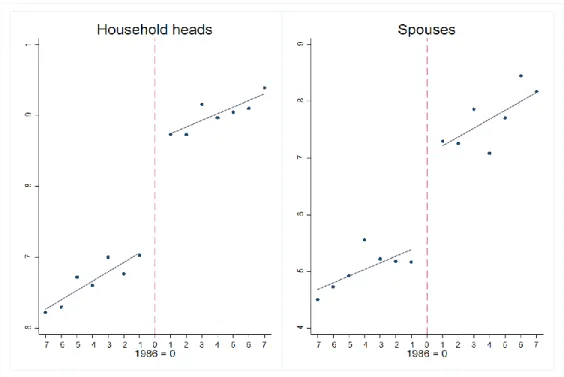
Our findings suggest that there has been an increase in junior high school completion rates for both household heads and their spouses as a result of the 1997 compulsory schooling law change: completion rate increased by around 11 and 16 percentage points, respectively, as shown in Figure 1. Using our measures of financial behavior, we find that there is little effect of education on household debt incurrence, and consequently on its respective forms. We find a similar result for our saving behavior measures as well, with the exception of bank savings: we show that a 5.3 percentage point increase in household savings held through a financial intermediary can be attributed to the treatment status of the household head, and as such to his/her level of education. The main form in which these savings are held seems to be that of bank accounts: we see an increase of 4.5 ppts in

(15)

4

Figure 1: Proportion of individuals with at least junior high school degree by birth cohort.

the propensity to have a bank account for the whole sample, while the same estimates for other, more sophisticated instruments are small and insignificant. The results seem to be fully driven by the effect of the reform on financial behavior on the unmarried sample, where the estimates are significant and around 13 ppts. There seems to be no effect of education on household debt or saving decisions for the married sample.

1.2 Related literature

Our work contributes to the limited but growing literature that analyses the relationship between education and financial market participation of households. Cole, Paulson and Shastry’s (2014) work is one of the first that uses exogenous variation generated by changes in compulsory schooling legislation to establish a causal relationship between education and financial market participation. While one can argue that their econometric specification does not entirely bypass the endogeneity issue (namely, their inclusion of an income polynomial), it serves to highlight the issue of financial illiteracy, and its effect

(16)

5

on financial market participation. This aspect of the analysis has been studied

extensively: Cole, Paulson and Shastry (2016) find that traditional, high school-level financial and mathematics education does not encourage financial participation. Other studies have found that financially illiterate individuals tend to have little to no retirement plans, borrow more and hold fewer financial assets (Lusardi & Mitchell, 2007; Lusardi & Tufano, 2015). We add to this literature by attempting to analyze this question in the context of a developing country – Turkey – which has a shallow, but quickly developing financial market. Our work is closely related in spirit to those of Garsia and Tessada (2013) and Park and Son (2015), who define educational attainment as high school and college completion, respectively. Garcia and Tessada (2013) relate the education of the household head to higher propensities of financial market participation, while Park and Son (2015) find that the educational attainment of the household head positively impacts the household’s propensity to hold any savings, and their amount.

This study also relates to the extensive literature that uses changes in compulsory schooling laws to determine the impact of education in employment and earnings (Angrist & Krueger, 1991; Harmon & Walker, 1995; Oreopoulos, 2006), health, happiness and social standing (Oreopoulos, 2007; Oreopoulos & Salvanes, 2011;

Kemptner, Jürges & Reinhold, 2011; Clark & Royer, 2013), fertility (Black, Devereux & Salvanes, 2008; Cygan-Rehm & Maeder, 2013), cognitive ability (Crespo, Lòpez-Noval & Mira, 2014), criminal activity (Machin, Olivier & Vujić, 2011) and other outcomes. Moreover, previous studies have used the same reform to establish the impact of increases in education on several outcomes of interest in Turkey, including, but not limited to labor market outcomes (Mocan, 2014; Aydemir & Kırdar, 2017; Torun, 2018), religiosity (Güleşçi & Meyersson, 2014; Cesur & Mocan, 2018), health and happiness (Dursun & Cesur, 2016; Dursun, Cesur & Kelly, 2017; Dursun, Cesur & Mocan, 2018); fertility and gender equality (Dinçer, Kaushal & Grossman, 2014; Kırdar, Dayıoğlu & Koç, 2018; Güleşçi, Meyersson & Trommlerova, 2019), prosocial behavior (Akar, Akyol & Okten, 2019).

(17)

6

1.3 The 1997 Reform

Prior to the 1997 reform, compulsory schooling in Turkey consisted of only 5 years of primary education. After its completion, students could choose to either drop out, or continue their education in either general, vocational or religious schools. The Basic Education Law passed in 1997 required that, starting from the 1998-1999 academic year, all children who completed the fifth grade continue to the eighth. This policy was not meant to be retroactive, however it was expected that many students in the basic education age, who had already dropped out, would return to school. To facilitate the attendance of this particular subgroup, the government implemented distance learning methods in an open education program (Dülger, 2004).

While the government supported the program as a way of decreasing poverty and social disparity, a central motivation behind the policy change was to curb religious education in the country (Aydemir & Kırdar, 2017). The Islamist party had won the parliamentary majority in 1995 and secular groups, mainly in the military and judiciary, introduced a new set of laws to prevent the expansion of Islamist influence. The extension of compulsory schooling was included in the new legislation. In addition, vocational and religious schools at the secondary level were closed and the traditional diploma rewarded at the end of the fifth year was abolished. Extensive, country-wide funding was provided for the expansion of the education system in both infrastructure and staffing, in order to handle the expected increase in active students. This intervention was also independent of the macroeconomics of Turkey at the time; thus, it did not coincide with other policies that would have an effect on schooling outcomes (Aydemir & Kırdar, 2017).

The Basic Education program had a significant impact on the student population in Turkey. As a result of the reform and the incentives created to promote compliance, enrollment in grades one through eight increased with over 1.1 million students, raising the primary school enrollment rate from 85.63% in 1997 to 96.30% in 2002. The increase in enrollment rates was higher for females that for males, with the enrollment of females in rural areas experiencing an increase of 162% in the first year alone (Dülger, 2004).

(18)

7

CHAPTER 2 EMPIRICAL STRATEGY

2.1 Data and variables

We use data from the 2016 Family Structure Survey, conducted by the Turkish Statistical Institute jointly with the Ministry of Family and Social Policies. The sample contains responses from 17,239 households and 35,475 individuals aged 15 and older on a variety of questions intended to determine individuals’ lifestyle and family structure, including their background information, labor market position, welfare, financial behavior and marital status. The survey was conducted on a household basis, with members of the household selected randomly and interviewed privately.

In the individual response part of the survey, individuals are asked questions regarding their financial decisions. Specifically, they are asked if i) they have any interest income and ii) any real estate income that they have personally earned in the last year.

Correspondingly, in the household questionnaire, one individual from each household is asked if the household has any savings or debt, and if the answer is ‘YES’, polar

questions are asked to extract the details. With relation to financial market participation, the household representative is asked whether the household has received any bank loans or is under credit card debt, or if household savings are i) kept in a bank account, ii)

(19)

8

stocks, iii) bonds or iv) fund certificate. Using these responses, we define our outcome variables as dummies that take 1 if the respondent admits to owning/owing the specific asset/liability, and 0 otherwise. Detailed explanations for each variable are included in Table 16 in the Appendix.

Table 1 reports the descriptive statistics of the household heads and their spouses. The treatment status is defined as exposure to the 1997 reform, and is determined by the year of birth. The reform did not affect those who were 12 years old or older in 1997, as they would have finished five years of schooling and were not required to return, so these individuals – born in 1985 or earlier – will constitute the control group. Those who were 10 years old or younger in 1997 were undoubtedly affected by the reform, so the cohort of those born in 1987 or later will be included in the treatment group. The treatment status of those born in 1986 (11 years old in 1997), however, is uncertain as it depends on their birth month and their school starting year. Thus, we exclude this cohort in our baseline estimations.

In Panel A of Table 1 we present descriptive statics for the educational outcomes of household heads and their spouses, by the treatment status of the household head. 74.4% of the household heads in the sample have completed at least junior–high, which entails eight years of schooling. The proportion is larger for the treated sample, which has been exposed to the change in education laws: 90.4% of treated household heads have received their junior-high diploma, compared to 67.5% in the untreated group. The same statistics are comparatively lower for the spouses’ subsample, however, the difference in

educational attainment between treatment and control groups can still be observed: while 81.9% of spouses of the household heads in the treatment group have received at least eight years of schooling, only 62.4% of the untreated spouses have done so.

Panels B and C of Table 1 report the statistics for households’ financial market behavior, by the treatment status of the household responsible. Households with treated (and presumably more educated) responsibles seem to be indebted slightly less, but engage more with the financial market when it comes to saving. However, overall, there seems to be little difference between the treatment and control groups for most measures of

(20)

9

Table 1: Descriptive statistics (by treatment status)

Heads Spouses

All Treatment Control All Treatment Control

(1) (2) (3) (4) (5) (6)

Mean Mean Mean Mean Mean Mean

Sd. Sd. Sd. Sd. Sd. Sd.

A - Educational outcomes

Junior high school 0.744 0.904 0.675 0.651 0.819 0.624 (0.444) (0.300) (0.469) (0.457) (0.385) (0.485) High school 0.557 0.643 0.542 0.437 0.483 0.439 (0.495) (0.480) (0.498) (0.496) (0.500) (0.496) College 0.323 0.372 0.302 0.230 0.258 0.244 (0.468) (0.484) (0.459) (0.421) (0.438) (0.430) B - Debt Any debt 0.374 0.362 0.378 (0.484) (0.481) (0.485) Bank loan 0.331 0.305 0.328 (0.470) (0.461) (0.470) Credit card debt 0.096 0.090 0.098

(0.294) (0.286) (0.297) C - Saving Any saving 0.168 0.180 0.162 (0.374) (0.384) (0.369) Bank saving 0.091 0.107 0.084 (0.287) (0.309) (0.277) Bank account 0.089 0.103 0.082 (0.284) (0.304) (0.275) Other 0.003 0.003 0.003 (0.055) (0.058) (0.053) D - Labor market outcomes

Employed 0.820 0.791 0.832 0.347 0.311 0.358 (0.384) (0.407) (0.374) (0.475) (0.463) (0.480) Wage earner 0.653 0.660 0.652 0.294 0.282 0.298 (0.476) (0.475) (0.477) (0.455) (0.451) (0.458) Private sector 0.631 0.583 0.651 0.244 0.232 0.249 (0.483) (0.493) (0.477) (0.430) (0.422) (0.433) E - Individual characteristics Age 31.65 26.34 33.93 30.16 25.83 31.62 (4.014) (1.955) (2.025) (5.232) (4.143) (4.731) Sex 0.801 0.758 0.820 0.133 0.173 0.120 (0.399) (0.429) (0.385) (0.340) (0.378) (0.325) Married 0.816 0.686 0.890 (0.387) (0.464) (0.313) Observations 3003 901 2102 2392 602 1790

(21)

10

the control. It is of note, however that in all related measures, it seems that a higher portion of Turkish households admits to being indebted compared to owning any financial asset, irrespective of the treatment status of their household head. In Panel D, we show the summary statistics for the labor market outcomes of the

individuals in our sample: notice that there is a large difference between household heads and their spouses in both employment status and having wage income (only 34.7% of spouses are employed versus 82.0% of household heads). This is in line with Turkey’s long-term female labor force participation rate, which has remained at a low 32%, and as we see in Panel E, more than 80% of the sample of the household heads is male,

compared to only about 13% of the spouses. In addition, Panel E of Table 1 provides a brief overview of the marriage market outcomes of the individuals in our sample and their ages. It is of note that most of the sample is in a cohabiting relationship (81.6% is ‘married’), where the rates are higher for the untreated sample (89.0% to 68.6%). This could be also related to the significantly lower average age of the individuals in the treated cohort, which decreases their propensity to being married or in a serious relationship.

2.2 Identification

The 1997 education reform provides an opportunity to investigate the relationship between education and household financial behavior by comparing the outcomes of the cohorts that are included in the treatment group, to those born too early to be affected by the policy change. The 1997 Basic Education reform was an unexpected change in compulsory schooling laws that only affected the years of schooling of the impacted cohort, and had no impact on other related variables, as it did not initiate a change in the programs or the courses taught in schools (Dülger, 2004). Therefore, the 1997 law change is widely accepted to have impacted the educational attainment of the relevant population exogenously and this reform is used in the literature to account for the endogeneity of education when analyzing its causal impact on many outcomes of interest through the Instrumental Variables (IV) technique.

(22)

11

For our purposes, while the instrument for education – constructed based on the treatment status of the individual – can be considered exogenous to household’s financial decision making, it fails to satisfy the exclusion restriction assumption required to implement the IV method. The reason stems from the fact that the policy change was implemented universally, with little gender or status discrimination: the only variable that determines whether an individual was affected by the reform is their year of birth. Thus, when trying to analyze the effect of education on household-level outcomes, we need to account for the fact that, given assortative mating, members of the same couple are highly probable to share the same treatment status. Since household financial decisions are assumed to be made jointly, this creates a second channel though which education may affect household financial behavior. Hence, it is not possible for us to successfully establish a causal relationship between education and financial market participation, given the data at hand. What we do instead, is use this reform in measuring the impact of a change in

compulsory schooling laws on household financial decisions.

We first run regressions to check if the reform had an impact on the household head having received at least junior high school degree, and then do the same for their spouse. This will be our empirical test on whether the use of the IV method is appropriate in this case. We use birth year as our running variable, due to one’s inability to control it. Among the individuals born close to our cutoff of 1986, being born after this year and thus having a higher probability of being affected by the exogenously applied change in schooling laws cannot be manipulated by the individual under observation, making this a randomly assigned treatment. The estimates are derived using Equation 1:

Educationi = β0 + β1 Reformi + β2 Xi + νi, (1) where our dependent variable Educationi is an indicator for the individual i having at least received a junior-high diploma. Reformi is a dummy that takes 1 if the individual i has been affected by the change in schooling laws, which corresponds to them having been born after 1986. Xi is the vector of control variables, which include a dummy variable for the individual being male, having spent the formative years in a rural area, childhood region and residence fixed effects, and the interactions between the trend

(23)

12

dummies and the gender of individual i (note that i refers to the head of the respective household or their spouse in separate specifications).

Having tested – and subsequently denied – the validity of Reform as an instrument for

Education, we estimate RF regressions for our outcomes of interest as follows:

Household financial behaviorj = ρ0 + ρ1 Reformij + ρ2 Xj + ηj. (2) where Household financial behaviorj is one of the 7 measures of financial behavior that we have defined for household j, and Reformij is a dummy variable that takes 1 if the responsible i of household j has been affected by the 1997 change in education policy. It is important to clarify what our empirical strategy identifies. The coefficient ρ1 represents the effect of the reform on household financial behavior outcomes, which is the policy-related impact of compulsory schooling laws. However, as we will show later, there is a strong positive relationship between the variable that indicates compulsory schooling – our treatment variable Reformij – and the educational outcomes of the household heads in our sample. Thus, while we cannot attach a causal interpretation to these estimates, this method does allow us to confidently make inferences on the nature of the relationship between education and household financial decisions. In addition, capturing the impact of this compulsory schooling reform on financial outcomes is of interest in and of itself. The reform of 1996 had a larger impact on the educational

outcomes of particularly disadvantaged groups, so any income-relevant externality of this policy is of value to the policy maker.

(24)

13

CHAPTER 3 MAIN RESULTS

3.1 Schooling outcomes

To examine the effect of education on household financial behavior outcomes through the exogenous variation generated by the change in education policy, it is common to first look into the impact of this reform on schooling outcomes. Table 2 reports the schooling effect of the reform, defined as having completed at least junior high school (i.e. received eight years of schooling), high school or college, for household heads and their spouses. These different definitions of education are important not only in determining the extent of the effect of the reform, but also in interpreting the effect of knowledge on financial market participation. The estimates report the effect of the reform on junior high school completion (Equation 1), where we construct a dummy variable that takes one if the individual has been affected by the reform. We control for childhood region and current residence fixed effects, the sex of the household head, whether they have spent their first 15 years in a rural residence, the trends in treatment assignment and their interactions with the sex of the household head.

(25)

14

Table 2: Effect of Reform on education

Education level

(1) (2) (3)

Junior high school High school College

A - Household heads Reform 0.1136*** 0.0812** 0.0018 (0.033) (0.038) (0.041) F-Stat 12.414 4.606 0.002 Observations 3003 3003 3003 B - Spouses Reform-spouse 0.1554*** 0.0556 0.0186 (0.040) (0.037) (0.037) F-Stat 15.219 2.272 0.261 Observations 2179 2179 2179

Notes: Columns (1), (2) and (3) report the effect of the treatment in educational attainment. The sample consists of individuals born between 1979 and 1993, with ages ranging from 22 to 37 years old. The dependent variables are Junior high school, High school and College, which are dummies that take 1 if the individual has received at least a junior high school diploma, which corresponds to having completed at least 8 years of schooling, or a high school or college diploma, respectively. Reform and Reform-spouse are dummy variables that take 1 if the household head or their spouse belongs to the treatment group, i.e. was born after 1986, respectively. The 1986 cohort is not included. The control variables include a dummy for having spent the first 15 years in a village, childhood and current residence fixed effects, control and treatment time trends and their interaction with the sex of the individual. The selected bandwidth is 7 (by the CCT algorithm). Standard errors are clustered at region-of-birth-by-birth-year level.

*, **, *** denote significance levels of 10%, 5% and 1%, respectively. Standard errors are in parentheses.

Source: 2016 Family Structure Survey

The results reported in Table 2 suggest that the reform has a significant impact on junior high-school completion for all individuals in the sample: the propensity of having at least a junior-high diploma increased by 11.36 ppts for household heads and 15.54 ppts for their spouses, with the later predictively having been more affected due to their higher concentration of females. These results are consistent with what is usually found in the literature. Also consistent with the literature, the reform seems to be a weak instrument with regards to high school and college completion for either subsample. As a result, the definition of education that we will be using going forward is having received at least a junior high school diploma, which implies the individual has received at least eight years

(26)

15

Table 3: Effect of Reform on spouses’ education

Education level of spouses

(1) (2) (3)

Reform-spouse Junior high school High school

Reform _0.12*** _0.031 _0.053

(0.033) (0.037) (0.041)

Observations ₂₂₁₄ ₂₃₉₂ ₂₃₉₂

Notes: Columns (1), (2) and (3) report the effect of the treatment status of the household head in the treatment status and educational attainment of their spouse. The sample consists of individuals born between 1979 and 1993, with ages ranging from 22 to 37 years old. The dependent variables are Reform-spouse, Junior high

school and High school, measured by dummies that take 1 if the spouse has been impacted by the reform and

has received at least a junior-high or a high school diploma, respectively. Reform and Reform-spouse are dummy variables that take 1 if the household head or their spouse belongs to the treatment group, i.e. was born after 1986, respectively. The 1986 cohort is not included. The control variables include a dummy for having spent the first 15 years in a village, childhood and current residence fixed effects, control and treatment time trends and their interaction with the sex of the household head. The selected bandwidth is 7 (by the CCT algorithm). Standard errors are clustered at region-of-birth-by-birth-year level.

of general education. However, it is of note that this reform has impacted both the household heads and their spouses, hinting at the existence of two separate channels through which the same reform may impact our financial market outcomes. To test this, we run regressions to check the relationship between the treatment status of the

household head and that of their spouse, the results of which are presented in Table 3. In here, we can see that there exists a strong and very significant relationship between the treatment status of the household head and that of their spouse. These results confirm our suspicion that the variable ‘Reform’ does not satisfy the exclusion restriction. Hence, it is not a valid instrument for the educational attainment of the household head in this case, thus ruling out the use of IV as an estimation strategy.

3.2 Financial behavior outcomes

Having ruled out the possibility of establishing a causal relationship between education and household financial behavior, we turn our attention to the impact of the reform itself.

(27)

16

Table 4: Effect of junior high school completion on household financial behavior

(1) (2) (3) (4) (5) (6) (7)

Any debt Bank debt Bank loan Credit card debt Any saving Bank saving Bank account

A - Whole sample

Junior high school 0.082*** 0.10*** 0.11*** 0.045*** 0.14*** 0.072*** 0.070***

(0.020) (0.019) (0.019) (0.013) (0.014) (0.0098) (0.0097)

Observations 3003 3003 3003 3003 3003 3003 3003

B - Married sample

Junior high school 0.084*** 0.11*** 0.11*** 0.040*** 0.13*** 0.059*** 0.057***

(0.022) (0.021) (0.020) (0.015) (0.014) (0.0100) (0.0099)

Observations 2451 2451 2451 2451 2451 2451 2451

C - Unmarried sample

Junior high school 0.11 0.11* 0.10* 0.076** 0.19*** 0.14*** 0.14***

(0.064) (0.056) (0.055) (0.029) (0.030) (0.033) (0.035)

Observations 552 552 552 552 552 552 552

Notes: Columns (1), (2), (3) and (4) report the Ordinary Least Squares results for the measures of debt, columns (5), (6) and (7) report the same results for the saving measures. The sample consists of individuals born between 1979 and 1993, with ages ranging from 22 to 37 years old. The treatment group consists of individuals born after 1986, the control group consists of individuals born before 1986. The 1986 cohort is not included. Any debt is an indicator variable for the household having any borrowings of any form. Bank debt is an indicator for household borrowing being recorded in a bank. Bank loan and Credit card debt are dummies that take 1 for the respective form of debt. Any saving is an indicator variable for the household having saving in any format. Bank saving in an indicator for household saving being recorded in a bank. Bank account is a dummy that takes 1 if savings are kept in a bank account. Junior high school is a dummy variable that takes 1 if the household head has received at least a junior-high school diploma, corresponding to 8 years of education. The control variables include a dummy for having spent the first 15 years in a village, childhood and current residence fixed effects, control and treatment time trends and their interaction with the sex of the household head. The selected bandwidth is 7 (by the CCT algorithm). Standard errors are clustered at region-of-birth-by-birth-year level for the whole and married sample, and by birth year for the unmarried sample.

(28)

17

First, however, we run simple OLS regressions of our outcomes on junior high school completion and the other control variables, to get a sense of the overall relationship. Table 4 presents the estimates both for the whole sample of household responsibles and the married and single subsamples. There seems to be a strong positive relationship between the household head’s junior high school completion and the household’s

participation in the financial market, both as a borrower and as a saver. We notice that the household head having received at least eight years of schooling is significantly

positively correlated to the household having received a bank loan, but also having any savings of any form. The estimates are positive and significant for all the more specific definitions of financial market participation, in all of the three presented subsamples. Panel A of Table 5 reports the results of the RF estimation (Equation 2) for each of our measures of household debt and saving. Relying on its recognized exogeneity and using the reform to determine the treatment status of the household head, Table 5 shows a lack of impact of the reform and the household’s propensity to borrow, for all of our debt measures. The household head having been impacted by the 1997 reform increases the household’s propensity to hold savings in a bank by a significant 5.3 ppts. This is further broken down into whether savings are held in an account or not. We notice that the reform increases the propensity of having a bank account by 4.5 ppts.

However, these are the results estimated for the whole sample, where we have household heads in different marriage market positions. To bypass the confounding effect of the spouse’s treatment status, we split the sample into two: married and unmarried. The results for the married sample are reported in Panel B, and there seems to be no

significant association between the treatment status of the household head and household financial market behavior. Interestingly, when looking at the same results for the

unmarried sample in Panel C, we retrieve estimates similar in nature to those of the whole sample: the impact of the reform is insignificant across the board, with the exception of bank savings, where we do see a 13 ppts increase, and again, they are almost fully kept as accounts. This makes us believe that the results we retrieved in Panel A are fully driven by the significantly positive relationship between the treatment status of the household head and the propensity to hold a bank account in this particular subsample.

(29)

18

Table 5: Effect of Reform on household financial behavior

(1) (2) (3) (4) (5) (6) (7)

A - Whole sample Reform 0.046 0.020 0.012 0.028 0.034 0.053** 0.045* (0.040) (0.039) (0.037) (0.028) (0.033) (0.024) (0.024) Observations 3003 3003 3003 3003 3003 3003 3003 B - Married sample Reform 0.065 0.047 0.036 0.028 0.036 0.039 0.031 (0.045) (0.045) (0.042) (0.032) (0.035) (0.027) (0.025) Observations 2451 2451 2451 2451 2451 2451 2451 C - Unmarried sample Reform -0.066 -0.082 -0.078 -0.0026 0.033 0.13*** 0.13** (0.070) (0.073) (0.063) (0.081) (0.063) (0.044) (0.048) Observations 552 552 552 552 552 552 552

Notes: Columns (1), (2), (3) and (4) report the Reduced Form results for the measures of debt, columns (5), (6) and (7) report the same results for the saving measures. The sample consists of individuals born between 1979 and 1993, with ages ranging from 22 to 37 years old. The treatment group consists of individuals born after 1986, the control group consists of individuals born before 1986. The 1986 cohort is not included. Any debt is an indicator variable for the household having any borrowings of any form. Bank debt is an indicator for household borrowing being recorded in a bank. Bank loan and Credit card debt are dummies that take 1 for the respective form of debt. Any saving is an indicator variable for the household having saving in any format. Bank saving in an indicator for household saving being recorded in a bank. Bank account is a dummy that takes 1 if savings are kept in a bank account. Reform is a dummy variable that takes 1 if the household head has been impacted by the reform i.e. has been born after 1986. The control variables include a dummy for having spent the first 15 years in a village, childhood and current residence fixed effects, control and treatment time trends and their interaction with the sex of the household head. The selected bandwidth is 7 (by the CCT algorithm). Standard errors are clustered at region-of-birth-by-birth-year level for the whole and married sample, and by birth year for the unmarried sample.

(30)

19

CHAPTER 4 ROBUSTNESS

4.1 Robustness checks

In this section, we present some of the tests we conducted to ascertain the validity of our results.

We begin by re-estimating our model of interest (Equation 2) with different bandwidths, in order to rule out the possibility that our estimates emerge serendipitously for this specific sample. The results are presented in Table 6, and we can see that they are similar to those in Table 5, both in significance – or lack thereof – and in magnitude. There seems to be no impact of the treatment on any of the debt measures irrespective of the selected bandwidth (note that the bandwidth used for our main analysis is 7). Having any bank savings (and, consequently, having an account) starts to be impacted by the reform at higher bandwidths, mainly due to the increased inclusion of the control group, that is older on average, but the magnitude of the effect does not vary too much.

(31)

20

Table 6: Robustness check: bandwidth selection

Selected bandwidth around 1986

(1) (2) (3) (4) (5) (6) (7) 4 5 6 7 8 9 10 Any debt 0.084 0.042 0.055 0.046 0.046 0.049 0.041 (0.058) (0.051) (0.045) (0.040) (0.038) (0.036) (0.035) Bank debt 0.067 0.030 0.033 0.020 0.034 0.038 0.035 (0.055) (0.049) (0.043) (0.039) (0.037) (0.035) (0.033) Bank loan 0.038 0.014 0.018 0.012 0.023 0.024 0.021 (0.052) (0.046) (0.041) (0.037) (0.035) (0.033) (0.032) Credit card debt 0.069* 0.040 0.040 0.028 0.026 0.027 0.026

(0.038) (0.034) (0.030) (0.028) (0.026) (0.025) (0.024) Any saving 0.0064 0.0026 0.032 0.034 0.031 0.027 0.028 (0.047) (0.042) (0.037) (0.033) (0.031) (0.030) (0.029) Bank saving 0.037 0.026 0.047* 0.053** 0.051** 0.052** 0.052** (0.035) (0.033) (0.028) (0.024) (0.023) (0.022) (0.022) Bank account 0.022 0.012 0.037 0.045* 0.043* 0.045** 0.044** (0.033) (0.031) (0.027) (0.024) (0.022) (0.021) (0.021) Observations 1761 2167 2580 3003 3402 3773 4118

Notes: The table reports the Reduced Form results for all our borrowing and saving measures under different bandwidths around the cutoff of 1986. The sample consists of individuals born between 1979 and 1993, with ages ranging from 22 to 37 years old. The treatment group consists of individuals born after 1986, the control group consists of individuals born before 1986. The 1986 cohort is not included. Any debt is an indicator variable for the household having any borrowings of any form. Bank debt is an indicator for household borrowing being recorded in a bank. Bank loan and Credit card debt are dummies that take 1 for the respective form of debt. Any saving is an indicator variable for the household having saving in any format.

Bank saving in an indicator for household saving being recorded in a bank. Bank account is a dummy that

takes 1 if savings are kept in a bank account. The treatment variable – Reform – is a dummy variable that takes 1 if the household head has been impacted by the reform i.e. has been born after 1986. The control variables include a dummy for having spent the first 15 years in a village, childhood and current residence fixed effects, control and treatment time trends and their interaction with the sex of the household head. Standard errors are clustered at region-of-birth-by-birth-year level.

Another point on contention could be the fact that due to the uncertainty of their

treatment status, our main estimation strategy does not take into consideration household heads born in 1986. In doing so, we implicitly assume that omitting this cohort does not impact our results. To test this claim, we re-run Equation 2 by including the 1986 cohort. The treatment status of these individuals is still unknown, but since the variable ‘Reform’ is a dummy that takes either 0 or 1, we set this variable equal to 0.5 for this cohort. The results in Table 7 are consistent with our earlier results.

(32)

21

Table 7: Robustness check: keeping the 1986 cohort

(1) (2) (3) (4) (5) (6) (7)

A - Whole sample Reform 0.048 0.020 0.013 0.024 0.031 0.052** 0.044* (0.039) (0.038) (0.036) (0.027) (0.032) (0.024) (0.023) Observations 3216 3216 3216 3216 3216 3216 3216 B - Married sample Reform 0.067 0.045 0.035 0.022 0.034 0.036 0.029 (0.044) (0.043) (0.041) (0.031) (0.034) (0.026) (0.025) Observations 2621 2621 2621 2621 2621 2621 2621 C - Unmarried sample Reform -0.054 -0.073 -0.067 0.0042 0.020 0.12** 0.12** (0.066) (0.071) (0.063) (0.085) (0.074) (0.047) (0.053) Observations 595 595 595 595 595 595 595

Notes: Columns (1), (2), (3) and (4) report the Reduced Form results for the measures of debt, columns (5), (6) and (7) report the same results for the saving measures. The sample consists of individuals born between 1979 and 1993, with ages ranging from 22 to 37 years old. The treatment group consists of individuals born after 1986, the control group consists of individuals born before 1986. The 1986 cohort is included. Any debt is an indicator variable for the household having any borrowings of any form. Bank debt is an indicator for household borrowing being recorded in a bank. Bank loan and Credit card debt are dummies that take 1 for the respective form of debt. Any saving is an indicator variable for the household having saving in any format. Bank saving in an indicator for household saving being recorded in a bank. Bank account is a dummy that takes 1 if savings are kept in a bank account. Reform is a dummy variable that takes 1 if the household head has been impacted by the reform i.e. has been born after 1986. The control variables include a dummy for having spent the first 15 years in a village, childhood and current residence fixed effects, control and treatment time trends and their interaction with the sex of the household head. The selected bandwidth is 7 (by the CCT algorithm). Standard errors are clustered at region-of-birth-by-birth-year level for the whole and married sample, and by birth year for the unmarried sample. *, **, *** denote significance levels of 10%, 5% and 1%, respectively.

Standard errors are in parentheses. Source: 2016 Family Structure Survey

(33)

22

4.2 Placebo tests

As a final check for the robustness of our results, we construct placebo tests around different birth years. The purpose of this is to eliminate any possibility of the existence of a systematic relationship between the birth year of the household head and the financial market participation outcomes or educational attainment that could be driving the results. The test is conducted by gradually shifting the cutoff year away from 1986 in either direction and redefining the treatment variable accordingly. These results are shown in Tables 8 and 9. The preliminary results in Figure 3 (see Appendix) show that, under these hypothetical reforms, there is little discontinuity in junior high school completion for the household heads in our sample the more we push the cutoff year away from 1986. The estimates in Table 8 show that the placebo reform does not have a significant positive effect on schooling for household heads. This confirms that our results are not driven by any random trend between junior high school completion and the birth years of the individuals in our sample.

Table 8: Effect of placebo Reform on education

Junior high school completion

(1) (2) (3) (4) (5) (6) (7)

1983 1984 1985 1987 1988 1989 1990

Reform -0.0097 0.017 0.084*** 0.092*** 0.075** 0.026 0.0051

(0.030) (0.030) (0.032) (0.033) (0.034) (0.040) (0.042)

Observations 3716 3493 3248 2710 2451 2146 1878

Notes: The table shows the impact of the placebo treatment on the educational attainment of household heads. The dependent variable is Junior high school, measured by a dummy that take 1 if the individual has received at least a junior-high diploma, which corresponds to having completed at least 8 years of schooling. The treatment variable – Reform – is a dummy variable that take 1 if the household head belongs to the treatment group. The control variables include a dummy for having spent the first 15 years in a village, childhood and current residence fixed effects, control and treatment time trends and their interaction with the sex of the individual. The cohort belonging to each cutoff is not included. The selected bandwidth is 7 (by the CCT algorithm). Standard errors are clustered at region-of-birth-by-birth-year level.

(34)

23

We take a similar approach to confirming the validity of our Reduced Form results. The estimates presented in Table 9 suggest that there is no significant effect of the

hypothetical reforms on our outcome variables. This serves to confirm that the

relationship that we capture is one between the treatment status of the household head (‘treatment’ here refers to having been impacted by the 1986 Basic Education Reform) and our measures of household financial market participation, and cannot be attributed to pre-existing trends.

Table 9: Effect of placebo Reform on household financial behavior

Placebo cutoff (1) (2) (3) (4) (5) (6) (7) 1983 1984 1985 1987 1988 1989 1990 Any debt 0.026 0.00058 0.050 -0.0066 -0.050 -0.035 -0.017 (0.034) (0.038) (0.035) (0.045) (0.046) (0.051) (0.055) Band debt 0.038 -0.0027 0.026 0.0061 -0.033 -0.023 0.0065 (0.032) (0.037) (0.035) (0.045) (0.044) (0.045) (0.051) Bank loan 0.031 -0.015 0.014 0.011 -0.0097 -0.00068 0.014 (0.032) (0.036) (0.034) (0.045) (0.044) (0.045) (0.051) Credit card -0.0043 -0.018 -0.00062 0.0068 -0.027 -0.018 -0.020 (0.019) (0.023) (0.023) (0.029) (0.027) (0.031) (0.032) Any saving 0.039 0.014 0.017 0.033 0.017 -0.058 -0.014 (0.027) (0.030) (0.031) (0.034) (0.037) (0.038) (0.047) Bank saving 0.015 0.011 0.046* 0.022 0.014 -0.028 -0.017 (0.021) (0.023) (0.024) (0.026) (0.028) (0.035) (0.044) Bank account 0.013 0.0055 0.037 0.025 0.024 -0.019 -0.011 (0.021) (0.023) (0.023) (0.026) (0.028) (0.034) (0.044) Observations 3716 3493 3248 2710 2451 2146 1878

Notes: The table shows the Reduced Form estimates of the impact of the placebo Reform on our household financial behavior measures. Any debt is an indicator variable for the household having any borrowings of any form. Bank debt is an indicator for household borrowing being recorded in a bank. Bank loan and Credit

card debt are dummies that take 1 for the respective form of debt. Any saving is an indicator variable for the

household having saving in any format. Bank saving in an indicator for household saving being recorded in a bank. Bank account is a dummy that takes 1 if savings are kept in a bank account. Reform is a dummy variable that takes 1 if the household head has been impacted by the reform i.e. has been born after 1986. The control variables include a dummy for having spent the first 15 years in a village, childhood and current residence fixed effects, control and treatment time trends and their interaction with the sex of the household head. The cohort belonging to each cutoff is not included. The selected bandwidth is 7 (by the CCT algorithm). Standard errors are clustered at region-of-birth-by-birth-year level.

(35)

24

CHAPTER 5 CONCLUDING REMARKS

The current literature on financial market participation exploits the wealth of data observed in high income countries to determine the correlative or causal relationships between education and individual or household financial decision making. The aim of this paper is to investigate the effects of schooling on household financial behavior in a developing country – Turkey. We define our level of education as having completed at least junior high-school, and use the exogenous variation provided by a change in

compulsory schooling laws to model the relationship between the educational attainment of the household head and household financial market participation, with respect to several measures of borrowing and saving.

Our results suggest that the 1997 change in educational policy increased junior high school completion rates of Turkish household heads by 11 ppts, and with a higher impact being observed in their spouses (almost 16 ppts increase). We find that there is no effect of this legislative change on household borrowing decisions, but the household head having been impacted by the reform is associated with an increase of 5.3 ppts in the propensity to hold savings in a financial institution. Due to the insignificance of the other saving measures, we conclude that this result is mainly driven by the effect of the reform

(36)

25

on the propensity to hold an interest paying bank account, which we report to increase by 4.5 ppts. These results are robust to a series of robustness tests.

It would make for an interesting exercise to look into the reasons behind the weak impact of compulsory schooling on household financial behavior in Turkey. One explanation can be found in the literature: one needs advanced mathematical and financial training to be able or willing to navigate the financial market (Cole et. al., 2016). There is anecdotal evidence that this is not the case for Turkey – students receive only basic mathematical and almost no economic or financial training throughout their entire general education, and for some, this persists into their high education. This could contribute to wide-spread financial illiteracy, which in turn discourages participation in the financial market. If that is the case, the positive impact of compulsory schooling on bank saving that we observe here could be explained by the development of the financial market itself: the reform enhances educational attainment and thus leads to higher paying jobs, which, in time, have started to supply wages through bank transfers, providing an easy access to the financial market for most Turkish white-collar employees.

Some final remarks are in order. First, there are important distinctions between our treatment and control groups, which cannot be entirely attributed to their treatment status. Namely, individuals in the treatment group are, on average, much younger than those in the control group (by almost 7 years), and their ‘married’ proportion is much lower (68.6% versus 89.0%). This is an issue of timing, both in the application of the 1997 reform and the collection of our data. Thus, at least part of the reason as to why we see such a small impact of this policy in financial market participation can be credited to these differences. Secondly, our methodology allows us to measure the impact of the compulsory schooling policy, and while we believe it to be tightly related to the

educational attainment of the individuals in our sample, the estimates we present are not a precise measure of the relationship between education and household financial market participation. Finally, it is worth noting that our estimates are driven by a change in middle schooling, thus they do not rule out the possibility of significant returns to schooling at higher levels.

(37)

26

BIBLIOGRAPHY

Abadie, A., Athey, S., Imbens, G. W., & Wooldridge, J. (2017). When Should You Adjust Standard Errors for Clustering? NBER Working paper. doi: 10.3386/w24003 Acemoglu, D., & Angrist, J. (2000). How large are Human-Capital Externalities?

Evidence from Compulsory Schooling Laws. NBER Macroeconomics Annual, 15(2000), 9–59. doi: 10.2307/3585383

Agarwal, S., & Mazumder, B. (2013). Cognitive Abilities and Household Financial Decision Making. American Economic Journal: Applied Economics, 5(1): 193–207. doi: 10.1257/app.5.1.193

Akar, B., Akyol, P., & Okten, Ç. (2019). Education and Prosocial Behavior: Evidence from Time Use Survey. IZA Discussion Paper, 12558. Retrieved from

https://ssrn.com/abstract=3445824

Angrist, J.D., & Krueger, A. B. (1991). Does compulsory school attendance affect schooling and earnings. Quarterly Journal of Economics, 106(4), 979–1014. doi: 10.2307/2937954

Angrist, J.D., & Krueger, A. B. (1999). Empirical strategies in labor economics.

Handbook of Social Economics, Vol. 3A, 1277-1366.

Aydemir, A., & Kırdar, M. (2017). Low Wage Returns to Schooling in a Developing Country: Evidence from a Major Policy Reform in Turkey. Oxford Bulletin of

Economics and Statistics, 79, 6(2017), 0305–9049. doi: 10.1111/obes.12174

Black, S. E., Devereux, P. J., & Salvanes, K. G. (2008). Staying in the Classroom and Out of the Maternity Ward? The Effect of Compulsory Schooling Laws on Teenage Births. The Economic Journal, 118(530), 1025-1054. doi: 10.1111/j.1468-0297.2008.02159.x

Calonico, S., Cattaneo, M. D., & Titiunik, R. (2014). Robust nonparametric confidence intervals for regression-discontinuity designs. Econometrica, 82(6):2295–2326. doi: 10.3982/ECTA11757

(38)

27

Cameron, A. C., & Miller, D. L. (2015). A Practitioner’s Guide to Cluster-Robust Inference. The Journal of Human Resources, 50 (2), 317-372. doi: 10.3368/jhr.50.2.317

Cesur, R., & Mocan, N. (2018). Education, religion, and voter preference in a muslim country. Journal of Population Economics, 31(2018),1-44. doi: 10.1007/s00148-017-0650-3

Clark, D., & Royer, H. (2013). The Effect of Education on Adult Mortality and Health: Evidence from Britain. American Economic Review, 103(6), 2087-2120. doi: 10.1257/aer.103.6.2087

Cole, S., Paulson, A., & Shastry, G. K. (2014). Smart Money? The Effect of Education on Financial Outcomes. The Review of Financial Studies, 27(7), 2022-2051. doi: 10.1093/rfs/hhu012

Cole, S., Paulson, A., & Shastry, G. K. (2016). High School Curriculum and Financial Outcomes: The Impact of Mandated Personal Finance and Mathematics Courses. The

Journal of Human Resources, 51(3), 656-698. doi: 10.3368/jhr.51.3.0113-5410R1

Cooper, R., & Zhu, G. (2015). Household finance over the life-cycle: What does education contribute?. Review of Economic Dynamics, 20(2016), 63-89. doi: 10.1016/j.red.2015.12.001

Crespo, L., López-Noval, B., & Mira, P. (2014). Compulsory schooling, education, depression and memory: New evidence from SHARELIFE. Economics of Education

Review, 43(2014), 36-46. doi: 10.1016/j.econedurev.2014.09.003

Cygan-Rehm, K., & Maeder, M. (2013). The effect of education on fertility: Evidence from a compulsory schooling reform. Labour Economics, 25(2013), 35-38. doi: 10.1016/j.labeco.2013.04.015

Dinçer, M.A., Kaushal, N., & Grossman, M. (2014). Women’s Education: Harbinger of Another Spring? Evidence from a Natural Experiment in Turkey. World Development, 64(2014), 243-258. doi:10.1016/j.worlddev.2014.06.010

Dulger, I. (2004). Rapid Coverage for Compulsory Education: Case Study of the 1997 Basic Education Program. World Bank, Washington DC. Retrieved from

http://documents.worldbank.org/curated/en/706911468764972372/Turkey-rapid-coverage-for-compulsory-education-the-1997-basic-education-program

Dursun, B., & Cesur, R. (2016). Transforming lives: the impact of compulsory schooling on hope and happiness. Journal of Population Economics, 29(2016), 911-956. doi: 10.1007/s00148-016-0592-1

Dursun, B., Cesur, R., & Kelly, I. R. (2017) The Value on Mandating Maternal Education in a Developing Country. NBER Working Paper, 23492. doi: 10.3386/w23492

Dursun, B., Cesur, R. & Mocan, N. (2018). The Impact of Education on Health Outcomes and Behaviors in a Middle-Income, Low-Education Country. Economics of Human

(39)

28

Garcia, R. & Tessada, J. (2013). The Effect of Education on Financial Market Participation: Evidence from Chile. Unpublished Working Paper. Retrieved from http://finance.uc.cl/finwp/fwp201301.pdf

Gülesçi, S., & Meyersson, E. (2013). “For the love or the Republic” Education, Secularism, and Empowerment. IGIER Working Paper, 490. Retrieved from http://www.igier.unibocconi.it/files/490.pdf

Gülesçi, S., Meyersson, E., & Trommlerova, S.K. (2019). The Effect of Compulsory Schooling Expansion on Mothers’ Attitudes Toward Domestic Violence in Turkey.

The World Bank Economic Review. doi: 10.1093/wber/lhy021

Harmon, C., & Walker, I. (1995). Estimates of the Economic Return to Schooling for the United Kingdom. The American Economic Review, 85(5), 1278-1286. Retrieved from https://www.jstor.org/stable/2950988

ING BANK. (2018). Türkiye’nin Tasarruf Eğilimleri Araştırması. Retrieved from http://www.tasarrufegilimleri.com/Docs/2018-4-ceyrek.pdf

Kemptner, D., Jürges, H., & Reinhold, S. (2011). Changes in compulsory schooling and the causal effect of education on health: Evidence from Germany. Journal of Health

Economics, 30(2), 340-354. doi: 10.1016/j.jhealeco.2011.01.004

Kırdar, M.G., Dayıoğlu, M., & Koç, İ. (2018). The Effects of Compulsory-Schooling Laws on Teenage Marriage and Births in Turkey. Journal of Human Capital, 12(4), 640-668. doi: 10.1086/700076

Lusardi, A., & Mitchell, O. S. (2007). Baby Boomer retirement security: The roles of planning, financial literacy, and housing wealth. Journal of Monetary Economics, 54(1), 205-224. doi: 10.1016/j.jmoneco.2006.12.001

Lusardi, A., & Tufano, P. (2015). Debt Literacy, Financial Experiences, and Overindebtedness. Journal of Pension Economics and Finance, 14(04)332-368, 14808. doi: 10.3386/w14808

Machin, S., Olivier, M., & Vujić, S. (2011). The Crime Reducing Effect of Education.

The Economic Journal, 121(552), 463-484. doi: 10.1111/j.1468-0297.2011.02430.x

Mocan, L. (2014). The impact of education on wages: analysis of an education reform in Turkey. Koç University-TUSIAD Economic Research Forum Working Papers,1424. doi: 10.2139/ssrn.2537472

Oreopoulos P. (2006). Estimating Average and Local Average Treatment Effects of Education When Compulsory Schooling Laws Really Matter. The American Economic

Review, 96(1), 152-175. doi: 10.1257/000282806776157641

Oreopoulos, P. (2007). Do dropouts drop out too soon? Wealth, health and happiness from compulsory schooling. Journal of Public Economics, 91(2007), 2213-2229. doi: 10.1016/j.jpubeco.2007.02.002

(40)

29

Oreopoulos, P., & Salvanes, K. G. (2011). Priceless: The Nonpecuniary Benefits of Schooling. Journal of Economic Perspectives, 25(1), 159-184. doi: 10.1257/jep.25.1.159

Park, W., & Son, H. (2015). The Impact of College Education on Labor Market Outcomes and Household Financial Decisions. Unpublished Working Paper. Retrieved from http://www.akes.or.kr/eng/papers(2015)/2C1.pdf

Torun, H., (2018). Compulsory Schooling and Early Labor Market Outcomes in a Middle-Income Country. Journal of Labor Research, 39(2018), 1-29. doi: 10.1007/s12122-018-9264-0

(41)

30

APPENDIX

(42)

31

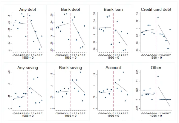
Figure 2: Treatment effect on household borrowing and saving measures by birth cohort

(43)

32

Table 10: Descriptive statistics (by marital status of the household head)

Married Unmarried

All Treatment Control All Treatment Control

(1) (2) (3) (4) (5) (6)

Mean Mean Mean Mean Mean Mean

Sd. Sd. Sd. Sd. Sd. Sd.

A – Educational outcomes

Junior high school 0.720 0.857 0.668 0.848 0.965 0.725

(0.449) (0.331) (0.471) (0.360) (0.185) (0.447) High school 0.539 0.560 0.533 0.717 0.823 0.606 (0.490) (0.497) (0.499) (0.451) (0.382) (0.490) College 0.279 0.262 0.284 0.520 0.611 0.424 (0.448) (0.440) (0.451) (0.500) (0.488) (0.495) B – Debt Any debt 0.393 0.393 0.393 0.288 0.297 0.279 (0.489) (0.489) (0.489) (0.453) (0.458) (0.449) Bank loan 0.336 0.323 0.339 0.254 0.354 0.253 (0.473) (0.470) (0.473) (0.436) (0.436) (0.435)

Credit card debt 0.097 0.094 0.098 0.091 0.081 0.100

(0.296) (0.292) (0.297) (0.287) (0.274) (0.301) C – Saving Any saving 0.157 0.154 0.158 0.217 0.237 0.197 (0.364) (0.361) (0.35) (0.413) (0.426) (0.399) Bank saving 0.080 0.083 0.079 0.138 0.159 0.115 (0.272) (0.275) (0.270) (0.346) (0.366) (0.320) Bank account 0.078 0.079 0.078 0.134 0.156 0.112 (0.269) (0.270) (0.268) (0.341) (0.363) (0.315) Other 0.002 0.003 0.002 0.005 0.004 0.007 (0.049) (0.057) (0.047) (0.074) (0.059) (0.086) D – Labor market outcomes

Employed 0.838 0.807 0.848 0.741 0.756 0.725 (0.369) (0.395) (0.358) (0.439) (0.430) (0.447) Wage earner 0.653 0.632 0.660 0.652 0.707 0.595 (0.476) (0.482) (0.474) (0.477) (0.456) (0.492) Private sector 0.662 0.642 0.668 0.493 0.452 0.535 (0.473) (0.477) (0.471) (0.500) (0.497) (0.500) E - Individual characteristics Age 32.11 26.69 33.94 29.61 25.56 33.86 (3.711) (1.842) (2.008) (4.632) (1.973) (2.135) Sex 0.851 0.816 0.863 0.580 0.633 0.524 (0.356) (0.388) (0.344) (0.494) (0.483) (0.500) Observations 2451 618 1833 552 283 269

(44)

33

Table 11: Effect of Reform on individual characteristics

Individual characteristics

(1) (2) (3) (4)

Employed Wage earner Private sector Married

A - Household heads Reform 0.032 0.027 0.045 0.048 (0.029) (0.041) (0.037) (0.035) Observations 3003 3003 3003 3003 B - Spouses Reform 0.049 -0.00031 0.053 (0.046) (0.048) (0.041) Observations 2025 2025 2025 Reform-spouse 0.011 0.024 0.013 (0.040) (0.038) (0.031) Observations 2179 2179 2179

Notes: Columns (1) and (2) report the effect of the treatment status of the household head and the spouses on their respective labor market outcomes. Column (3) reposts the effect of the treatment on the marriage market outcomes. The sample consists of individuals born between 1979 and 1993, with ages ranging from 22 to 37 years old. The dependent variables are Employed and Wage earner are indicator variables for the individual being employed and receiving a regular wage, respectively. Married is a dummy that takes 1 if the individual admits to being in a cohabiting relationship. Reform and Reform-spouse are dummy variables that take 1 if the household head or their spouse belongs to the treatment group, i.e. was born after 1986, respectively. The 1986 cohort is not included. The control variables include a dummy for having spent the first 15 years in a village, childhood and current residence fixed effects, control and treatment time trends and their interaction with the sex of the household head (or the spouse in the relevant specifications). The selected bandwidth is 7 (by the CCT algorithm). Standard errors are clustered at region-of-birth-by-birth-year level.

Quality versus quantity the limited impact of compulsory schooling laws on household financial behavior

ABSTRACT

ÖZET

ACKNOWLEDGEMENTS

TABLE OF CONTENTS

LIST OF TABLES

LIST OF FIGURES

CHAPTER 1

PRELIMINARIES

CHAPTER 2

EMPIRICAL STRATEGY

CHAPTER 3

MAIN RESULTS

CHAPTER 4

ROBUSTNESS

CHAPTER 5

CONCLUDING REMARKS

BIBLIOGRAPHY

APPENDIX