A class of adaptive directional image smoothing filters

(1)

Pergamon

_{Printed in Great Britain. All fights reserved} 0031-3203/96 $15.00+.00

PII:S0031-3203(96)00046-5

A CLASS OF ADAPTIVE DIRECTIONAL IMAGE

SMOOTHING FILTERS

M E H M E T i. GORELLi* and LEVENT ONURAL t

Department of Electrical and Electronics Engineering, Bilkent University, 06533 Ankara, Turkey

(Received

26

May

1994;

in revised form 6 March

1996;

received for publication 4 April

1996) Abstract--The gray level distribution around a pixel of an image usually tends to be more coherent in some directions compared to other directions. The idea of adaptive directional filtering is to estimate the direction of higher coherence around each pixel location and then to employ a window which approximates a line segment in that direction. Hence, the details of the image may be preserved while maintaining a satisfactory level of noise suppression performance. In this paper we describe a class of adaptive directional image smoothing f'llters based on generalized Gaussian distributions. We propose a measure of spread for the pixel values based on the maximum likelihood estimate of a scale parameter involved in the generalized Gaussian distribution. Several experimental results indicate a significant improvement compared to some standard filters. Copyright © 1996 Pattern Recognition Society. Published by Elsevier Science Ltd.

Adaptive filtering Directional filtering Image smoothing Median filtering Linear filtering

1. INTRODUCTION

Various nonlinear filtering techniques are shown to be useful for image processing applications. This is a consequence of the nature of the structural and statistical properties encountered in most common image types. It is also observed that common images cannot be modeled as statistically stationary signals. These observations lead to processing with adaptive filters.

What features of the adaptive filter will be changing as a consequence of the observed signal is, of course, the main issue. How these features will change by the observed signal is a very important problem, too. Usually the first problem is solved rather heuristically: the designer chooses those features which are most appropriate to the problem at hand, and while doing so, he tries to prefer those choices which have fewer number of adaptation parameters, and where the adaptation is tractable. Once the fixed and adaptive features of the filter are set, an adaptation algorithm can be found using analytical techniques. The adaptation speed is also an important issue: it is desirable to match the adaptation speed to the speed of the statistical and/or structural changes in the signal.

There are various adaptive nonlinear filters in the literature that are intended for image/video filtering applications. Some of these filters perform the adaptation by comparing the filter output with a reference signal, and then try to minimize a cost function of the difference of these two signals. ¢13-1s) In these applications it is assumed that a good sample of a desired signal

* Present Address. Signal and Image Processing Institute, Department of Electrical Engineering-Systems, University of Southern California, Los Angeles, CA 90089, U.S.A.

t Author to whom correspondence should be addressed.

is available to be used as the reference signal. Usually either the original uncorrupted image is used off-line during training or the corrupted signal itself is used hoping that the contamination will not change the adaptation process significantly. Furthermore, the filter structure is assumed to be convenient so that after the adaptation process it can perform the desired job. Many other applications collect signal statistics of some sort within a region, and then make decisions about the filtering procedure and/or the filter parameters based on these statistics. (3"16'~7'18) These type of filters usually require less computation. Here the assumption is that the desired behavior of the filter for a given statistics is known and such output is adequate for successful operation. Heuristics are used to select how and which statistics are going to be collected, and to decide about the consequent filter behavior.

In this paper, a class of adaptive directional image smoothing filters is developed based on the generalized Gaussian distributions. These filters may be put into the second group of filters mentioned above. The corresponding adaptive median and linear filters are presented as the special cases of this general class.

An interpretation of the median operation is as follows. (12) Suppose the data values are independent samples from a given Laplacian (also known as bi- exponential) distribution. That is, they have the common probability density function given as

f(x) = ~ e -Ix-'U~,

- < x ~ < x < c ~ . (1) Then the median filter output is the maximum likelihood estimate of the mean 7/of the distribution based on the data values. A similar interpretation also holds for the standard linear filter. If the pixel values contained inside 1995

(2)

the shifted window is modeled as independent samples from a given Gaussian distribution, that is

_

1 e_(ix_,l/3)2

f ( x ) - - ~

, - o o < x < c c . (2) then the standard linear filter output is the maximum likelihood estimate of the mean ~ of the distribution based on the pixel values inside the window.

The median filter usually gives better estimates of the distribution mean compared to the linear lowpass filter for images corrupted by impulsive noise. This is roughly because the Laplacian distribution has a larger tail weight compared to the Gaussian distribution. On the other hand the Ganssian distribution has a probability mass more concentrated around its mean value compared to the Laplacian distribution. Roughly speaking, this implies that the maximum likelihood estimate of the mean based on Gaussian distribution is less sensitive to relatively small noise components compared to the Laplacian distribution.

Although median filters usually preserve edges, both filters generally fail in preserving high frequency components such as texture and thin lines. The class of adaptive filters described in this paper is based on generalized Gaussian distributions which include both the Laplacian and Gaussian distributions as its special cases. The aim of the proposed class of filters is mainly to preserve high frequency components such as texture and thin lines while preserving the noise suppression properties of standard filters. Edge preserving filters have been studied by many researchers and interesting results have been obtained especially in the context of Kalman filtering. {6-11) In reference (11), neural network structures have been proposed for edge-adaptive Kal- man filtering. Furthermore, approaches that are similar to the one presented in this paper have been proposed independently by other researchers [see (19) and the references therein]. The idea presented in this paper has partially appeared in reference (4).

The organization of this paper is as follows. In Section 2, the generalized Gaussian distributions are described. In Section 3, a class of adaptive directional image smoothing filters is proposed. In Section 4, we present Monte Carlo simulations and experimental results. Finally, conclusions and comments are given in Section 5.

2. G E N E R A L I Z E D GAUSSIAN DISTRIBUTIONS

The

generalized Gaussian distribution

is a family of symmetrical probability distributions defined as

f~,3,v(x ) _

c~

e_(ix_,l/;~). - c ~ < x < exp. (3)

23r(~)

where F(.) is the gamma function, fl > 0 is the scale (spread) parameter, and c~ > 0 is the shape parameter. Also, ~/is the mean value of the distribution. This family of probability distributions has been used in detection theory and in deconvolution of seismic signals as models for non-Gaussian signals. (L2)

A wide and useful range of probability distributions can be obtained from the generalized Gaussian distribution by appropriately choosing the parameters. For c~ = 1, we have the bi-exponential distribution, also known as Laplacian distribution,

fL3,o(x)

= ~fl e Ixl/• -cx~ < x < c~. (4) For a = 2 we have the w e l l - k n o w n G a u s s i a n distribution,

f2,3,o(x) = l ~ e - ( r x l / 3 ) 2 ,

- o o < x < oo. (5)

x/~3

As a tends to infinity, we have the uniform distribution. For a generalized Gaussian distribution with mean z/ and parameters a and/3, the rth (centralized) absolute moment, defined as

f

cx~ r X # r = g { 1 2 - o l r } = I x - ~ l

fc,,3,n( ) d x

(6) to is given in (2),

r((r

+

1)/c~) fir.

# r - - F ( 1 / C ~ ) (7)

It can be shown that, as a increases, the scale invariant kurtosis defined as the ratio of #4 to the square of #2 dec reases.(2) This implies that as a gets larger, the distribution becomes more concentrated around its mean and also the tail weight decreases.

The variance 0 2 given by 0-2 = #2 is proportional to 3 2 for a given a. Hence /3 (or equivalently, 3 '~) is a measure of spread of the generalized Gaussian distribution. The joint maximum likelihood estimates of the mean ~ and the scale parameter 3 of these distributions can be easily computed: Given a set of independent observations

{ X l , . . . , X u }

from a given generalized Gaussian distribution with a given shape parameter a, the joint maximum likelihood estimates, ~ML and/3ML, of the mean r/and the parameter 3 are found as

N

~ML such that ~ [xi - ~)ML r is minimized, (8)

i-1

flML =

o~

I xi -- ¢IML t '~

(9)

N / = 1

In this paper, we will be mainly interested in cases a = 1 and c~ = 2, that is, Laplacian and Gaussian distributions, respectively. For c~ = 1, the estimates given above become,

~ML = M E D { x ~ , . . . ,

XN

}, (10)

1 s

flML = ~ .i~= 1 I Xi -- ~ML I " ( 1 1 )

where MED denotes the median operation. For c~ = 2, we have

1 re

¢IML = ~ ~ _ X i ,

(12)

(3)

m = l

4

[]

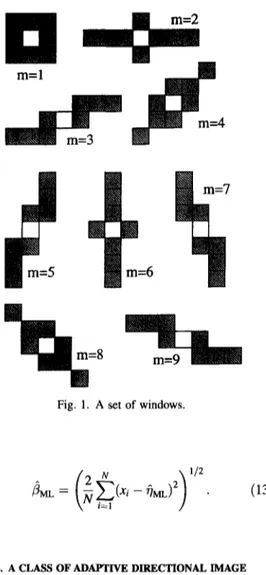
m = 6

m

= 8

Fig. I. A set of windows.

2 iv 1 / 2

(13)

3. A CLASS OF ADAPTIVE DIRECTIONAL IMAGE SMOOTHING FILTERS

The clarity of edges in images is very important. Smoothing is also desirable to eliminate disturbing noise. But usually, these requirements are contradictory. Any kind of smoothing must be based on a model behavior of groups of pixels. It is not a bad assumption if this grouping behavior is considered to be along lines. Under this assumption, it is expected that a pixel would be a part of a line of arbitrary gray level. The line is assumed to be straight at least for a few pixels, and its orientation is arbitrary. Such assumptions are used for lossy coding of images, and reported to be successful. (2°) The constant gray level requirement along a locally straight line is relaxed and it is assumed only that the pixels have a higher coherence in one direction compared to other directions. The outcome of these observations and assumptions is the adaptive directional smoothing filter presented in this paper. More specifically, we have a set of directional windows. At each pixel location, we measure the coherence of pixel values by a suitable criterion for each of the available windows. Finally, at a given pixel location, filtering is performed using the window which contains the most coherent data values.

For the mathematical development, we will denote the rectangular array of pixels by ~ . We will denote

images as x or y. The value of a pixel i E 9 will be denoted by a notation such as

x(i)

or

y(i).

We will consider a set of nine windows indexed as m = 1 , . . . , 9 as shown in Fig. 1. The windows for m --- 2 , . . . , 9 are chosen to approximate line segments in eight directions as shown in Fig. 2. The window with index m = 1 is a non-directional one to account for uniform regions. The non-shaded pixels are the window centers which may be shifted to an arbitrary pixel i E 9 . We will use the notation,

Wm.i,

m = 1 , . . . , 9, to denote a window of index m with its center shifted to pixel i E 9 . Furthermore, we will use the notation " ~ i to denote the set of all windows with their centers shifted to pixel i.

Consider an image x to be filtered. We define X,,./, as the set of pixel values contained inside the window

Wm,i,

that is

Xm, i

= {x(i) I i E

Wm,i}.

(14)

TO measure the coherence of pixel values in

Xm.i,

we will use a measure based on the maximum likelihood estimate/~rea, of the scale parameter/3. A simple method is to compute/~ML for each

X,,,.i,

m = 1 , . . . , 9 at a given pixel i E 9 , and choose the window that yields the smallest /~ML value. Note that (/~¢a~) ~ may be equivalently used instead of/~ML to measure the spread of the pixel values, since taking a positive power does not change the rank ordering of/~rea~'s.

In this paper, we will define a slightly more general measure of the spread of pixel values. This general- ization is based on the observation that the coherence direction in a given image is usually the same in spatially close pixels. In other words, if ~ i c 9 is neighborhood of pixel i, then we may expect that the coherence direction will be approximately the same at each pixel location in ~i. Based on this assumption, we define a spread parameter (m,i for the set of pixel values

Xm. i

as

1 ~ ^

_ (/3ML)m,j, (15)

where # / i , denotes the number of pixels in the set t i i). Also (/3rcm)~j, denotes the a t h

(including pixel power

of/~r~ given by (9) based on the observation of the data

m ~ ~ 7 n~=6 ~ =5 m - - 4 t m 9 N }k I I I / V ] m = 3

N \ I I I / V I t

I I 1 ~ 1

.'I

I IN

I/I /lllkl

/

I \

m = 2

4"

_\

Fig. 2. Eight directions that are used in selecting the directional windows.

(4)

values in the set Xmj. So we have the following definition.

Definition

1: Assume that the model parameter a is

chosen, and the image to be filtered is x. The value of the filtered image y at a given pixel i E ~ is given by

y(i)

= (OML)rh,i , (16)

where r h { 1 , . . . , 9} is such that

~Fn,i

~

~m,i

gm E { 1 , . . . ,9} (17) and (~ML)~,i is the maximum likelihood estimate of ~/ given by (8) based on the observation of the data values in the set

X~,i.

Remark.

For ~ i = {i}, the filter output

y(i)

at pixel i (assuming a is fixed) minimizes the cost function g(y(i)) given by

g(y(i))

= m i n / Z

I x ( j ) - y(i)1~1 m - - 1 , . . . , 9 } .

kjEWm,i

(18) For other choices of ~ , a compact form of the cost function may be more complicated.

If the model parameter a is chosen as 1, then we obtain an adaptive directional median filter for which Definition 1 is restated as follows.

3.1. The adaptive directional median filter

For a given input image x, the filter output at a pixel i E ~ is given as

y(i)

= MEDX,~,i (19)

where rh is as def'med in (17) and the spread parameter

~m,i

given by (15) can be written as

~m,i --

Z

I x ( k ) - (~L)m,j I •

i

kEWm,j

(20) Note that if the set ~ i includes the pixel i only, that is if ~ i = {i}, then

~m,i

given by (20) reduces to

1

~ra,i -- #Wm, i Z

Ix(k)

- (~]ML)m,i

I " (21)

k6Wm,i

Remark.

If the image is corrupted by very spiky noise components, then some of the terms in the inner summation in (20) may be very large which will increase the value of

~m.i.

In this case, omitting a number of largest terms in the inner summation in (20) may increase the filter performance. The modified form of

~m,i

will be

1 ~ / 1

~m,~ - ~ j ~ , l # W m j -- A

#W~,j-A }

Eth smallest{[

x(k) - (¢haL)m~

[I

k ~ Wmj} •

gel

(22) where A is the number of discarded terms in the inner

summation. Note that for A = 0, the def'mition in (22) reduces to (20).

If the model parameter a is chosen as 2, then we obtain the adaptive directional linear filter defined as follows.

3.2. The adaptive directional linear filter

For a given input image x, the filter output at a pixel i E ~ is given as

1

y(i) --

Z x(j)

(23)

#w~,,,

_jEW~n,i

where rh is as defined in (17) and the spread parameter

(m.i

given by (15) can be written as

# ~ i 1 jet, i{

#Wm,j

1

-

2 }

~m,i --

~

(X(t) -- (~ML)m,j)

kEWm, j

(24) Note that if ~ i = {i}, then

~m.i

given by (24) reduces to

1 ~ 2

-- -- ((~)ML)m,i}

(,,,i Z {x(k) . (25)

#Wm,i

_kEW~.~

The choice of a is roughly a compromise between three major criteria: computational concerns, noise suppression properties, and pattern preserving properties. Among the computational concerns is the minimization of the function in (8) to obtain OML" For a < 1, the function is not convex, however its minimum always occurs at one of the data values. For a >_ 1, it is convex and can be minimized by a gradient descent method. For a = 1 and a = 2, closed form expressions are given by (10) and (12), respectively. For discrete valued images (which is the case in practical applications), the minimization is carried out over a finite domain which may reduce complexity. Noise suppression properties are also an important factor in the choice of a. As cz gets larger, the generalized Gaussian distribution becomes more concentrated around its mean value and its tail weight decreases. This phenomena may be observed from the scale invariant kurtosis ( = (#4/(#2)2). (2) Roughly speaking, this implies that as a gets larger, ¢tML becomes more sensitive to large noise components in the data and less sensitive to small noise components. For this reason, for impulsive noise, choosing a small value for a is suitable, whereas for Ganssian noise with small variance, a larger value of a is generally better. Note that in practice, median filters are preferred to linear lowpass filters for impulsive noise cancellation. Finally, an important criterion may be the pattern preserving properties. It is well known that median filters are superior to linear filters in preserving sharp edges. For the adaptive directional filter proposed in this paper, pattern preserving is enhanced both for the median and linear filters.

3.3. Salt-and-pepper noise

Up to now, it was assumed that noise components were distributed by generalized Gaussian distribution.

(5)

Here we will define a specific form of salt-and-pepper

noise [this model is in part inspired by Problem 12, Section 3.3 of (21)]. Assume that a pixel value is contaminated by an independent noise component with probability p, otherwise it is noisefree. Then the distribution of the pixel value will be (by allowing impulse functions)

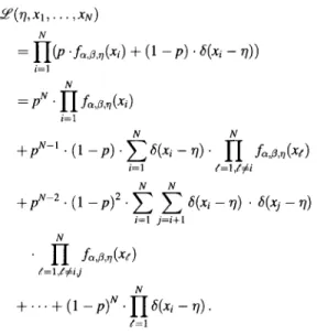
g~,g,,,,p(X) = p . fa,g,o(x) + (1 - p) . 6(x - r/), (26)

where fagm(x) is the generalized Gaussian distribution. In this distribution, ~7 represents the underlying noiseless pixel value. Given a set of data values { X l , . . . , xu} from the above distribution, the ML estimate ~ML of the mean 77 maximizes the likelihood function

~e(~, x i , . . . ,

XN)

N = H ( p .fa,Ao(xi) + (1 - p ) . ~(x i -- 71)) i=1 N

= PN" H io,j,.(x,)

i=1 N N

_~_pN-l. (1 --p)"

Z ~ ( X i -

'/7)'

H

f°~'g'r#(X~#)

i=1 ~ ' = 1 , ~ i N N + p N - 2 . (1 _ p ) 2 . Z Z 6(xi -- rl) • 6(Xj -- rl) i=1 j = i + l N

H

,f=l,~TLij N + . . . + (1 - p)N. H e(xi - - 77)" d = l (27) From the above equation, the following results may be obtained for salt-and-pepper type of noise distributed according to (26). If none of the data values are equal, then the terms containing two or more 6-functions will vanish, hence ~o will be dominated by the terms containing a single 6-function. Therefore, if xi ¢ x;Vi,j

such that i ¢ j, then

N

7 ) M L m i n i m i z e s

Z

I

X i - - 7]ML I cx

i : I ( 2 8 )

such that 7)i L E { x i , . . . , x u } .

That is, ~Im minimizes the same function given in (9), except that, now it is constrained to be minimized over the set { x l , . . . ,XN}. Note that, for c~ < 1, the minimum already occurs at one of the data values, hence for a < 1 and with the assumption that all data values are different from each other, it is concluded that for all 0 < p < 1, the ML estimate OML is given by (8). Another result that can be obtained from (27) is that if two or more data values are equal and the others are all different, then ~ML is equal to that value that is observed more than once.

Note also that, for p = 1 we obtain a pure generalized Gaussian distributed noise, hence the above model is a more general one.

4. SIMULATIONS AND RESULTS

The class of adaptive directional filters described in Section 3 consists of two steps: First, the directivity is estimated, then filtering is performed. The estimation of directivity is a multiple hypothesis testing problem, the best window is selected from a given set of directional windows. In this section, the performance of directivity detection will be studied, and the experimental results will be given for real images.

4.1. Directivity detection

In this section, the probability of correctly detecting the directivity will be studied through Monte Carlo tests performed over synthetically generated data.

The set-up for the image model is as follows. The image is defined on a two-dimensional (continuous) coordinate system where the horizontal and vertical coordinates are labeled by u and v, respectively. We consider the directivity in the neighborhood of the origin as shown in Fig. 3. The eight directions shown in Fig. 3 are the hypotheses to be tested. Without loss of generality, the true directivity is chosen to be along the horizontal axis (that is, direction 1 in Fig. 3). The image is described locally as a zero-mean, unity variance Gaussian random field which is constant along the horizontal axis, and has the covariance function

C ( Y l ~ V 2 ) = e Ivl v21/0.4 (29) where vl and v2 are the vertical coordinates of two arbitrary points (as a reference for distance, the radius of the outermost circle in Fig. 3 is chosen to be unity). Each of the eight windows contain nine points as indicated in Fig. 3.

The image is contaminated by additive, independent, identically distributed salt-and-pepper type of noise described by (26) with the mean ~7 set to zero. In order not to confuse the parameters involved in the noise distribution by those involved in the spread parameter, we adopt the following notation: The symbols & and/3

V

6\_. 5

... , I X

8/.

"~.,_ .... 4 / i ... J- .... 3 ... ... . / . S / ... / " : / ; ... 2 ...

... :;I'"':T i i l

91 . i . , , ~ ~ , ... U " "..."" {'-"~'. " ' ~ ... i ... : ) U

(6)

(b)

(A)

"'''''"'--.

i a .. " ' - . . . . . o • "o. I 2 S l (B) t

i.i

i , - . . . :-.- . . . o. ....

2

o; o.o x ~ ~t

(c)

_(D)

I 2 $ o, tta o.7

(c)

(d)

"k ' 0 " M e t h o d 1: M e t h o d 2: Pt 07 " , " ' , " . . ' ' . , [ " ' . M e t h o d 5 : - - 1 9 - - - M e t h o d 6: M e t h o d 3: ... M e t h o d 4: X

Fig. 4. Probability of correctly detecting the directivity [P (correct)] versus noise scale parameter, # Columns: (A) p = 0.2, (B) p = 0.5, (C) p = 0.8, (D) p = 1.0. Rows: (a) & = 0.5, (b) ~ = 0.75, (c) ~ = 1.0, (d) = 2.0. In all plots, the vertical axis denotes P(correct) and ranges from 0 to 1. The horizontal axis represents #

and ranges from 0 to 4. will denote the true values o f the shape and scale

parameters o f the noise distribution. The variables a and will denote the assumed shape and scale parameters used in computing the spread parameter and ~ML.

Because o f the way the image field is described, the true hypothesis is direction 1 in Fig. 3. Several Monte

Carlo test results will be presented for various parameters o f the noise distribution and various choices o f the spread parameter. The curves of the probability of correctly detecting the directivity versus noise level are presented in Fig. 4. Each plot i s obtained by averaging over 10,000 pseudorandom realizations of

(7)

the above described image model for each different choice of the model parameters. In Fig. 4, each plot represents the probability of correctly detecting the directivity as a function of the scale parameter/~ of the additive

salt-and-pepper

noise distribution given by (26). The plots in columns (A), (B), (C), and (D) of Fig. 4 correspond to p = 0.2, 0.5, 0.8, 1.0, respectively. The plots in rows (a), (b), (c), and (d) correspond to & = 0.5,0.75, 1,2, respectively. Each plot contains six curves corresponding to six different methods of estimating directivity. These methods are as follows: In Methods 1-5, the spread parameter given by (15) is used with ~ i = {i} with c~ = 0.3,0.5,0.8, 1,2, respectively. That is, the spread parameter is given by

N

Xm,i = ~ [ Xi -- OML [c~, OZ = 0.3, 0.5, 0.8, 1.0, 2.0 i=1

(30) and N = 9 in this case. In Method 6, the spread parameter is chosen as in (22) with ~ i = {i} and A = 2. It is observed in Fig. 4 that smaller values of a in the spread parameter yields a higher probability for correctly detecting directivity. Note that Method 6 yields a performance comparable to that of Methods 1 and 2 in which relatively small values of ct were used. Furthermore, Method 6 involves only absolute value and rank ordering operations, whereas the other methods involve computation of powers. For this reason, Method 6 seems to be more suitable for hardware implementa- tion. Another fact to note is that, as p ~ 1, all methods yield approximately the same performance.

An intuitive explanation for the performance of Method 6 for p < 1 may be as follows. Since some of the largest terms in (22) are omitted, the corresponding spread parameter roughly chooses the direction in which all, except for a few, pixel values take on very close

i

values. Note that this coincides with the fact that if two or more data values are the same in a

salt-and-pepper

type of noise, then the common value of those data will be the estimate for the mean.

4.2. Experimental results

In this section, some experimental results will be given to demonstrate the performances of the adaptive directional median and linear filters based on both subjective and objective criteria. Subjective testing involves visually analysing the features of the obtained images. Objective testing is based on computing the mean squared error (MSE) between the original image x and the filtered image y. The MSE is defined as

MSE =

~ - ~ ~-~(y(i) - x(i)) 2 .

(31)

(a)

Fig. 5. Original "baboon" image.

(b)

Fig. 6. (a) Standard median filter output using 3 x 3 window, (b) the adaptive directional median filter output.

(8)

ga

t~

800 700

600

500 IStSE

curv~ ( ~ " I )

4(101-

/ / / A

T~/ : 9 x 9 A : 2 "/-4i : 9 × 9 A : 0 ....

..'"

~ S M F ..-"' .,"

T~

: l x l

..."

~'ji'"'/""

"

: o

.-:;:"~;-

. /

1

,..""

J

.,.."

300 ~

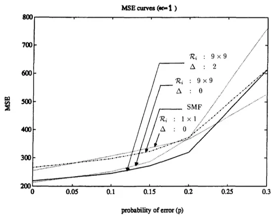
... :::::::::::::::::::::::"t::r""- ... J ... 2 0 0 ~ 0 0.05 0.1 0.15 0.2 0.25 0.3 tn~bability o f e r r o r (p)

Fig. 7. MSE curves for various choices of ~i and A plotted as a function of probability of error p.

For the test results given in this section, we used the "baboon" image shown in Fig. 5. The pixels are represented by eight bits.

4.2.1. The adaptive directional median filter. To see the distortion introduced by the filtering operation, the (noiseless) image is filtered both by the adaptive directional median filter (ADMF) which uses the 9 windows shown in Fig. 1, and by the standard median filter (SMF) which uses a 3 x 3 window. The SMF output and the ADMF output are shown in Fig. 6(a) and (b), respectively. A considerable improvement in the textured regions and thin lines is observed in the ADMF output. The ~ i in (2) is chosen to be 9 x 9 pixel array centered at pixel i.

The MSE values for several noise levels and several choices of the variables involved in (22) are shown in Fig. 7. The horizontal axis is the probability p that a pixel value is erroneous. More specifically, pixels of the original image are chosen with probability p and the value of the chosen pixel is converted to either 0 or 255 with equal probabilities of 0.5. In Fig. 6, the SMF curve corresponds to the standard median filtering with a 3 × 3 window. The other curves are the ADMF results for several different choices of ~ i and A. Remember that for A = 0, the spread parameter given by (22) reduces to the one given in (20). Observe that for smaller values of p, suitably larger choices for ~ i reduce the MSE. For larger values of p, the MSE is still reduced

by choosing A suitably larger than zero. This latter effect is intuitively due to the fact that the noise process being used is too spiky to be modeled by Laplacian distribution (a = 1). A smaller value of a might be more suitable. As an alternative, the modification of the spread parameter given in (22) may be used. Omission of some of the largest terms in (20) suitably modifies the value of the spread parameter ~m,i which eventually results in a better estimation of the coherence direction. Since the median operation is quite robust for isolated large errors in data values, the overall MSE decreases. Therefore, modification of ~,,,i in (20) by omitting some large terms as in (22) may be an alternative to choosing a < 0 which might bring a great deal of computational complexity.

4.2.2. The adaptive directional linear filter. The

testing of the adaptive directional linear filter (ADLF) proceeds in a manner similar to that of ADMF. In Fig. 8(a) and (b), the outputs of standard linear filter (SLF) which employs averaging over a 3 x 3 window and A D L F are shown. A g a i n , a c o n s i d e r a b l e improvement in the texture and thin lines is obtained by using ADLF.

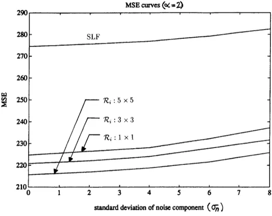
In Fig. 9, four MSE curves are plotted. As the noise process, we used an additive white Gaussian process (suitably approximated to take on integer values) with standard deviation ~r n. As seen in Fig. 8(a), the SLF has a higher MSE compared to ADLE As the size of ~ i is

(9)

m

(a) (b)

Fig. 8. (a) Standard linear filter output using 3 x 3 window, (b) the adaptive directional linear filter output.

MSE curves ( ~ - 2 )

290 28O

270

260

2.50

240

230

220 ~

210

0

S L F

¢

T~i : 5 x 5 T~i : 3 x 3 "R.i : 1 x 1

standard deviation of noise component (&n)

Fig. 9. MSE curves for various choices of ~i plotted as a function of noise standard deviation a n.

increased, the MSE gets even smaller. Since the noise process is approximately Gaussian, we do not use an approximation of the spread parameter ~m,i by omitting large error terms.

5. C O N C L U S I O N

In this paper, a class of adaptive directional image smoothing filters is described. In particular, the

implications of the proposed model on median and linear filtering are emphasized. Both subjective (based on visually comparing the images) and objective (based on MSE criterion) testing of the adaptive directional median and linear filters revealed considerable enhance- ment compared to the standard median and linear filters. Another interesting observation is that the heuristic approach described by (22) performs very well under

(10)

REFERENCES

1. J. H. Miller and J. B. Thomas, Detectors for discrete-time signals in non-Gaussian noise, IEEE Trans. Inf. Theory IT- 18(2), 241-250 (March 1972).

2. W. C. Gray, Variable norm deconvolution, Ph.D. Disserta- tion, Stanford University (August 1979).

3. G. R. Arce and M. P. McLoughlin, Theoretical analysis of the max/median filter, IEEE Trans. Acoust. Speech Signal Process. 35(1), 60-69 (January 1987).

4. M.i. Gtirelli and L. Onural, The adaptive directional median filter, Proc. Sixth Int. Symp. Comput. Inf. Sciences, Side, Antalya, Turkey, 973-979 (October 30-November 1991). 5. M. P. McLoughlin and G. R. Arce, Deterministic properties

of the recursive separable median filter, IEEE Trans. Acousr Speech Signal Process. 35(1), 98-106 (January 1987). 6. J. W. Woods and C. H. Radewan, Kalman filtering in two

dimensions, IEEE Trans. Inf. Theory 23(4), 473-482 (July 1977).

7. M. S. Murphy and L. M. Silverman, Image model representation and line-by-line recursive restoration, IEEE Trans. Automatic Control 23(5), 809-816 (October 1978). 8. J. W. Woods and V. K. Ingle, Kalman filtering in two

dimensions: Further results, IEEE Trans. Acousr Speech Signal Process. 29(2), 188-197 (April 1981).

9. A. M. Tekalp, H. Kaufman and J. W. Woods, Edge-adaptive Kalman filtering for image restoration with ringing suppression, IEEE Trans. Acousr Speech Signal Process

37(6), 892-899 (June 1989).

10. M. R. Azimi-Sadjadl and S. Bannour, Two-dimensional recursive parameter identification for adaptive Kalman filtering, IEEE Trans. Circuits Syst. 38(9), 1077-1081 (September 1991).

11. R. Xiao and M. R. Azimi-Sadadl, Neural network decision directed edge-adaptive Kalman filter, IEEE Int. Conf. Neural Net. 4084--4089 (1994).

12. J. Astola, P. Haavisto and Y. Neuvo, Vector median filters,

Proc. IEEE 78(4), 6784589 (1990).

13. L. Yin, J. T. Astola and Y. A. Neuvo, Adaptive stack filtering with application to image processing, IEEE Trans. Signal Process. 41(I), 162-184 (January 1993). 14. P. Salembier, Adaptive rank order based filters, Signal

Process. 27, 1-25 (1992).

15. J.-H. Lin, T. M. Sellke and E. J. Coyle, Adaptive stack filtering under the mean absolute error criterion, IEEE Trans. ASSP 38(6), 938-954 (June 1990).

16. A. Restrepo and A. C. Bovik, Adaptive trimmed mean filters for image restoration, IEEE Trans. ASSP, 36(8),

1326-1337 (August 1988).

17. H.-M. Lin and A. N. Jr. Wilson, Median filters with adaptive length, IEEE Trans. Circuits Syst. 35, 675-690 (June 1988).

18. L. Onural and M. B. Alp, Weight selection for the 2-D Adaptive Weighted Median Filter Based on the Gibbs Random Field Model, 1993 IEEE Winter Workshop on Nonlinear Digital Signal Processing, Tampere, Finland, 5.1-1.1-5.1-1.6 (January 1993).

19. P. Bolon, A Family of NL-Filters, 1993 IEEE Winter Workshop on Nonlinear Digital Signal Processing, Tam-

pere, Finland, 1.2-1.1-1.2-1.5 (January 1993).

20. Y. Wang and S. K. Mitra, Image representation using block pattern models and its image processing applications, 1EEE Trans. Pattern AnaL Mach. lntell. 15, 321-326 (April 1993).

21. Bickel and Doksum, Mathematical Statistics. Prentice- Hall, New Jersey (1977).

About the Author - - MEHMET ]ZZET Gf]RELLI received the B.S. degree in Electrical and Electronics Engineering from Middle East Technical University, Ankara, Turkey in 1987 and the M.S. degree in Electrical and Electronics Engineering from Bilkent University, Ankara, Turkey in 1990. From 1987 to 1991 he was a Research Assistant at Bilkent University. He is currently working toward the Ph.D. degree in Electrical Engineering at the University of Southern California, Los Angeles where he is a research assistant. His research interests include statistical signal processing, multichaunel system identification and blind deconvolution, communication theory, image processing, and image modeling using random fields.

About the Author - - LEVENT ONURAL received the B.S. and M.S. degrees in Electrical Engineering from Middle East Technical University, Ankara, Turkey in 1979 and 1981, respectively and the Ph.D. degree in Electrical and Computer Engineering from State University of New York at Buffalo in 1985. He was a Fulbright scholar between 1981 and 1985. After a Research Assistant Professor position at the Electrical and Computer Engineering Department of State University of New York at Buffalo, he joined the Electrical and Electronics Engineering Department of Bilkent University, Ankara, Turkey, where he is a Professor at present. He visited the Electrical and Computer Engineering department of University of Toronto on sabbatical leave in 1994. His current research interests are in the area of image and video processing with emphasis on very low bit rate video coding, texture modeling, non-linear filtering, holographic TV and signal processing aspects of optical wave propagation. Dr Onural is a senior member of IEEE. He was the organizer and the first chairman of IEEE Turkey Section. He is now the chairman of IEEE Region 8 Student Activities Committee.