Discriminating between the Lognormal and Weibull Distributions under Progressive Censoring

(1)

Cumhuriyet Science Journal

CSJ

e-ISSN: 2587-246X

ISSN: 2587-2680 Cumhuriyet Sci. J., Vol.40-2 (2019) 493-504

Discriminating between the Lognormal and Weibull Distributions under

Progressive Censoring

Coşkun KUŞ 1* _{, Ahmet PEKGÖR}2 _{, İsmail KINACI}3

1_{Selcuk University, Faculty of Science, Department of Statistics, Konya, TURKEY} 2_{Necmettin Erbakan University, Faculty of Science, Department of Statistics, Konya, TURKEY}

3 _{Selcuk University, Faculty of Science, Department of Actuarial Sciences}_,_{Konya, TURKEY}

Received: 12.10.2018; Accepted: 19.12.2018 http://dx.doi.org/10.17776/csj.470148

Abstract. In this paper, the ratio of maximized likelihood and Minimized Kullback-Leibler Divergence methods are discussed for discrimination between log-normal and Weibull distributions. The progressive Type-II right censored sample is considered in the study. The probability of correct selections is simulated and compared to investigate the performance of the procedures for different censoring schemes and parameter settings.

Keywords: Discrimination, Log-normal distribution, Power analysis, Simulation, Progressive type-II right censoring.

İlerleyen Tür Sansür Altında Lognormal ve Weibull Dağılımlarının

Ayrımı

Özet. Bu çalışmada, log-normal ve weibull dağılımları arasında ayırım için en çok olabilirlik oran ve

Kullback-Leibler uzaklık metotları tartışılmıştır. Çalışmada, ilerleyen tür sansürlü veri durumu ele alınmıştır. Doğru seçim oranları hesaplanmış ve farklı parametre ve sansür şemaları altında testlerin performansları karşılaştırılmıştır.

Anahtar Kelimeler: Ayırım, Log-normal dağılım, Güç analizi, Simülasyon, İlerleyen tür sansürleme.

1. INTRODUCTION

A discrimination procedure focus on making suitable selection from two or more distributions based sample. In other words, discrimination procedure tries to get decision on which distribution is more effective to modeling the data. A lot of papers in the literature on discrimination two or three distributions. Most of them are based on Kullback-Leibler Divergence (KLD) and ratio of maximized log-likelihood (RML). There are a lot of works in this area. Some of them are Alzaid & Sultan [1], Kundu & Manglick [2], Bromideh and Valizadeh [3], Dey and Kundu [4], Dey and Kundu [5], Kundu [6], Kantam et al. [7], Ngom, et al. [8], Ravikumar and Kantam, [9], Qaffou and Zoglat, [10] and Algamal [11].

In this study, we consider on discrimination between log-normal and Weibull distributions. The probability density function (pdf) of log-normal and Weibull distribution are given, respectively, by

(2)

Kuş et al. / Cumhuriyet Sci. J., Vol.40-2 (2019) 493-504

 

x

I

_ _

 

x

f

_

































₀_, 2

log

2

1 exp

2

1









 and

 

x x x I 

 

x g                    1 ₀_, exp 2   







where

I

_A

 

x

is an indicator function on set

A

and 1 





,





 and











,



2

 are distribution parameter vectors.

Some papers related the discrimination between log-normal and Weibull distributions are Quesenberry & Kent [12], Dumonceaux & Antle [13], Pasha et al. [14], Dey & Kundu [4,5], Bromideh [15], Raqab, et al. [16] and Elsherpieny et al [17]. Quesenberry & Kent [12], proposed selection statistic that is essentially the value of the density function of a scale transformation maximal invariant. They considered include the exponential, gamma, Weibull, and lognormal. Note that this method works only complete sample case. Dumonceaux & Antle [13] used the difference of the RML, in discriminating between the Weibull or Log-Normal distribution based on complete sample. Kundu & Manglick [18] obtained the asymptotic distribution of the discrimination statistic RML and determined the probability of correct selection (PCS) by using asymptotic distribution in this discrimination process. Dey and Kundu [19] extended the Kundu & Manglick [18]'s results to Type-II censored sample case. Pasha et al. [14] used RML and most powerful invariant for discriminating these distributions based on complete sample. Kim & Yum [20] extended to Pasha et al. [14]'s results to Type-I and Type-II censored sample cases. Dey & Kundu [4, 5] used the RML, in discriminating between the Weibull, Generalized Exponential Distributions or Log-Normal distribution based on complete and Type-I censored sample. They obtained the asymptotic distribution of the discrimination statistic and determined the PCS by using asymptotic distribution in this discrimination process. Bromideh [15] examined the use the KLD in discriminating either the Weibull or Log-Normal distribution based on complete sample. Raqab, et al. [16] used the RML, in discriminating between the Weibull, Log-logistic or Log-Normal distribution based on doubly censored sample. Elsherpieny et al. [17] considered test based RML and Ratio Minimized Kullback-Leibler Divergence RMKLD for discrimination between Gamma and Log-logistic Distributions based on progressive Type-II right censored data. The model of progressive Type-II right censoring is of importance in the field of reliability and life testing.

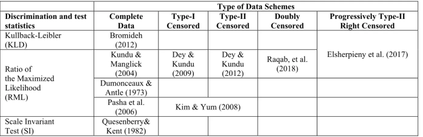
Table 1. The papers related to discrimination between lognormal and Weibull distribution Type of Data Schemes Discrimination and test

statistics Complete Data Censored Type-I Censored Type-II Censored Doubly Progressively Type-II Right Censored

Kullback-Leibler (KLD) Bromideh (2012) Elsherpieny et al. (2017) Ratio of the Maximized Likelihood (RML) Kundu & Manglick (2004) Dey & Kundu (2009) Dey & Kundu (2012) Raqab, et al. (2018) Dumonceaux & Antle (1973) Pasha et al.

(2006) Kim & Yum (2008) Scale Invariant Quesenberry&

(3)

All the papers except for Elsherpieny et al. [17], consider complete or Type-I and Type-II censored sample. In this work, we consider discrimination under progressive Type-II right censored schemes. Progressive Type-II right censoring scheme is explained as follows: Let n identical units are subject to a lifetime test.

r

_i surviving units are randomly withdrawn from the test,

1 

i



m

as soon as

i

-th failure is occured. Hence, if m failures are observed then

r

₁







r

_m units are progressively Type-II right censored; Thus,

n



m



r

₁







r

_m. Let

X

_{1: :}r_{m n}



X

_{2: :}r_{m n}



_



X

_{m m n}r_{: :} _{be the progressively Type-II}

right censored failure times, where

r





r

₁

,



,

r

_m



denotes the censoring scheme for the life test. As a special case if

r





0 

,

0 

, ordinary order statistics are obtained[21]. If

r





0,...,0, m



, the progressive Type-II right censoring becomes type-II censoring. For more details please see [22,23,24].

In this paper, the discrimination methods are given in Section 2. In Section 3, PCS are simulated by Monte Carlo methods and results are discussed. Finally, a numerical example is provided to illustrate the methodology.

2. RULES OF DISCRIMINATION

Let

X

_{1: :}r_{m n}



X

_{2: :}r_{m n}



_



X

_{m m n}r_{: :} _{are progressive Type-II right censored sample from log-normal}





_,





distribution. Then log-likelihood function [26] is given by

 



₁



₁   _, log log log 1 1 1 1                                      



  













i i m i i m i i m i LN x r x x m L  (1)

where



and



denotes the pdf and cdf of a standard normal distribution. Hence, ML estimate (it is denoted by

θ = μ,σ

ˆ

₁

 

ˆ ˆ

) of



₁can be obtained numerically which maximize the likelihood function (1). Let

X

_{1: :}r_{m n}



X

_{2: :}r_{m n}



_



X

_{m m n}r_{: :} _{are progressive Type-II right censored sample from Weibull}





_,





distribution. Then the log-likelihood function (see [27]) is given by

 

log

 

log

  

1



log

 



1



.

1 1 2 









_           



  i i m i i m i W x r x m m L  (2)

Hence, maximum likelihood (ML) estimate of



₂(it is denoted by

θ

ˆ

₂



 

 

ˆ,

ˆ

) can be obtained numerically which maximize the likelihood function (2).

One of the rules of discrimination is ratio of the maximized likelihood



RML



.

The ratio of maximized likelihood is defined as follows

   

ˆ

LN W

RML L



θ

₁



L

θ

₂

(4)

where

L

_LN

 



₁ and

L

_W

 



₂ are defined by (1) and (2), respectively and

θ

ˆ

₁ and

θ

ˆ

₂are ML estimates of 1



and



₂. If the

RML



0

then log-normal distribution is selected for the modeling data otherwise Weibull distribution is selected against log-normal distribution.

Second one is based on Kullback-Leibler divergence. The KLD is a non-symmetric measure of the difference (dissimilarity) between two probability distributions

1  f and 2  g . Kullback-Leibler divergence between models is defined by





 

_{ }

 



 



 



 



1 1 2 1 2 1 1 1 2 0 0 0 , log log log .       _ _    



         f x D f g f x dx g x f x f x dx f x g x dx It is noted that the





2 1, 

 g

f

D can also be written by



f

g



H

 

f

 

x



g

 

x



dx

D

₁

,

₂ ₁ ₁

log

₂ 0     









where

 

1  f H is Shannon's entropy of 1  f defined as

 

log



 



.

1 1 1 0

dx

x

f

x

f

H

_



_ _ 





It is well known that D



f_₁,g_₂



0 and the equality holds if and only if

( )

1 2 f_ x =g_ x , almost surely [28], [29]. Furthermore,





2 1,   g f

D can be considered to serve as a measure of disparity between

1  f and 2  g .



f1,g2



D denotes the "information lost when

2  g is used to approximate 1  f . Namely, KLD is a measure of inefficiency of assuming that the distribution of population is

2



g when the underlying distribution is 1  f . The smaller





2 1,   g f D means that 1 

f is selected and large values of





2 1,   g f D favor 2  g [15]. Let 1  f and 2 

g are probability density functions of log-normal and Weibull distribution respectively.

Then





2 1,   g f D and





2, 1 D g_ f_ are given by





 

_{ }

)) 2 ( 2 / 1 exp( ) log( ) log( ) log( ) log( 2 / 1 ) 2 log( 2 / 1 2 / 1 log , 2 0 2 1 1 2 1





















 _                    



dx x g x f x f g f D      496

(5)





 

_{ }

 

).

/

)

6

12

6 )

2 log(

6 )

log(

6 )

log(

12 )

log(

12 )

log(

12 )

log(

12 )

log(

6 (

12 /

1 (

/

)

log(

)

log(

(

log

,

2 2 2 2 2 2 2 2 2 2 2 2 2 2 2 2 2 2 0 1 2 2 1 2





































































































dx

x

f

x

g

x

g

f

g

D

    



f1,g2



D and





2, 1

D g_ f_ were given by Bromideh [15] but they cannot read clearly in their paper. Therefore, these equations are obtained using by Maple. Second method for discrimination is the ratio of Minimized Kullback-Leibler Divergence



RMKLD



rule (Elsherpieny et al., [17]) which is defined by







1 2



2 1 ˆ ˆ ˆ ˆ , log , D f g RMKLD D g f          _ _    

If

RMKLD



0 ,

then we select the log-normal distribution for modeling data otherwise we select the Weibull distribution for modeling data.

3. SIMULATION STUDY

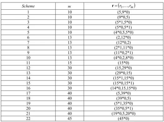
In this section, the PCS of RML and RMKLD methods are obtained and compared for different censoring schemes. The censoring schemes used in simulation are given in Table 2. Probabilities of correct selection of rules are simulated and given in Table 3-4.

Table 2. The censoring schemes used in simulation

Scheme m r



r1,,rm



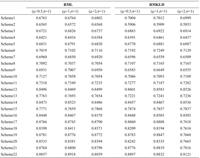
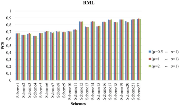
1 10 (5,9*0) 2 10 (9*0,5) 3 10 (5*1,5*0) 4 10 (5*0,5*1) 5 10 (4*0,5,5*0) 6 13 (2,12*0) 7 13 (12*0,2) 8 13 (2*1,11*0) 9 13 (11*0,2*1) 10 13 (4*0,2,8*0) 11 15 (15*0) 12 30 (15,29*0) 13 30 (29*0,15) 14 30 (15*1,15*0) 15 30 (15*0,15*1) 16 30 (14*0,15,15*0) 17 40 (5,39*0) 18 40 (39*0,5) 19 40 (5*1,35*0) 20 40 (35*0,5*1) 21 40 (19*0,5,20*0) 22 45 (45*0)

Let us consider the data come from log-normal distribution. From Fig. 1 and Fig. 2 the PCS of the RML and RMKLD are similar in general but the PCS of RML and KLD is slightly better than the PCS of other for some schemes. The selection of parameter values does not affect to the PCS so much.

497 498

(6)

Secondly, the PCS of the RML and RMKLD are better when the censoring is made at the beginning of the life test.

Now let us consider the data come from Weibull distribution. From Fig. 3 and Fig. 4 the PCS of RMKLD is better than the power of RML for all schemes. Secondly, the PCS of the KLD are better when the censoring is made at the end of the life test. The PCS of the RML are better when the censoring is made at the beginning of the life test.

Table 3. Probability of Correct Selection of RML and RMKLD rule when the data come from log-normal distribution

RML RMKLD (µ=0.5,σ=1) (µ=1,σ=1) (µ=2,σ=1) (µ=0.5,σ=1) (µ=1,σ=1) (µ=2,σ=1) Scheme1 0.6763 0.6764 0.6802 0.7004 0.7012 0.6999 Scheme2 0.6565 0.6572 0.6568 0.5906 0.5909 0.5853 Scheme3 0.6721 0.6826 0.6737 0.6883 0.6922 0.6914 Scheme4 0.6421 0.6416 0.6384 0.6391 0.6461 0.6437 Scheme5 0.6831 0.6791 0.6820 0.6770 0.6881 0.6887 Scheme6 0.7019 0.7102 0.7116 0.7192 0.7249 0.7129 Scheme7 0.6960 0.6850 0.6920 0.6596 0.6559 0.6509 Scheme8 0.7092 0.7037 0.7054 0.7107 0.7165 0.7165 Scheme9 0.6931 0.7007 0.6950 0.6583 0.6649 0.6555 Scheme10 0.7127 0.7058 0.7054 0.7086 0.7093 0.7109 Scheme11 0.7318 0.7349 0.7235 0.7277 0.7187 0.7282 Scheme12 0.8496 0.8469 0.8499 0.8601 0.8583 0.8526 Scheme13 0.7763 0.7693 0.7654 0.7221 0.7241 0.7236 Scheme14 0.8473 0.8523 0.8486 0.8457 0.8467 0.8536 Scheme15 0.7771 0.7859 0.7868 0.7874 0.7857 0.7837 Scheme16 0.8448 0.8467 0.8378 0.8448 0.8503 0.8503 Scheme17 0.8766 0.8743 0.8790 0.8860 0.8808 0.7618 Scheme18 0.8398 0.8411 0.8371 0.8209 0.8194 0.7616 Scheme19 0.8781 0.8776 0.8772 0.8783 0.8847 0.7660 Scheme20 0.8533 0.8381 0.8394 0.8242 0.8335 0.7665 Scheme21 0.8764 0.8800 0.8798 0.8776 0.8819 0.7816 Scheme22 0.8857 0.8918 0.8859 0.8897 0.8832 0.8121

(7)

Figure 1. Probability of Correct Selection of RML rule when the data come from log-normal distribution

Figure 2. Probability of Correct Selection of RMKLD rule when the data come from log-normal distribution

0 0,1 0,2 0,3 0,4 0,5 0,6 0,7 0,8 0,9 1

Scheme1 Scheme2 Scheme3 Scheme4 Scheme5 Scheme6 Scheme7 Scheme8 Scheme9 _Scheme10 _Scheme11 _Scheme12 _Scheme13 _Scheme14 _Scheme15 _Scheme16 _Scheme17 _Scheme18 _Scheme19 _Scheme20 _Scheme21 _Scheme22

PCS Schemes RML (µ=0.5 -- σ=1) (µ=1 -- σ=1) (µ=2 -- σ=1) 0 0,1 0,2 0,3 0,4 0,5 0,6 0,7 0,8 0,9 1

PCS Schemes RMKDL (µ=0.5 -- σ=1) (µ=1 -- σ=1) (µ=2 -- σ=1) 499

(8)

Table 4.Probability of Correct Selection of RML and RMKLD rule when the data come from Weibull distribution

RML RMKLD (α=1.8,β=1.5) (α=2,β=1.5) (α=5,β=1.5) (α=1.8,β=1.5) (α=2,β=1.5) (α=5,β=1.5) Scheme1 0.7004 0.7012 0.6999 0.8074 0.8202 0.8130 Scheme2 0.5906 0.5909 0.5853 0.9990 0.9988 0.9992 Scheme3 0.6883 0.6922 0.6914 0.8115 0.8188 0.8170 Scheme4 0.6391 0.6461 0.6437 0.9636 0.9678 0.9650 Scheme5 0.6770 0.6881 0.6887 0.8229 0.8323 0.8259 Scheme6 0.7192 0.7249 0.7129 0.7604 0.7644 0.7609 Scheme7 0.6596 0.6559 0.6509 0.9183 0.9152 0.9184 Scheme8 0.7107 0.7165 0.7165 0.7694 0.7631 0.7681 Scheme9 0.6583 0.6649 0.6555 0.9094 0.9113 0.9028 Scheme10 0.7086 0.7093 0.7109 0.7738 0.7644 0.7741 Scheme11 0.7277 0.7187 0.7282 0.7350 0.7345 0.7292 Scheme12 0.8601 0.8583 0.8526 0.9286 0.9224 0.9266 Scheme13 0.7221 0.7241 0.7236 1.0000 1.0000 1.0000 Scheme14 0.8457 0.8467 0.8536 0.9409 0.9417 0.9403 Scheme15 0.7874 0.7857 0.7837 0.9970 0.9965 0.9974 Scheme16 0.8448 0.8503 0.8503 0.9503 0.9520 0.9535 Scheme17 0.8860 0.8808 0.7618 0.8954 0.8961 0.8991 Scheme18 0.8209 0.8194 0.7616 0.9838 0.9866 0.9865 Scheme19 0.8783 0.8847 0.7660 0.8992 0.8979 0.8957 Scheme20 0.8242 0.8335 0.7665 0.9816 0.9788 0.9798 Scheme21 0.8776 0.8819 0.7816 0.9186 0.9123 0.9127 Scheme22 0.8897 0.8832 0.8121 0.8776 0.8797 0.8818 500

(9)

Figure 3. Probability of Correct Selection of RML rule when the data come from Weibull distribution

Figure 4. Probability of Correct Selection of RMKLD rule when the data come from Weibull distribution

0 0,1 0,2 0,3 0,4 0,5 0,6 0,7 0,8 0,9 1

PCS Schemes RML (α=1.8 -- β=1.5) (α=2 -- β=1.5) (α=5 -- β=1.5) 0 0,1 0,2 0,3 0,4 0,5 0,6 0,7 0,8 0,9 1

PCS Schemes RMKDL (α=1.8 -- β=1.5) (α=2 -- β=1.5) (α=5 -- β=1.5)

501

(10)

4. Numerical Example 4.1. First Example

Let us consider the real data which is given by [30]. This data given arose in tests on endurance of deep groove ball bearings. The data are the number of million revolutions before failure for each of the lifetime tests. The progressively Type-II right censored data are obtained from complete data and it is given by 17.88 28.92 33.00 41.52 42.12 45.60 48.80 51.84 51.96 54.12 55.56 67.80 68.44 68.64 68.88 84.12 93.12 98.64 105.12 105.84 127.92 128.04 173.40 with

r





5 ,

13 

0 

and

m



18 .

Discrimination procedure is performed to get decision whether the data come from a Weibull or a Log-Normal. Using R code with nlm command (it uses Newton type algorithm), ML estimates of lognormal parameters are obtained by



ˆ

= 4.3079,



ˆ

= 0.5886, ML estimates of Weibull parameters are obtained by



ˆ

= 2.1122,



ˆ= 95.3497. Test statistics are calculated as RML=0.3321 and





2 1 ˆ ˆ , _  g f D = 0.1688 and

(

ˆ₂

,

ˆ₁

)

D g

_

f

_ = 0.0924.

Since the RML=0.3321>0 then lognormal distribution is selected for modeling this real data.

On the other hand, since the RMKLD=0.6028>0 then Weibull distribution is selected for modeling this real data.

4.2. Second Example

Let us consider well-known data in reliability theory. This data was analyzed by many authors included in [31] and [27]. The progressive Type-II right censored data is given by

0.19 0.78 0.96 1.31 2.78 4.85 6.50 7.35 with r (0, 0, 3, 0, 3, 0, 0, 5) and

m



8 .

Discrimination procedure is performed to get decision whether the data come from a Weibull or a Log-Normal. Using R code with nlm command (it uses Newton type algorithm), ML estimates of lognormal parameters are obtained by



ˆ

= 1.8821,



ˆ

= 1.6152 , ML estimates of Weibull parameters are obtained by



ˆ

= 0.9745,



ˆ= 9.2253. Test statistics are calculated as RML=-0.1519 and





2 1 ˆ ˆ , _  g f D = 0.9369 and

(

ˆ₂

,

ˆ₁

)

D g

_

f

_ = 0.1395

Since the RML=-0.1519<0 then Weibull distribution is selected for modeling this real data. Since the RMKLD=1.9042>0 then Weibull distribution is selected for modeling this real data.

REFERENCES

[1] Alzaid A. and Sultan, K.S., Discriminating between gamma and lognormal distributions with applications. Journal of King Saud University - Science, 21-2 (2009) 99-108.

[2] Kundu D. and Manglick, A., Discriminating between the log-normal and gamma distributions. Journal of the Applied Statistical Sciences, 14 (2005) 175-187.

[3] Bromideh A.A. and Valizadeh R., Discrimination between Gamma and Log-Normal Distributions by Ratio of Minimized Kullback-Leibler Divergence. Pakistan Journal of Statistics and Operation

(11)

[5] Dey A.K., and Kundu, D., Discriminating between the log-normal and log-logistic distributions. Communications in Statistics-Theory and Methods, 39-2 (2009) 280-292.

[6] Kundu D., Discriminating between normal and Laplace distributions. In Advances in Ranking and Selection, Multiple Comparisons, and Reliability, Springer (2005) 65-79.

[7] Kantam R. R., Priya M., and Ravikumar M., Likelihood ratio type test for linear failure rate distribution vs. exponential distribution. Journal of Modern Applied Statistical Methods, 13-1 (2014) 11.

[8] Ngom P., Nkurunziza J.D.D., and Ogouyandjou C.S., Discriminating between two models based on Bregman divergence in small samples, (2017).

[9] Ravikumar M. and Kantam R., Discrimination Between Burr Type X Distribution Versus Log-Logistic and Weibull-Exponential Distributions. i-Manager's Journal on Mathematics, 5-4 (2017) 39. [10] Qaffou A. and Zoglat A., Discriminating Between Normal and Gumbel Distributions.

REVSTAT-Statistical Journal, 15-4 (2017) 523-536.

[11] Algamal Z., Using maximum likelihood ratio test to discriminate between the inverse gaussian and gamma distributions. International Journal of Statistical Distributions, 1-1 (2017) 27-32.

[12] Quesenberry C.P., and Kent J., Selecting among Probability Distributions Used in Reliability. Technometrics, 24-1 (1982) 59-65.

[13] Dumonceaux R., and Antle C.E., Discrimination between the log-normal and the Weibull distributions. Technometrics, 15-4 (1973) 923-926.

[14] Pasha G., Shuaib K.M., and Pasha A. H., Discrimination between Weibull and Log-Normal Distributions For Lifetime data. Journal of Research (Science), Bahauddin Zakariya University, Multan, Pakistan, 17-2 (2006) 103-114.

[15] Bromideh A.A., Discriminating between Weibull and log-normal distributions based on Kullback-Leibler divergence. Ekonometri ve İstatistik e-Dergisi, 16 (2012) 44-54.

[16] Raqab M.Z., Al-Awadhi S.A., and Kundu D., Discriminating among Weibull, normal, and log-logistic distributions. Communications in Statistics-Simulation and Computation, 47-5 (2018) 1397-1419.

[17] Elsherpieny M.R., On Discriminating between Gamma and Log-logistic Distributions in Case of Progressive Type II Censoring, Pak.j.stat.oper.res. 13-1 (2017) 157-183.

[18] Kundu D. and Manglick A., Discriminating between the Weibull and Log-Normal Distributions, 51-6 (2004) 893-905.

[19] Dey A.K. and Kundu D., Discriminating between the Weibull and Log-normal distributions for type-II censored data, Statistics, 46-2 (2012) 197-214

[20] Kim J.S. and Yum B.J., Selection between Weibull and lognormal distributions: A comparative simulation study. Computational Statistics & Data Analysis, 53-2 (2008) 477-485.

[21] Bairamov I.G.. and Eryılmaz S., Spaciings, exceedances and concomitants in progressive type II censoring scheme. Journal of Statistical Planning and inference, 136 (2006) 527-536.

[22] Balakrishnan N. and Aggarwala R., Progressive Censoring: Theory, Methods and Applications, Statistics for Industry and Technology, Birkhauser, (2000).

[23] Saraçoğlu, B., Kınacı, İ., Kundu, D., " On Estimation of R = P(Y < X) for Exponential Distribution Under Progressive Type-II Censoring ",82 (5), , 729-744 2012

[24] Akdam, N., Kinaci, I., Saracoglu, B., "Statistical inference of stress-strength reliability for the exponential power (EP) distribution based on progressive type-II censored samples ", Hacettepe Journal Of Mathematics and Statistics, 46 239-253 2017.

[25] Demir, E., Saracoglu, B., "Maximum Likelihood Estimation for the Parameters of the Generalized Gompertz Distribution under Progressive Type-II Right Censored Samples ", Journal of Selcuk University Natural and Applied Science, 4 (2015) 41-48.

(12)

[26] Singh S. Tripathi, M.T. and Wu S.J., On estimating parameters of a progressively censored lognormal distribution, Journal of Statistical Computation and Simulation, 85-6 (2015) 1071-1089.

[27] Wu S.J., Estimation of the Parameters of the Weibull Distribution with Progressively Censored Data, Journal of the Japan Statistical Society, 32-2 (2002) 155-163.

[28] Mahdizadeh M. and Zamanzade E., New goodness of fit tests for the Cauchy distribution, Journal of Applied Statistics, 44-6 (2017) 1106-1121.

[29] Burnham K.P. and Anderson D.R., "Model selection and multimodel inference: a practical information-theoretic approach," 2nd eds., Springer, New York. (2002).

[30] Lieblein J. and Zelen M., Statistical Investigation of the Fatigue Life of Deep-Groove Ball Bearings. Journal of Research of the National Bureau of Standards, 57-5 (1956) 273-315.

[31] Viveros R. and Balakrishnan N., Interval Estimation of Parameters of Life From Progressively Censored Data, Technometrics, 36-1 (1994) 84-91.