Regenerator placement in elastic optical networks with adaptive modulation and coding

REGENERATOR PLACEMENT IN ELASTIC

OPTICAL NETWORKS WITH ADAPTIVE

MODULATION AND CODING

a thesis submitted to

the graduate school of engineering and science

of bilkent university

in partial fulfillment of the requirements for

the degree of

master of science

in

electrical and electronics engineering

By

Onur Berkay Gamgam

SEPTEMBER 2016

REGENERATOR PLACEMENT IN ELASTIC OPTICAL NET-WORKS WITH ADAPTIVE MODULATION AND CODING

By Onur Berkay Gamgam SEPTEMBER 2016

We certify that we have read this thesis and that in our opinion it is fully adequate, in scope and in quality, as a thesis for the degree of Master of Science.

Ezhan Kara¸san(Advisor)

Nail Akar

Mehmet K¨oseo˘glu

Approved for the Graduate School of Engineering and Science:

Levent Onural

ABSTRACT

REGENERATOR PLACEMENT IN ELASTIC OPTICAL

NETWORKS WITH ADAPTIVE MODULATION AND

CODING

Onur Berkay Gamgam

M.S. in Electrical and Electronics Engineering Advisor: Ezhan Kara¸san

SEPTEMBER 2016

Due to the rapid and diverse increase in the traffic load on the optical networks, efficient utilization of the network resources becomes an important issue. Using different modulation formats and coding rates in optical signal transmission, it is possible to assign different spectral efficiency and optical reach for each traffic requests. To satisfy the quality of transmission (QoT) for the distances beyond optical reach, optical - electronic - optical (O/E/O) 3R regeneration of the op-tical signal is required. During the regeneration process, the spectral efficiency and thus optical reach of the resultant signal can also be set. In these circum-stances, by selecting specific regenerator node locations and assigning different line rates for each traffic request, the network utilization can be optimized. Joint selection of regenerator placement (RP), routing and adaptive modulation and coding (AMC) profile in elastic optical networks (EON) is studied to propose an offline RP algorithm for a given network topology with link length and link ca-pacity constraints. For a given RP, an Integer Linear Programming (ILP) model is formulated to perform routing and AMC profile assignment for each traffic demand. We use two different approaches for determining candidate paths for routing: In the first set, k shortest paths (KSP) are utilized for all cases. In the second set, namely regenerator location dependent path selection (RLDPS), the candidate paths are determined according to the given RP. To find the min-imum cost RP among all possibilities, Tabu Search based regenerator placement algorithm (TSRPA) is proposed. Results show that adaptively selecting the can-didate paths based on the regenerator locations reduces network utilization either by decreasing the number of regenerator nodes by up to 66.6% or decreasing link capacity utilization by up to 5.09% as compared to selecting candidate paths as fixed k shortest paths. The regenerator node location distribution obtained with

iv

RLDPS concentrated on smaller number of nodes compared to the results ob-tained with KSP. By placing regenerators at a significantly less number of nodes, capital expenditures (CAPEX) are reduced by RLDPS.

Keywords: Elastic Optical Networks, Design Optimization, Regenerator Place-ment, Tabu Search.

¨

OZET

ESNEK OPT˙IK A ˘

GLARDA ADAPT˙IF MODULASYON

VE KODLAMA ˙ILE YEN˙ILEY˙IC˙I YERLES

¸T˙IRMES˙I

Onur Berkay Gamgam

Elektrik ve Elektronik M¨uhendisli˘gi, Y¨uksek Lisans Tez Danı¸smanı: Ezhan Kara¸san

Eyl¨ul 2016

Optik a˘glardaki trafik y¨uk¨un¨un hızlı ve ¸ce¸sitli artı¸sından ¨ot¨ur¨u a˘g kaynaklarının etkili kullanımı ¨onemli bir sorun haline gelmi¸stir. Optik sinyal iletiminde farklı mod¨ulasyon formatları ve kodlama oranları kullanılarak, her trafik iste˘gi i¸cin farklı spektral verimlilik ve optik eri¸sim atamak m¨umk¨und¨ur. Optik eri¸siminin ¨

otesindeki mesafelerde iletim kalitesini (QoT) kar¸sılamak i¸cin optik sinyalin op-tik - elektronik - opop-tik (O/E/O) 3R yenileyiciler ile yenilenmesi gerekiyor. Ye-nileme i¸slemi sırasında elde edilen sinyalin spektral verimlili˘gi ve dolayısıyla op-tik eri¸simi de ayarlanabilir. Bu ¸sartlar altında, belirli yenileyici d¨u˘g¨um yerleri se¸cerek ve her trafik iste˘gi i¸cin farklı veri hızları atayarak, a˘g kullanımı op-timize edilebilir. Ba˘glantı uzunlu˘gu ve ba˘glantı kapasite kısıtları verilen bir a˘g topolojisinde ¸cevrimdı¸sı bir yenileyici yerle¸stirme algoritması ¨onermek i¸cin elastik optik a˘glarda (EON) yenileyici yerletirme (RP), y¨onlendirme, ve adap-tif mod¨ulasyon ve kodlama (AMC) profilinin ortak se¸cimi ¸calı¸sılmı¸stır. Belirli bir yenileyici yerle¸stirme adına, her trafik talebini y¨onlendirmek ve AMC profil atamasını ger¸cekletirmek i¸cin bir Tamsayılı Do˘grusal Programlama (ILP) modeli form¨ulize edilmi¸stir. Y¨onlendirmeler, iki farklı yakla¸sımla hazırlanan aday yol setleri arasından se¸cilir. ˙Ilk sette, k tane en kısa yol (KSP) t¨um durumlar i¸cin aday yol seti olarak kullanılmaktadır. ˙Ikinci set olan yenileyici konumu ba˘gımlı yol se¸cimi (RLDPS) ile aday yol setleri, verilen yenileyici konumlarına g¨ore belir-lenmi¸stir. T¨um ihtimaller arasındaki en d¨u¸s¨uk maliyetli yenileyici yerle¸stirmesini bulabilmek icin Tabu Arama tabanlı yenileyici yerle¸stirme algoritması (TSRPA) ¨

onerildi. Sonu¸clar g¨osteriyor ki, aday yolları en kısa k tane yol olarak se¸cmek yerine yenileyici yerlerine ba˘gda¸sık olarak se¸cilmesi ile a˘g kaynak kullanımında, yenileyici olarak belirlenen d¨u˘g¨umlerin sayısında %66.6’ya varan ya da kullanılan toplam a˘g ba˘glantı kapasitesinde %5.09’a varan azalma sa˘glanmı¸stır. RLDPS ile elde edilen yenileyici d¨u˘g¨umlerinin lokasyon da˘gılımı KSP’ye oranla daha az

vi

sayıda d¨u˘g¨umde yo˘gunla¸smı¸stır. Yenileyicilerin ¨onemli miktarda az d¨u˘g¨umlere yerle¸stirilmesi ile, sermaye harcamaları (CAPEX) RLDPS ile azaltılmı¸stır.

Anahtar s¨ozc¨ukler : Esnek Optik A˘glar, Dizayn optimizasyonu, Yenileyici yerle¸stirmesi, Tabu arama.

Acknowledgement

I would first like to thank my thesis advisor Prof. Dr. Ezhan Kara¸san. The door to Prof. Kara¸san’s office was always open whenever I ran into a trouble or had a question about my research or writing. He consistently allowed this thesis to be my own work, but steered me in the right direction whenever he thought I needed it. I will always be grateful for his guidance throughout this thesis study and my career.

I would also like to thank the jury members, Prof. Dr. Nail Akar and Assoc. Prof. Dr. Mehmet K¨oseo˘glu for reviewing this thesis and providing helpful feedback.

I also thank the Meteksan Savunma family for allowing me to use their com-putational resources.

My friends Noyan Cem Sev¨uktekin, Mustafa U˘gur Dalo˘glu and Bahadır C¸ atalba¸s deserve a big gratitude for supporting me with their precious ideas all the time.

Finally, I must express my very profound gratitude to my parents for providing me with absolute support and continuous encouragement throughout my years of study and through the process of researching and writing this thesis. This accomplishment would not have been possible without them. Thank you.

Contents

1 Introduction 1

2 Literature Review 10

2.1 Regenerator Placement in Translucent Optical Networks . . . 10

2.2 Regenerator Placement without Traffic Information . . . 12

2.3 Regenerator Placement with Traffic Information . . . 13

2.4 Contributions of the Thesis . . . 14

3 Tabu Search Based Regenerator Placement Algorithm 18 3.1 Problem Overview . . . 18

3.2 Problem Definition . . . 21

3.3 Tabu Search based Regenerator Placement Algorithm . . . 21

3.3.1 Module 1: Extended Path Set Selection . . . 24

3.3.2 Module 2: Main Controller of TSRPA . . . 24

CONTENTS ix

3.3.4 Module 4: Routing of Demands . . . 28

3.4 ILP Model for Routing and AMC Profile Selection . . . 28

3.4.1 Subscripts . . . 29

3.4.2 Inputs of the Model . . . 29

3.4.3 Decision Variables . . . 30

3.4.4 Constraints . . . 31

4 Numerical Results 34 4.1 Implementation . . . 34

4.2 Settings . . . 37

4.3 Numerical Results and Computation Time . . . 41

4.4 Analysis of the Results . . . 43

List of Figures

1.1 Cisco Traffic Forecast. . . 1

1.2 Cisco Traffic Forecast according to the application type. . . 3

1.3 Internal Structure of an OADM. . . 3

1.4 Illustration of WDM inefficiency cases . . . 4

1.5 Illustration of Spectral occupancy by WDM and EON. . . 5

1.6 Tabu Search Algorithm Illsutration. . . 8

2.1 Illustration of transparent islands. . . 11

2.2 Flow Chart for Tabu Search based Regenerator Placement Algo-rithm (TSRPA). . . 15

3.1 Flow of Module 2 : Main controler of TSRPA. . . 25

3.2 Illustration of penalty concept for segments and paths . . . 27

3.3 Illustration of relation between path, segment and link . . . 29

LIST OF FIGURES xi

4.2 Network Topologies. . . 38

4.3 Flow formulation of a reduced demand set. . . 39

4.4 NSFNET utilized AMC profile histogram. . . 45

4.5 USANET utilized AMC profile histogram. . . 45

4.6 NSFNET Demand# 70 Path and Segment Length Histograms. . . 46

4.7 NSFNET Demand# 80 Path and Segment Length Histograms. . . 47

4.8 NSFNET Demand# 90 Path and Segment Length Histograms. . . 48

4.9 USANET Demand# 80 Path and Segment Length Histograms. . . 49

4.10 USANET Demand# 90 Path and Segment Length Histograms. . . 50

4.11 USANET Demand# 100 Path and Segment Length Histograms. . 51

4.12 Histogram of regenerator need on the nodes in NSFNET and US-ANET topologies using TSRPA with KSP algorithm. . . 52

4.13 Histogram of regenerator need on the nodes in NSFNET and US-ANET topologies using TSRPA with RLDPS algorithm. . . 53

4.14 Weight of regenerator need on the nodes in NSFNET and USANET topologies using NDF algorithm. . . 54

4.15 Weight of regenerator need on the nodes in NSFNET and USANET topologies using CNF algorithm. . . 54

4.16 Weight of regenerator need on the nodes in NSFNET and USANET topologies using DA algorithm. . . 54

List of Tables

3.1 Set of reachability and spectral efficiency required for 1Tb/s rate with different LDPC code rates [2]. . . 19 3.2 Used Notations. . . 23

4.1 Number of slices needed for a Demanded bit rate using an AMC profile . . . 40 4.2 Simulation results for NSFNET topology. . . 41 4.3 Simulation results for USANET . . . 42 4.4 Average computation time with reusing precomputed ILP results.

(in hours) . . . 42 4.5 Average computation time without reusing precomputed ILP

Chapter 1

Introduction

The demand for ultra-high data rate is increasing day by day mainly due to scientific studies, cloud computing and multicast video. By 2020, an telescope array known as Square Kilometer Array (SKA) will start to work in Soutern Africa. The amount of data generated by this $2.1 billion dollar facility will be more than the whole internet traffic on a daily basis. Scientists mention that data centers to be located around the world, such as Europe and North America, will be required to process the generated huge amount of data by SKA[3], thus the construction of a sufficient networking structure is an important parameter for the success of SKA.

According to the estimation of leading networking company Cisco, the global Internet traffic is estimated to be about 1 Zetabytes (ZB) per year in 2016 and it is expected to be about 2.3 ZB by the end of 2020 [4], as illustrated in Figure 1.1. The network traffic generated by the mobile devices is becoming the major part of the global Internet thanks to the studies on 4G and 5G networking. By 2020, the traffic generated by personal computers (PC) is expected to be exceeded by mobile devices [4]. Currently 70% of IP traffic consists of video data, and mainly due to the increase in the mobile devices on the global Internet, the share of video data on IP traffic is expected to be 83% by the end of 2020. The distribution global IP traffic according to the application types per year is illustrated in Figure 1.2. The main characteristic of multicast video data is that it is transmitted from one source to many destinations. Moreover, the amount of data to be transmitted will differ according to the quality and resolution of the video. Thus, increase in the video data will boost the heterogeneity on the global Internet. To meet the huge amount of data transmission request with increasing diversity, the backbone of the global Internet relies on optical fiber instead of copper due to superior performance on signal loss by attenuation and availability of optical spectrum for simultaneous data transmission. The capacity of fiber optic transmission has been growing continuously in the last three decades but the rate of capacity increase is slowed down in the last decade. Therefore due to the rapid increase in the global Internet traffic, it is expected to cause shortage in the capacity within a decade [5]. Thus, development of approaches to utilize optical spectrum more efficiently becomes an important problem.

The history of present day optical communications starts with the develop-ment of laser as a coherent source of light in 1960 and 20 dB/km loss optical fiber in 1970 [6]. When the laser which can work continuously in the room tempera-ture are developed in 1970, the early years of the Optical Communications was started as single channel systems. The researches were conducted to expand the frequency range at which the lasers can operate and to increase the transmission powers of the lasers so that increased available spectrum will boost the data rate and enable transmission over longer distances [6]. In 1992, Wavelength Division Multiplexing (WDM) concept is introduced to increase system capacity along

Figure 1.2: Cisco Traffic Forecast according to the application type.

Figure 1.3: Internal Structure of an OADM.

with the amplification of the optical signal to increase regeneration distance. 100 Mbps data transmission of first generation optical networks increased to 1 Tbps in the time period from 1970 to 2000 and 1000 fold of this increase is achieved by WDM in the last 10 years [5].

WDM increases the network capacity by allowing the simultaneous data trans-mission over the fixed frequency grids on the optical spectrum. The building blocks of WDM are transponders and Optical add/drop multiplexers (OADM) [7]. Transponders modulates the data using the spectrum of the fixed grid. In other words, the utilized spectrum cannot exceed the fixed grid size. OADM consists of 4 ports, as illustrated in Figure 1.3. If there is a signal in a drop port’s respective grid, then it is directed to the drop port. Otherwise, the signal

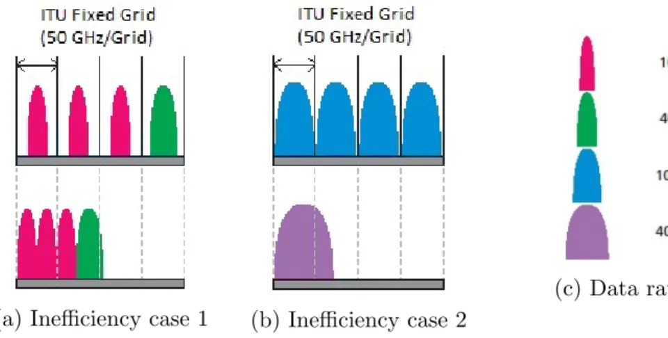
(a) Inefficiency case 1 (b) Inefficiency case 2

(c) Data rates

Figure 1.4: Illustration of WDM inefficiency cases

in the respective grid is directed to the same grid at the output port. Similarly, if there is a signal at an add port, it is directed to the output port’s respec-tive grid. OADMs are used for the construction of Wavelength Selecrespec-tive Switch (WSS) which is used for several purposes. Firstly, it adds signals generated by transponders to fibers connected to the WDM network. Secondly, it routes the signals in the intermediate nodes. Thirdly, when a signal reached to its destina-tion, WSS drops the signals to the optical receivers. Grooming the low traffics in WDM further increased system capacity. Developments in WDM created new demands for the optical networks and the traffic became more heterogeneous. To meet emerging heterogeneous demands, WDM was enhanced with transponders that support different modulation types to enable Mixed Line Rates (MLRs) on a single fiber.

In spite of the technological development in WDM network, the future demand needs more spectrally efficient approaches than WDM due to two main reasons. In the fixed grid structure of WDM, spectrum is wasted if required bandwidth is less or more than the fixed grid’s spectrum size [8]. These inefficiency cases are illustrated in Figure 1.4. In the first case, we have 4 transmissions with data rates {10,10,10 and 40} Gbps. The spectrum utilization of these data transmissions on WDM are illustrated in the upper part and the total needed bandwidth is illustrated in the lower part of Figure 1.4a. The bandwidth requirement for both 10 and 40 Gbps is less than the fixed grid size, thus the unused spectrum in the

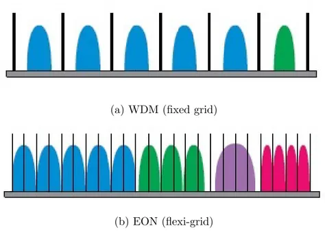
(a) WDM (fixed grid)

(b) EON (flexi-grid)

Figure 1.5: Illustration of Spectral occupancy by WDM and EON.

fixed grid is wasted. According to the illustration, half of the occupied spectrum in WDM is wasted. In the second case, we have only 400 Gbps whose bandwidth requirement is greater than fixed slice bandwidth. In this case, single subcarrier for 400 Gbps cannot be used due to the fixed grid structure. Thus, the demanded 400 Gbps is separated into 4 parallel 100 Gbps daha transmissions and 4 fixed slices are assigned to the demand. It is illustrated in Figure 1.4b that the wasted bandwidth is greater than the one actually needed. Thus, to increase the spectral efficiency of WDM networks, the rigid fixed grid structure must be replaced with a more flexible one to allocate the demanded bandwidth without wasting spectrum. Elastic Optical Network (EON) concept is proposed as a solution for this problem [9].

In EON, optical spectrum of links is divided into small slices of 6.25 GHz or 12.5 GHz [10] and a number of them can be allocated contiguously to cover a transmission’s requested subcarrier(s)’ total bandwidth. This structure is called flexi-grid, which is illustrated in Figure 1.5b. Black lines represents the slice

boundaries and the subcarriers with the same color belongs to the same super-channel which is a collection of subcarriers belonging to the same traffic demand. When the same bandwidth request is allocated with WDM as illustrated in Fig-ure 1.5a, only the half of the requests can be supported on the same amount of the spectrum. Thus, the flexi-grid structure of EON reduces the amount of bandwidth wasted in WDM network and increases the capacity utilization of the optical networks. To allocate a collection of slices for a demand and perform the modulation that fits to that bandwidth, the WSS component of WDM networks are replaced with Spectrum Selective Switches (SSS) and the transponders are replaced with Bandwidth Variable Transponders (BVTs) [11]. In this thesis, the spectrum size of a slice is used as 12.5 GHz.

In addition to the spectral efficiency, optical reach of the transmitted signal is another important parameter. In optical networks, the optical signal to noise ratio (OSNR) of the propagating signal decreases due to physical degradation from various different noise sources like intra-crosstalk, linear impairments and non-linear fiber effects [12]. The impairments cause stronger degradation as more bits are transmitted per a Hz of bandwidth [13]. To successfully transmit data, a sufficient quality of transmission (QoT) must be satisfied on the receiver side. The longest distance at which QoT (e.g., bit error rate) is satisfied, is called the maximum optical reach. To perform successful transmissions on a network, optical - electronic - optical (O/E/O) - based 3R (reamplification, reshaping and retiming) regenerators are used to extend the optical reach.

Originally, optical networks were operated with 3R regenerators on each node [14], namely opaque networks. Constructing and operating such a network causes a heavy burden due to expensive and high power consuming 3R regenerators [14]. Advances in optical technology enabled much higher bandwidth transmission and much longer maximum optical reach on a single fiber. For example, development of wavelength division multiplexing (WDM) and more advanced fiber amplifiers showed the importance of transparency in optical networks [14]. Also, trans-mission techniques such as time frequency packing (TFP) enabled optical com-munication over distances as long as 5000 km [15]. With such developments, opaque networks started to be replaced by translucent EONs by operators to

reduce capital and operational expenditures [16]. Translucent EONs promise to reduce opaque network’s electronic processing overhead by efficient and sparse utilization of regenerator resources [17]. Due to removal of 3R regenerators from some nodes, accumulated physical impairments will limit the optical reach of the network [14]. Another important property of the regenerators is their capability of changing the AMC profile already assigned to a transmission. Thus, the op-timum selection of minimum number of regenerator nodes in EONs becomes an important problem to both reduce capital and operational costs of regenerators and to use spectrum more efficiently with the reduced regenerator count.

In addition to the contiguity constraint of the slices assigned to the same superchannel in EON, the continuity of the assigned bandwidth throughout the optical light path is known to be another important concern [18]. In other words, the slices that are assigned to the segments, which are formed by the partitioning of a path with the regenerator nodes, must be same for all links of the segment. As a result, optimum selection of minimum number of regenerator nodes problem becomes harder with continuity constraint. However, developments in photonic device technology help reduce the limitation from this constraint. Nonlinear Optical Crystals (NOCs) are all optical components that can shift the frequency content of a signal on the optical spectrum [19]. Using these component, the slices assigned to a light path can be changed in the non-regenerator nodes in such a way that no overlap occurs between the slices of different light paths. NOCs are not as costly as 3R regenerators, thus, we assume that the non-regenerator nodes are placed with sufficient number of NOCs, and that we are not limited by the continuity constraint in the regenerator placement problem.

In this thesis, we focused on jointly selecting the AMC profile, routing and placement of the nodes performing 3R regeneration in EONs. Given a network topology, the purpose is to propose an offline regenerator placement with the objective of minimizing the number of nodes performing regeneration. For a set of demands which consist of source and destination nodes and bit rates, an ILP model is prepared to perform routing and AMC profile assignment of each demand for a given regenerator placement. The constraints of the ILP model are satisfying all demands, assigning a path to each demand, ensuring the maximum optical

Figure 1.6: Tabu Search Algorithm Illsutration.

reach by selecting appropriate AMC profiles, assigning sufficient number of slices according to the demanded bit rate and selected AMC profile and avoiding the violation of the link capacities. The routing of the demands are selected among a candidate path set, which is prepared according to two different approaches. In the first approach, k shortest paths (KSP) are utilized for any given regenerator placement. In the second approach, the candidate paths are determined according to the given regenerator placement to increase the system performance with the same computational complexity of KSP. This approach is named as Regenerator Location Dependent Path Selection (RLDPS). When the ILP model is solved, total link utilization is returned as a cost value. Our primary goal is to minimize regenerator nodes. Therefore, the link utilization cost value is combined with the number of selected regenerator nodes in such a way that number of regenerator nodes is prioritized.

In order to find minimum node regenerator placement, the computed cost values are utilized. Calculation of cost for all of the RP combinations is not practical. Therefore, we used Tabu Search metaheuristic to find minimum cost regenerator placement in reasonable amount of time. The brief idea is that each transition from previous state to the next state will be stored in the tabu list

and avoided to happen again. In this way, Tabu Search algorithm avoids the local minimums. In Figure 1.6, an illustration of local minimum avoidance is presented. The label of the nodes encircled are also their cost. The numbers on the transitions between nodes are the order of them. The neighborhood definition is being the adjacent node. The algorithm starts with node 20 as the initial node. If only the minimum cost neighbor is selected in each iteration, the search will stuck at the local minimum, which is 20. By the utilization of Tabu Search, node 50 is selected instead of node 40 in transition #3, because transition from node 20 to 40 is already in the tabu list. After this step, the algorithm leads to global minimum.

Based on the same idea above, Tabu Search based regenerator placement al-gorithm (TSRPA) is proposed to find minimum cost RP among all possibilities. The resultant RPs for randomly generated demand sets are combined to propose an offline RP as the weight of each node to be elected as regenerator. The results show that selection of candidate paths using RLDPS reduces network utilization either by decreasing the number of regenerator nodes by up to 66,6% or decreasing link capacity utilization by up to 5.09% as compared to KSP. The regeneration weight distribution obtained with RLDPS is more concentrated on specific nodes compared to KSP’s results and the results of the algorithms NSF, CNF and DA which are based on the topological properties of the nodes. As a result, RLDPS can route various sets of demand requests using smaller number of regenerator nodes compared to KSP. Thus, capital expenditures(CAPEX) of the network is reduced by RLDPS.

The remainder of the thesis is organized as follows. In Chapter 2, a literature survey on regenerator placement in translucent optical networks is provided. In Chapter 3, the iterative and modularized TSRPA is described and two candidate path selection algorithms, KSP and RLDPS, are explained. The performance of TSRPA with KSP and RLDPS are compared to show the importance of candidate path selection based on the regenerator locations in Chapter 4. Also, offline RP algorithms in the literature are compared with the proposed method in Chapter 4. Finally, the thesis will be concluded in Chapter 5.

Chapter 2

Literature Review

In this chapter, regenerator placement problem in translucent optical networks is introduced. Then, previous works done in this field of study are presented. Finally, the contribution of the thesis is described.

2.1

Regenerator Placement in Translucent

Op-tical Networks

In opaque networks, all nodes are placed with regenerators. Constraints like reachability or spectrum contiguity are not considered as a limiting factor. The drawback of opaque networks is their high capital and operation cost due to having high number of 3R regenerators. In translucent optical networks, the regenerators are sparsely placed on the nodes. In addition to reducing network cost dramatically, they can still perform very close to fully opaque networks [20]. Therefore, the objective of regenerator placement in translucent optical networks is to minimize the number of utilized regenerators.

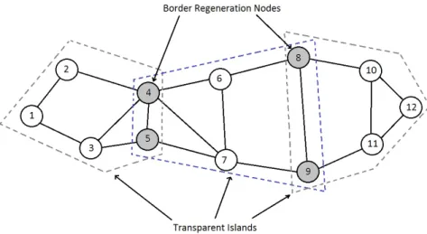
The translucent optical networks can be separated into 3 classes [21]. The first class is forming translucent optical networks with transparent islands. The

Figure 2.1: Illustration of transparent islands.

main idea is separating the network into non intersecting islands as illustrated in Figure 2.1 [22]. The nodes on the island borders are placed with regenerators and the transmissions crossing the border are regenerated if necessary due to the reachability constraint. Reducing the number of islands is the objective in this type of translucent networks, so that the number of regenerators nodes will be reduced. The second class of the transparent networks is to place regenerator nodes sparsely in the network [23]. The objective is to minimize the number of placed 3R regenerators on the network according to the given constraints like link capacity or reachability of the light paths. The third class is to form translucent optical networks using mixed regenerators which are named as 1R, 2R and 3R [14, 24] regenerators. The objective to reduce the number of utilized 3R regenerators which are more costly than others, by using 1R and 2R regenerators instead of 3R if possible. In this thesis, we constructed a translucent optical network with sparse placement of 3R regenerators.

The 3R regenerators in translucent networks can extend the optical reach of a transmission. It can change the modulation type and coding rate of the received signal and transmit it as an output. In this way, it can change the coded bit rate of the transmitted signal to adjust the level of increase in the optical reach. Due to changing modulation type and coding rate, the utilized optical bandwidth may change. Therefore, to utilize spectrum of the fiber effectively, 3R regenerators

can change the allocated spectrum for demands. These interesting properties of 3R regenerators can be leveraged to minimize their number in a fully operating network. The regenerator placement problem in translucent optical networks is aimed to minimized total number of 3R regenerators. It can be classified into two main approaches: In the first class, regenerator placement problem is solved without any traffic information, so the topological metrics are used. In the second class, regenerator placement is performed based on the traffic information.

2.2

Regenerator Placement without Traffic

In-formation

Most of the studies performed regenerator placement prior to applying their rout-ing and spectrum assignment algorithms. In the first class of regenerator place-ment, traffic information is not used.

Yang and Ramamurthy proposed Nodal Degree First (NDF) and Centered Node First (CNF) algorithms in [25]. NDF algorithm is based on the idea that the nodes that higher nodal degree than others are more likely to have regeneration demands. In the first step, the algorithm assigns the respective nodal degree values to the node. In the second step, the node with highest degree is selected as regenerator node. If there are multiple highest degree nodes, than one of the is chosen randomly. The selected node is removed from the list and the degree of the connected nodes are reduced by one. The step 2 is repeated until a specific number of regenerators are selected. CNF algorithm is based on the idea that the nodes located at the center of a network are more likely to have regeneration demand. The definition of being centered is the number of being visited by the shortest paths between all nodes in the network. Each node is assigned with a respective number and a set out of them is selected as it is done in NDF.

Aibin and Walkowiak proposed the Distance Adaptive (DA) Regenerator Lo-calication algorithm in [26]. For a given topology, each node is assigned with the

sum of all connected links’ lengths to them. Then, these values are divided with the sum of all link lengths. Finally, a set of regenerator units are distributed among the nodes according the resultant values of the nodes. After the selec-tion of regenerator nodes, the routes of the demands are selected among a set of candidate paths formed using 10 shortest paths.

2.3

Regenerator Placement with Traffic

Infor-mation

In the second class, traffic information is used to determine nodes that are likely to have regeneration demands.

Yang and Ramamurthy proposed Traffic Load Prediction based (TLP) and Signal quality prediction (SQP) based regenerator placement algorithms in [25]. TLP algorithm each node is assigned with a number that is initialized to zero. Then, a set randomly generated demands of a predicted traffic pattern are routed using a predefined wavelength routing algorithm. The numbers of the nodes that intersect with the routed demands are incremented by one. Finally, a set of nodes with highest values are selected as regenerators. SQP algorithm is similar to TLP. The only difference is instead of incrementing the values of nodes along the routes, only the value of nodes at which optical reach is exceed is incremented. The dependence to a wavelength routing algorithm is a drawback of these approaches. Shen et al. proposed a regenerator placement algorithm that is based on transition weights (TW) of the nodes in [27]. This approach is similar to CNF algorithm but the difference is about the increment values of the node. The traffic loads which are presented in Erlangs are added to the intersecting nodes. The regenerator nodes are selected according to the decreasing order of nodes’ resultant TW values.

Xie et al. focused on minimizing the number of regenerator sites for a set of demands with given routing in [28]. Cardinality of the nodes is the metric they

utilized in the regenerator placement problem. Briefly, if a node is in the middle of all routes of demand and the distances to both source and destination is equal to each other, then this node has the maximum cardinality. When the mixed line rates are considered, line rates are weighted to avoid cardinalty metric to always insist on lowest line rates.

Cerutti et al. addresses joint selection of code rate, the regenerator nodes, the spectrum allocation and routing in [2]. Initially a set of candidate regenerator nodes are selected. Then, with a set of pre computed candidate paths for each source and destination nodes, a feasibility metric is calculated for each candidate solution using proposed RSA-RA algorithm. According to the feasibility values of the candidate solutions, one of them is selected as a solution. New candidate solutions are generated from the selected one using a Genetic Algorithm meta heuristic approach, and feasibility values are calculated for them. This process is repeated for a certain amount of iteration number and a resultant solution is selected based on the feasibility values. Feasibility calculation can be modified to obtain minimum number of regenerator nodes or maximum spectral efficiency. In the algorithm above, the precomputed shortest paths for each source and destination node pair, are selected as 10 shortest paths.

Chaves et al. proposed two network traffic based algorithms called Most Used Regenerator Placement (MU-RP) and Most Simultaneously Used Regenerator Placement (MSU-RP) agorithms in [29]. According to the RWA and RA al-gorithms used in actual operation, MSU-RP algorithm places a number of re-generator units over the network. The maximum simultaneous utilization of a node is the metric for the regenerator placement. These algorithms depends on a preselected RWA and RA algorithms as it is done in TLP and SQP.

2.4

Contributions of the Thesis

Regenerator placement is generally performed prior to regenerator allocation and routing and spectrum assignment operations. Therefore, it is done as an offline

Figure 2.2: Flow Chart for Tabu Search based Regenerator Placement Algorithm (TSRPA).

operation. The previous works done in the literature mainly focused on topolog-ical properties if no traffic information is not available. Otherwise, for a given routing and spectrum assignment algorithm, the nodes at which regeneration is demanded are determined and regenerators are distributed among them. In most of these studies, the candidate paths for demands are selected as k shortest paths in the routing stage.

In this thesis, we propose an offline Tabu Search based Regenerator Place-ment Algorithm (TSRPA), that depends on no traffic information. The purpose is to minimize the number of nodes assigned with regenerators. The flow of the

TSRPA is illustrated in Figure 2.2. In this modularized and iterative approach, a tabu search algorithm is designed to find best regenerator placement according to their computed cost values. In the module 1, extend path sets between each source and destination node pairs are prepared according to the path length and hop count metrics using k shortest path algorithm. These paths are prepared by Module 1 at the beginning of the operation once and used throughout the optimization process. After the operation of Module 1 is completed, Module 2,3 and 4 iterates until the stopping criteria is satisfied. Module 2 is the main con-troller of the Tabu Search and it contains a tabu list to store previous transitions of regenerator placements in each iteration. It determines the best regenerator placements according to a cost value determined by Module 3 and 4. In each iteration, Module 2 prepare a set of candidate regenerator placements based on the decision made in the previous iteration. For each candidate, Module 3 and 4 are run to compute the cost value. Using these cost values and the tabu list content, a regenerator placement is selected among the candidates. In the module 4, an ILP model is prepared to solve routing and AMC profile assignment of all demands for the given regenerator placement. The routing of the each demand is selected among a set of candidate paths which are prepared by Module 3 ac-cording to two different approaches. The KSP approach simply selects k shortest paths computed in Module 1 based on the path distance metric. The RLDPS approach selects a subset of k shortest paths computed in Module 1 based on the hop count metric. The given regenerator placement plays the key role in the candidate path selection in RLDPS. Finally, the result of the ILP model is returned as a cost value to Module 2. This operation of Module 2,3 and 4 iterates for a predetermined number and when the limit is reached, the stopping criteria is satisfied. At this point, the regenerator placement with minimum cost value is determined as the solution. According to the numerical results, compared to the other offline regenerator placement algorithms that are based on topological properties like nodal degree or centrality of the nodes, the weight of the nodes to be selected as regenerator are more concentrated on specific nodes. Also, we showed that selection of candidate paths based on the regenerator placement with the RLDPS improves the performance of TSRPA by reducing the number of utilized regenerator nodes compared to the KSP.

The remaining of this thesis is organized as follows. In Chapter 3, the problem to be solved and the proposed solution TSRPA are described in details. The implementation of TSRPA, performed simulations’ settings and numerical re-sults are described along with their analysis in Chapter 4. Finally, the thesis is concluded in Chapter 5.

Chapter 3

Tabu Search Based Regenerator

Placement Algorithm

In this chapter, the iterative and modularized optimization approach for the joint selection of AMC profile, routing and placement of the nodes performing 3R re-generation in Elastic Optical Networks is presented. Initially the problem is stated and then the proposed Tabu Search based Regenerator Placement Algorithm is described.

3.1

Problem Overview

To propose a solution to the growing heterogeneous traffic demand, the devel-opment of EONs enabled the utilization of spectrum sources more flexibly. In addition to the flexible bandwidth utilization, the capabilities of the 3R regen-erators are increased compared to the ones used in WDM networks. According to the optical reach needed for a transmission, the 3R regenerators of EON can adjust the modulation and code rate without any spectrum limitation of fixed grid. Transmission techniques like TFP increased spectral efficiency and robust-ness against physical impairments [2]. Using this technique, the slices assigned

Table 3.1: Set of reachability and spectral efficiency required for 1Tb/s rate with different LDPC code rates [2].

AMC Code Reachability BW Subcarrier Slice

Profile Rate [km] [GHz] # #

1 9/10 3000 196 7 16

2 5/6 4000 224 8 18

3 3/4 5000 252 9 21

for each demand are utilized effectively with different modulation and coding rates, namely AMC profiles. In other words, each slice on a link can be assigned with an AMC profile, which corresponds to a spectral efficiency (b/s/slice) and reachability (km) metric [2]. In this thesis, 3 different code rate options presented in Table 3.1 are used as AMC profiles.

We have subcarriers with fixed data rate and the information rate can be changed using the code rates. Therefore, the number of utilized subcarriers are determined according to the selected coding rate and demanded bit rate. A col-lection of subcarriers assigned for a transmission is called a super-channel. Once the minimum sufficient subcarrier number is determined, slices are allocated to cover the super-channel bandwidth. In Table 3.1, the effect of LDPC code rate on the maximum optical reach and the corresponding spectral occupancy is illus-trated. Therefore, utilization of optical spectrum can be optimized by selecting the locations of 3R regenerators, the paths assigned to the demands and mini-mum required spectrum according to the selected AMC profiles to the segments. As a result, introduction of flexible spectrum assignment concept increased the complexity of the regenerator placement problem.

The problem can be modeled as a single optimization task. This approach can be used for small networks but, as the number of nodes increases, the effort required to solve the problem in single optimization step will increase exponen-tially. The studies in literature mainly focuses on two ideas. In the first one, if no traffic information is provided, selection of regenerator placement is based on nodes’ topological properties, such as nodal degree or centrality. In the second

one, according to the given traffic information, a set of demands are routed by a given routing and wavelength or spectrum assignment algorithm and regenerators are placed to the nodes where they are needed. In the routing stage, a set of k shortest paths are selected as candidate paths. In these approaches, the regen-erator placement is a decision that is made out of candidate paths. However, the selection of candidate paths are performed without taking the regenerator locations into consideration. Also, depending on a traffic information in the se-lection of regenerator placement will make the usefulness of the result specific to the given traffic trend. Therefore, selection of a regenerator placement without a given traffic information becomes an important problem.

In the thesis, we propose to solve this problem with an iterative and modular-ized approach in order to provide an offline regenerator placement for a topology. Given a regenerator placement, we prepared an ILP model to solve routing and AMC profile selection for a set of demands on a topology and the total link uti-lization along with number of utilized regenerator nodes are provided as a single cost value. In the model, each demand is assigned with a set of candidate paths and the model chooses one of them as the path of the demand. We propose a Regenerator Location Dependent Path Selection (RLDPS) algorithm to assess the importance of taking regenerator node locations in the candidate path selec-tion process, instead of simply utilizing k shortest paths. The purpose is to find the minimum cost regenerator placement. Instead of computing cost values of all possibilities, a Tabu Search metaheuristic is utilized to find minimum cost. In each iteration of the search, cost values are prepared for a set of candidate regenerator placements according to the result of routing and AMC profile selec-tion performed by the ILP model. A regenerator placement is selected among the candidates according to the Tabu Search criteria and the same process is repeated for a specific iteration number. The minimum cost regenerator placement that is found throughout the search is provided as output. The iterative algorithm is run for several randomly generated traffic loads and the results of them are combined as an offline regenerator placement.

3.2

Problem Definition

Regenerator Placement in Elastic Optical Networks with AMC can be explained as follows:

Given the topology information (nodes, links, link capacities and set of AMC profiles) and the demand set (source - destination nodes and demanded bit rates), find the nodes to be placed with regenerators such that;

• Primarily, the number of regenerator nodes is minimized.

• Secondarily, total utilized link capacity is minimized based on the selected regenerator locations.

• All requested demands are satisfied.

• Each demand is assigned a path in the network.

• Appropriate AMC profile(s) are selected for each demand such that maximum reach constraint is satisfied and sufficient number of slices are allocated. • Link capacities are not violated.

In the following section, the Tabu Search based Regenerator Placement algo-rithm, that is prepared to solve the problem with the given constraints above, is described in details.

3.3

Tabu Search based Regenerator Placement

Algorithm

The basic principle of Tabu Search (TS) is to avoid an algorithm stuck at a local minima by preventing repeating patterns, thus the global optimum can be found. TS utilizes a memory called Tabu List (TL) to store improving moves.

Non-improving moves in the following steps of the search are avoided using TL. The main process of TS can be divided into 4 steps [30]. In the step 1, current solution is initiated. In the step 2, a set of candidate moves are prepared. In the step 3, the most suitable candidate is selected as the current solution. TL content and objective of the search are the suitability constraints. In the fourth step, if stopping criteria is reached, the TS will be terminated. Otherwise, TL is updated and gone to step 2. A stopping criteria can be iterating for a predetermined number in total or since the detection of the last best solution.

In our proposed solution, for a predefined regenerator placement (RP), an integer linear programming (ILP) model is developed to solve routing of demands with a set of candidate paths. The ILP model provides a cost value as output. TSRPA is designed to find the minimum cost RP among the all possibilities. The inputs provided to the system are demand set (source-destination nodes and bit rates), topology information and AMC profiles. The parameters are Iteration Number (ITER NUM), Tabu List Size(TLS) and the Candidate Path Selection algorithm. Finally, a resultant RP with minimum cost and the routing of the demands are provided as the output of TSRPA.

The flow of the proposed solution is illustrated in Figure 2.2. Module 2 (Main Controller of TSRPA) manages the TS operation for TSRPA. In each iteration of the search, a new RP is selected amongst the candidates which are determined according to the current RP. Selection operation is based on the candidates’ cost values computed by Module 4 (Routing of Demands). For a given RP, a demand is routed acccording to a set candidate paths which are prepared by Module 3 (Candidate Path Set Selection). They are selected amongst a precomputed path set which are prepared by Module 1 (Extended Path Set Selection). Two different algorithms, named as k shortest path (KSP) and regenerator location dependent path selection (RLDPS), are used for candidate path selection. RLDPS and KSP algorithms are compared to assess the effect of RP based candidate path selection on RPP.

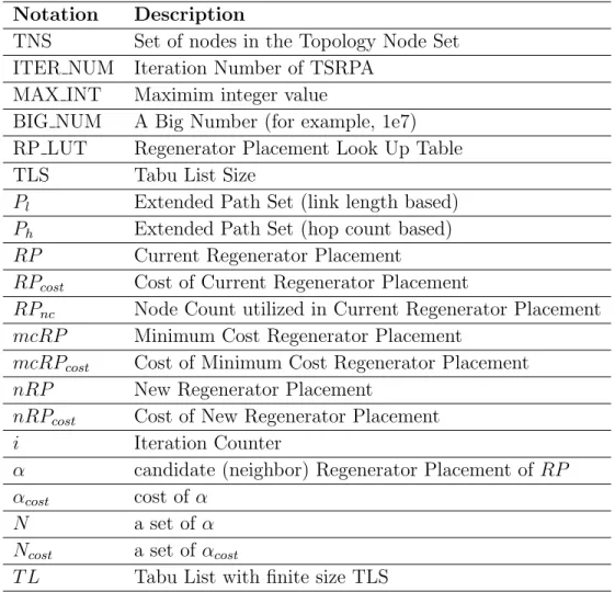
In the following subsections, details of these modules are explained. Notations used in these subsections are described in Table 3.2.

Table 3.2: Used Notations. Notation Description

TNS Set of nodes in the Topology Node Set ITER NUM Iteration Number of TSRPA

MAX INT Maximim integer value

BIG NUM A Big Number (for example, 1e7) RP LUT Regenerator Placement Look Up Table TLS Tabu List Size

Pl Extended Path Set (link length based)

Ph Extended Path Set (hop count based)

RP Current Regenerator Placement

RPcost Cost of Current Regenerator Placement

RPnc Node Count utilized in Current Regenerator Placement

mcRP Minimum Cost Regenerator Placement

mcRPcost Cost of Minimum Cost Regenerator Placement

nRP New Regenerator Placement

nRPcost Cost of New Regenerator Placement

i Iteration Counter

α candidate (neighbor) Regenerator Placement of RP αcost cost of α

N a set of α

Ncost a set of αcost

3.3.1

Module 1: Extended Path Set Selection

In Module 1, k shortest paths are calculated for each source - destination pair as extended set of paths (Pl and Ph) to be considered during optimization. The

Yen’s k shortest path algorithm [31] is used for this purpose. We use two different metrics for the candidate path selection algorithm: link length and hop count. The calculation process is performed once and used throughout the optimization process.

3.3.2

Module 2: Main Controller of TSRPA

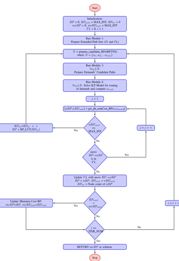
Module 2 is the main controller of TSRPA. For the given Topology Node Set (TNS), Tabu List Size (TLS) and Iteration Number (ITER NUM), it manages other Modules and leverages their outputs to find the mcRP by assessing the candidate RP s according to a TS operation. A finite memory TL is used and search is iterated for fixed ITER NUM. The operation of Module 2 is illustrated as a flow diagram in Figure 3.1. Briefly, operation starts with initialization of flow variables and Module 1’s extended path set calculation. Following the ini-tialization, the iterative operation starts.

At first, candidate RPs, represented as N , are prepared by using function prepare candidate RPs(RP,TNS). The details of this function is described in Subsection 3.3.2.1. For each element of N , Module 3 and 4 are run to select candidate paths for demands and then solve routing to obtain a cost value for each candidate RP respectively. Secondly, if minimum cost RP of N is infeasible (having cost value equal to MAX INT), then all element of N is infeasible. This case is observed at the beginning of TS due to initializing the solution RP as ∅. During this transient state, TSRPA is provided with predetermined regenerator placements from RP LUT memory. Thirdly, if minimum cost candidate of N is feasible (having cost NOT equal to MAX INT), the suitable candidate among N is selected as nRP and T L is updated with the move RP →nRP . Finally, if the nRP ’s cost is less than the mcRP , then it is also updated.

Start Initialization:

RP= ∅, RPcost= MAX INT, RPnc= 0

mcRP= ∅, mcRPcost= MAX INT

T L= ∅, i = 1 Run Module 1: Prepare Extended Path Sets (Pland Ph)

N= prepare candidate RPs(RP,TNS) where N = {α1, α2, ...α|N|}

Run Module 3: ∀αj∈N,

Prepare Demands’ Candidate Paths Run Module 4: ∀αj∈N, Solve ILP Model for routing

of demands and compute αcost

j= 1

[nRP ,nRPcost] = get jth minCost RP(α,αcost,j)

RPnc=RPnc+ + RP= RP LUT(RPnc) nRPcost == MAX INT j= j + + move RP→nRP is in T L

Update T L with move RP →nRP RP= nRP , RPcost= nRPcost

RPnc= Node count of nRP

Update Minimim Cost RP: mcRP=RP , mcRPcost=RPcost RPcost < mcRPcost i= i + + i== ITER NUM RETURN mcRP as solution. Stop No Yes No Yes No Yes No Yes

TSRPA iterates for ITER NUM cycles with a determined memory TLS and returns a RP. Since ∅ is selected as initial solution for TS, the consistency of the resultant RP depends on the selected ITER NUM and TLS. Therefore, TSRPA is run for several ITER NUM and TLS values to be sure about the consistency of the results.

3.3.2.1 prepare candidate RPs(RP,TNS)

The function prepares a set of candidate (neighbor) RPs, N , based on the given RP and TNS. We define 2 set, RP node set (RP N S) and complement of it, RP N Sc_{, such that RP N SS RP N S}c_{= T N S and RP N ST RP N S}c _{= ∅. Using}

RP N S and RP N Sc, we form the sets Nr, Na and Ns, such that;

• Nr is formed by removing a node from RP N S, so Nr consists of |RP N S|

elements.

• Na is formed by adding a node from RP N Sc to RP N S, so Na consists of

|RP N Sc_{| elements.}

• Ns is formed by removing a node from RP N S and adding a node from

RP N Sc to RP N S at the same time (switching nodes), so Ns consists of

|RP N S| ∗ |RP N Sc_{| elements.}

Finally, the set candidate (neighbor) RPs is formed as N = NrS NaS Ns.

3.3.3

Module 3: Candidate Path Set Selection

In Module 3, a candidate path set is prepared for each demand according to the selected candidate path selection algorithm (KSP or RLDPS). The extended

Figure 3.2: Illustration of penalty concept for segments and paths

paths sets, generated by Module 1 (Pl and Ph) are used for this purpose. KSP

algorithm performs selection based on the link length metric. Thus, KSP selects first k paths from Pl as candidate paths. Assignment of shortest path as routing

will be the best option in the perspective of a demand. However, when the reach-ability and link capacity constraints are taken into consideration, the shortest path might not be a good choice for routing of the demand. For example, if non of its nodes is a regenerator node and its total length is longer than maximum optical reach, then such a candidate path cannot be used as a solution. In this case, a longer path with a regenerator placed on it will be a better option. Thus, RP is an important parameter in the candidate path selection which is used to find mcRP .

Based on this motivation, we propose the RLDPS algorithm. Hop length met-ric is used as the primary criteria for RLDPS, so candidate paths are selected from Ph. Paths with equal number of hops are differentiated from each other

by a regenerator location based penalty metric. Regenerators divide paths into segments as illustrated in Figure 3.3. Each segment is assigned with an AMC profile related to its length. For example, as the segment length increases, band-width utilization increases due to the decreased code rate according to the AMC profiles defined in Table 3.1. Hence, we used the reachability of the AMC profiles as the penalty metric. If a segment’s length is less than the maximum AMC reachability, then penalties of 0, 1 or 2 are given for the selection of AMC profiles 1, 2 or 3 respectively. Otherwise, penalty of 3 is given to indicate the segment as useless. The penalty of the path is assigned as the maximum of its segments’

penalties and the paths with penalty 3 are eliminated. In Figure 3.2, we have a path divided into 2 segments by a regenerator node. The circles with S and D letters represents the source and destination nodes respectively. The square with an R letter is the regenerator node and the empty circles are the intermediate nodes. 2000 and 4500 km are the lengths of the segments. Therefore, the penal-ties assigned to them are 0 and 2 respectively. The penalty of the path is the maximum of segments’ penalties, which is 2. Finally, RLDPS sorts the remaining paths of Ph in the decreasing priority of minimum hop length, penalty and path

length. A specified number of sorted paths are selected as candidate paths.

3.3.4

Module 4: Routing of Demands

In Module 4, ILP model is formulated to optimally select one of candidate paths for each demand as its route and to assign AMC profiles to the selected path’s segments. The given RP will (possibly) divide these candidate paths into seg-ments and they will utilize slices on the links based on the assigned AMC profile according to their distance. The objective of the model is to minimize total slice utilization based on the Demand, Reachability and Link Capacity constraints. A cost value is returned as output. If a feasible solution is found, the cost value is set to summation of (BIG NUM * RPnc) and total number of slices utilized

on links. The purpose of this summation is to prioritize the selected number of regenerators over utilized link capacity. Otherwise, MAX INT is returned as output. TS process is iterated using these cost values. The details of the ILP model are explained in the following Section 3.4.

3.4

ILP Model for Routing and AMC Profile

Selection

In this section, the formulation of the ILP model for routing and AMC profile assignment for a given regenerator placement is described in details.

Figure 3.3: Illustration of relation between path, segment and link

3.4.1

Subscripts

The subscripts used in the formulation stand for the following words.

• i : demand • k : AMC profile • p : path

• r : segment • l : link

In the Figure 3.3, the relation between path, segment and link is illustrated. The meaning of the figure’s components are same as the ones in the Figure 3.2.

3.4.2

Inputs of the Model

Di : Demanded bit rate for demand i

Mk : Reachability value of the k’th AMC profile.

Sk : Spectral Efficiency value of the k’th AMC profile.

The symbol δiprl represents the selected candidate paths, which are prepared

in the Module 3, as follows.

δiprl=

 



1, if link l is on the segment r along the path p for demand i 0, otherwise

Cl : # of slices for link l. In other words, the capacity of link l is Cl. The

maximum of these capacities is C = max(Cl).

Al : length of link l in km.

All of these capacities are adjustable in our model.

3.4.3

Decision Variables

The decision variables of the model are described in this subsection.

yip =

 



1, if path p is selected for demand i 0, otherwise

nipr ∈ [0, C]: # of slices on segment r along path p for demand i.

ziprk =

 



1, if profile k is chosen on the segment r along path p for demand i 0, otherwise

When the ILP model is solved, the yipwill represent the selected candidate path

and the respective number of slices assigned to the segments of the selected path are represented by nipr for each demand. The total link utilization is determined

by the nipr values.

3.4.4

Constraints

The constraints of the ILP model are described in this subsection.

Constraint 1: For each demand, select only one path out of the candidate paths.

∀i :

X

p

yip = 1

Constraint 2: For each demand, select only one AMC profile for each segment of the selected path.

∀i, ∀p, ∀r:

X

k

ziprk = yip

Constraint 3 - Demand Constraint: For each demand’s selected path’s seg-ments, the assigned number of slices must be greater than or equal to the required number of slices for the demanded bit rate.

∀i, ∀p, ∀r :

X

k

Skziprknipr ≥ Diyip

ziprk and nipr. To linearize this constraint, we replaced the multiplication ziprknipr

with a new decision variable named as uiprk ∈ [0, C] such that. Thus, the

con-straint 3 becomes a linear concon-straint as follows:

∀i, ∀p, ∀r, ∀k: uiprk ≤ Cziprk

∀i, ∀p, ∀r, ∀k : uiprk ≤ nipr

∀i, ∀p, ∀r, ∀k : uiprk ≥ nipr− C(1 − ziprk)

∀i, ∀p, ∀r :

X

k

Skuiprk ≥ Diyip

Constraint 4 - Reachability Constraint: For each demand’s selected path’s segments, the reachability of the assigned AMC profile must be greater than or equal to the corresponding segment’s distance.

∀i, ∀p, ∀r : X l yipδiprlAl ≤ X k ziprkMk

Constraint 5 - Link Capacity Constraint: For each link, sum of all de-mands’ selected path’s corresponding segment’s number of assigned slices must be less than or equal to the link capacity.

∀l: X i X p X r niprδiprl≤ Cl

The objective of the ILP model is to minimize total utilized link capacity, which can be expressed as follows:

minX l X i X p X r niprδiprl

Finally, the total utilized link capacity is provided as an output of the ILP model. In the TSRPA, it is used to determined the minimum cost regenerator placement.

In the following chapter, the implementation and simulation settings of the algorithm are described. Then, the performance of TSRPA with KSP and RLDPS candidate path selection algorihms are evaluated. Also, the nodes’ weights to be selected as regenerator are compared with other proposed algorithms.

Chapter 4

Numerical Results

In this chapter, implementation of TSRPA and the simulation settings are pre-sented at first. Then, the performance of TSRPA with RLDPS is evaluated and compared to the case for TSRPA with KSP. The purpose of the comparison is to understand the effect of candidate path selection according to the regenera-tor locations (instead of selecting fixed set of shortest paths for any regeneraregenera-tor placement) on the network resource utilization. Moreover, the distribution of regenerator placements with TSRPA are compared with NDF, DA and CNF al-gorithms in the literature.

4.1

Implementation

The proposed TSRPA is implemented in C++ and the ILP model is formulated and solved using GUROBI optimizer[1], using its C++ application programming interface (API). The implementation details are described in 3 parts: the basic input and output relations, the implementation of TSRPA and the improvements on the time consumption of the algorithm.

At first, the parameters, basic input and output relations of the implemented TSRPA are briefly introduced. We have parameters that adjust the functionality

of the implementation before and after the compilation of the code. By adjust-ing the parameters in the code, we can change the existence of the program’s printouts for debugging purposes, number of parallel utilized CPUs by the ILP model, the timeout limit for the ILP model, the type of candidate path selection algorithm (KSP or RLDPS) and the number of utilized candidate paths in the simulation. Also, there are parameters to export useful data such as the con-tent of precomputed shortest paths, as text files. These parameters in the code cannot change the functionality of the program after the compilation. The resul-tant executable file (EXE) that is generated according to the parameters in the code, is used to run simulations. Then, a text file (IN TXT) is prepared with the parameters that determines the functionality of the generated EXE at the run time. These parameters consist of the id number of selected topology, the initial regenerator placement, the list of tabu list sizes and iteration numbers for TSRPA, and the demanded list which consists of bit rates, source and destination nodes. Finally, another text file (OUT TXT) is provided as an output when the operation is completed. It contains selected regenerator placement, total elapsed time, link loads obtained with the resultant regenerator placement and a brief summary of the simulation parameters. These are the basic input and output relations of our program implemented for TSRPA.

Secondly, the implementation of TSRPA is briefly described. The object ori-ented structure of C++ is used to prepare manageable and readable code for our modularized and iterative approach presented in Figure 2.2. Module 1 is imple-mented as a class called Topology. An instance of this class is provided with an id number of a predefined network topology. According to the given topology id, the id numbers of the nodes at both ends of the links and the length metric of the links are stored as the topology content. If RLDPS is selected as candidate path selection algorithm, then the link length metric is set to 1 to compute minimum hop paths. Otherwise, it is set to the link lengths in km to find the shortest paths. Module 2 and the stopping criteria are implemented according to flow diagram presented in Figure 3.1 as the main function of EXE. Finally, Module 3 and 4 are implemented as a single class called as Gurobi Optimization Model. In each iteration of the TSRPA, an instance of this class is provided with the demand

Figure 4.1: Gurobi APIs [1].

list, the instance of Topology class and candidate regenerator placement. In the first stage, the δiprl, which is containing the candidate paths for each demand, is

prepared by an internal function implementing the Module 3. In the second stage, the ILP formulation is solved using the C++ API of the GUROBI optimizer[1]. As illustrated in Figure 4.1, there are many other APIs supported by Gurobi and they share the common features like providing access to Gurobi Attributes in-terfaces and parameter sets. Using these APIs, an optimization model is defined in Gurobi with its decision variables, constraints and objective function. After the preparation of the model, it is solved according to the Gurobi parameters such as maximum number of threads and the timeout limit. The results of the optimization are returned as the values of the decision variables. Necessary data such as total link utilization is returned to the main function.

Optimization itself is a time consuming process and when it is performed iter-atively, total elapsed time for the whole process becomes an important concern. Therefore, we improved the time consumption with several techniques. The first one is using C++ as the programming language to increase the computation speed of operations except the optimization process. The second one is, comput-ing the cost of all scomput-ingle and double node regenerator placement combinations before running the TSRPA to see whether any one of them is feasible or not. Our

primary goal is to reduce the number of regenerator nodes, therefore if the solu-tion is a single or double node, then time can be saved with a brute force search among these combinations instead of running the TSRPA. In the third one, the time consumption of TSRPA is reduced by storing the computed optimization cost values of regenerator placements to reuse them when needed in the Tabu Search because the cost value is deterministic for a given regenerator placement in our model. When the tabu search found the global minimum, the candidate regenerator placements in the following iterations of the algorithm selected simi-larly. In other words, due to the limited tabu memory size of the TSRPA, we can observe repeating candidate regenerator placements in the case of no improve-ments throughout the search. In such cases, utilization of previous results saves huge amount of time.

In the next section, the settings of the simulations are briefly described.

4.2

Settings

The 14 node NSFNET and 24 node US National Network (USANET) topologies are used for performance evaluation. They are presented in Figure 4.2 with node labels and link lengths in km. Link capacities are set to 100 slices for both topologies. The static traffic info is prepared as 15 demand sets. Thus, we performed 15 different simulations for both of the topologies. Number of optical demands are distributed evenly as 70, 80, 90 for NSFNET and 80, 90 and 100 for USANET. Demands are full duplex and each routed direction follows the same path. There can be only one demand defined between two nodes. The bit rate for each optical connection request is selected uniformly from the data rate set {100 Gbps, 400 Gbps, 1 Tbps}. The AMC profiles in Table 3.1 are used in the simulation. The slice utilization of AMC profiles for a given demanded bit rate are presented in Table 4.1. To determine the sufficient number of candidate paths, we performed experiments with 3, 5, 7 and 9 candidate paths. According to experimental results, selection of 5 paths as candidate are observed to be enough. Due to utilizing an iterative approach, we set 1000 seconds of timeout

(a) 14-Node NSFNET.

(b) 24-Node US National Network.

Figure 4.3: Flow formulation of a reduced demand set.

for optimization of the ILP model. Finally, to obtain a consistent result, TSRPA is run for cases ITER NUM = {20,100,1000} and TLS = {5,20,100} to have a reliable resultant RP. The simulations are performed in the following order of ITER NUM and TLS combinations.

• 1st _{: ITER NUM = 20 , TLS = 5.} • 2nd _{: ITER NUM = 20 , TLS = 20.} • 3rd _{: ITER NUM = 20 , TLS = 100.} • 4th _{: ITER NUM = 100 , TLS = 5.} • 5th _{: ITER NUM = 100 , TLS = 20.} • 6th _{: ITER NUM = 100 , TLS = 100.} • 7th _{: ITER NUM = 1000 , TLS = 5.} • 8th _{: ITER NUM = 1000 , TLS = 20.} • 9th _{: ITER NUM = 1000 , TLS = 100.}

Table 4.1: Number of slices needed for a Demanded bit rate using an AMC profile Demanded Bit Rate

(Gbps) 100 400 1000 AMC Profile ID 1 2 7 16 2 2 7 18 3 3 9 21

Due to the slice limitation on the links, the existence of a solution for a given demand set must be validated at first. Regeneration at every node is the most optimistic regenerator placement. Therefore, if no feasible solution exists for the this case, then we can say that there exists no solution for this demand set. For this purpose, a flow formulation is prepared to route all demands on the selected topology as if all the nodes are placed with regenerators. The link capacity constraint is applied and each demand is routed with no loop. For example, flow formulation is applied to randomly generate demand sets and the total link utilization is illustrated on network topology. For some cases, all of the demands could not be routed. In these case, a demand is taken out from the set and the flow formulation is applied again. We repeated this process until we obtain a feasible routing. In one of our trials with 90 demands at the beginning, we obtained a feasible solution with 84 demands as illustrated in Figure 4.3. In the topology, the links are labeled with numbers in braces with red color. In the results of the flow formulation with reduced demand set, we have links {12, 13, 15, 16 and 25} highly congested. The links {12, 13, 15 and 16} form a boundary between two sides of the topology, so they form a bottleneck in the topology. In this situation, new demands cannot be supported by this topology. Thus, there is no solution for this demand set. Flow formulation showed us that if the demand number goes beyond 100 for USANET topology, high congestion in the middle part of the network caused most of the generated demands be unsolvable due to our 100 slice limitation on a link. Thus, we selected 80, 90 and 100 as our demand set number for USANET topology for the given link capacity constraint.