Entanglement in local systems

a dissertation submitted to

the department of physics

and the institute of engineering and science

of bilkent university

in partial fulfillment of the requirements

for the degree of

doctor of philosophy

By

Sinem Binicio˘glu C

¸ etiner

January, 2008

Prof. Alexander S. Shumovsky (Late) Prof. Atilla Er¸celebi (Supervisor)

I certify that I have read this thesis and that in my opinion it is fully adequate, in scope and in quality, as a dissertation for the degree of doctor of philosophy.

Assist. Prof. ¨Ozg¨ur Oktel

I certify that I have read this thesis and that in my opinion it is fully adequate, in scope and in quality, as a dissertation for the degree of doctor of philosophy.

Prof. Alexander Klyachko ii

Assoc. Prof. Ulrike Salzner

I certify that I have read this thesis and that in my opinion it is fully adequate, in scope and in quality, as a dissertation for the degree of doctor of philosophy.

Prof. Yi˘git G¨und¨u¸c

Approved for the Institute of Engineering and Science:

Prof. Dr. Mehmet B. Baray Director of the Institute

Sinem Binicio˘glu C¸ etiner Ph. D.in Physics

Supervisors: Prof. Alexander S. Shumovsky (Late) Prof. Atilla Er¸celebi and

Assist. Prof. ¨Ozg¨ur Oktel January, 2008

In this study, we first discuss entanglement measures and we introduce a way to construct generic entangled states of an n-level quantum system.

Then we discuss entanglement as a local object. Particularly we use a spin qutrit, and investigate whether an entangled spin qutrit obeys entanglement cri-teria or not. While doing this, we also discuss, which cricri-teria of entanglement are essential and which of them are not. We show the relation between quantum fluctuations and entanglement.

Lastly, we discuss Bell type inequalities and we show violation of a Bell type condition by a single particle entangled state.

Keywords: Quantum entanglement, entanglement measures, quantum informa-tion, foundations of quantum mechanics, entanglement and quantum nonlocality, Bell type inequalities.

YEREL SISTEMLERDE DOLAN˙IKL˙IK

Sinem Binicio˘glu C¸ etiner Fizik, Doktora

Tez Y¨oneticileri: Prof. Alexander S. Shumovsky (M¨uteveffa) Prof. Atilla Er¸celebi ve

Assist. Prof. ¨Ozg¨ur Oktel Ocak, 2008

Bu ¸calı¸smada, ¨oncelikle dolanıklı˘gın ¨ol¸c¨us¨u tartı¸sılmı¸s ve n-seviye bir kuvantum sisteminin genel dolanıklık hallerini kurmak i¸cin bir y¨ontem tanıtılmı¸stır.

Sonra dolanıklık yerel bir nesne olarak tartı¸sılmı¸stır. ¨Ozellikle bir spin ¨u¸c se-viyeli sistemi kullanılmı¸s ve dolanık bir spin ¨u¸c sese-viyeli sistemin dolanıklık kriter-lerine uyup uymadı˘gı ara¸stırılmı¸stır. Ayrıca bu yapılırken, dolanıklı˘gın hangi kriterlerinin gerekli olup hangilerinin gerekli olmadı˘gı tartı¸sılmı¸stır. Kuvantum dalgalanmaları ile dolanıklık arasındaki ili¸ski g¨osterilmi¸stir.

Son olarak, Bell tipi e¸sitsizlikleri tartı¸sılmı¸s ve Bell tipi bir ¸sartın, tek par¸cacık dolanık hali tarafından ihlal edildi˘gi g¨osterilmi¸stir.

Anahtar s¨ozc¨ukler : Kuvantum dolanıklık, dolanıklık ¨o¸c¨uleri, kuvantum enfor-masyon, kuvantum mekani˘ginin temelleri, dolanıklık ve kuvantum yerelsizli˘gi, Bell tipi esit¸sizlikler.

This thesis is a product of almost three years that I have spent with Prof. Shumovsky. Within these three years, he was an “advisor” to me not only with his knowledge but also with his attitude towards life.

The working group that I have been into for these years, had accomplished very good jobs, with Prof. Shumovsky’s unending enthusiasm, Prof. Klyachko’s creativity, M. Ali Can’s wisdom, and ¨Ozg¨ur C¸ akir’s ingenuity. I wish I could have spent more time with them.

In life, most of us eat, drink, sleep while dealing with daily troubles, just a few of us really live. Prof. Shumovsky lived a very beautiful life with his humor, knowledge, good manners, and joy of life. I will never forget this person who, by frequently advising me to “calm down”, had let me be able to pause sometimes in life and look around. It is a duty for me to express my gratitude to those people who made my life more meaningful, to my friends and to my family for their support and trust.

I also thank to the jury members Prof. Er¸celebi, Prof. Oktel, Prof. Salzner, and Prof. G¨und¨u¸c, who spent their time to evaluate my work.

With my wish of being worthy, this study is dedicated to the precious memory of Prof. Shumovsky.

1 Introduction 1

2 Generic Entanglement 4

2.1 Entanglement measures . . . 4

2.1.1 Information Entropy . . . 6

2.1.2 Concurrence . . . 7

2.1.3 Variance as a Measure of Entanglement . . . 10

2.2 Generic Entangled States . . . 17

2.2.1 SU(2) Phase States . . . 17

2.2.2 Generic Entanglement . . . 19

2.3 Summary . . . 22

3 Single Particle Entanglement 24 3.1 Entanglement and nonlocality . . . 24

3.2 SU(2) qutrit . . . 26

3.3 Entanglement and quantum fluctuations . . . 31 vii

3.3.1 The SU(2) coherent states are unentangled . . . 32

3.3.2 “Squeezed” spin states . . . 36

3.3.3 Spin coherence and “squeezing” . . . 38

3.4 Physical realizations of single spin-qutrit entanglement . . . 41

3.5 Summary . . . 46

4 Violation of Bell type condition without nonlocality 47 4.1 Introduction . . . 47 4.1.1 Bell’s inequality . . . 49 4.1.2 CHSH inequality . . . 51 4.2 Pentagram inequality . . . 53 4.3 Summary . . . 58 5 Conclusions 59 A Algebra of observables 62 B Density matrix 64 B.1 Reduced density matrix . . . 65

C Qubit 68 C.1 Symmetric two-qubit state . . . 70

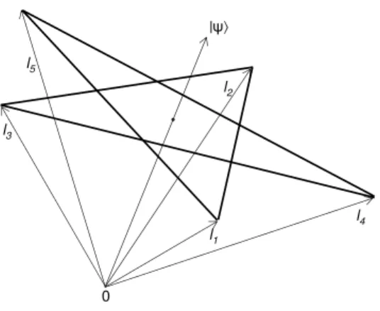
3. 1 Interaction between λ-type three-level atom and two cavity modes. 43 4. 1 Regular pentagram defined by cyclic quintuplet of unit vectors

`i ⊥ `i+1. State vector |ψi is directed along the symmetry axis of

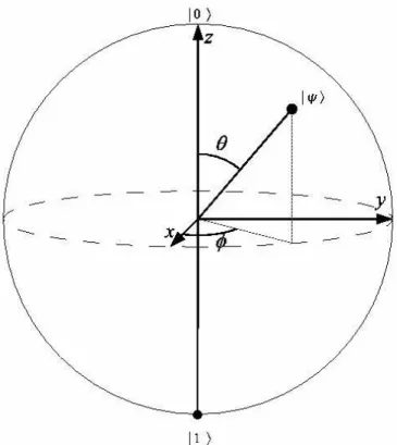
the pentagram. . . 55 3. 1 Bloch sphere. |0i and |1i states are represented by the points

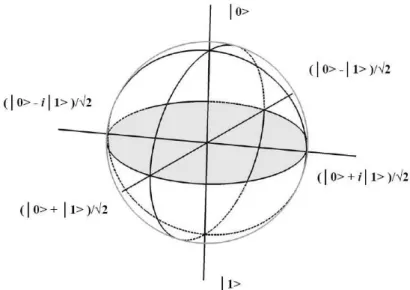
(0, 0, 1) and (0, 0, −1) on Bloch sphere respectively. . . . 70 3. 2 |0i (|1i) state, represents spin up (down) | ↑i (| ↓)i state for

spin−1/2 particle; ground (excited) level |ei (|gi) for two-level atom, and right (left) circularly polarized state |Ri(|Li) for po-larization of a photon. . . 71

Introduction

Quantum entanglement is a phenomenon which has no classical analog. Its prac-tical importance could not be understood for a long time. Recent developments of quantum information technologies have led to a number of successful and promis-ing realizations of protocols, based on the use of quantum entanglement. For example, quantum key distribution has recently become an industrial product [1].

Quantum information can be defined as a physical information held in the state of the quantum system. Quantum systems are described by quantum states, which are linear combinations (superposition states) of the eigenstates of the observables. If a measurement is done, the state will be randomly collapsed onto one of the eigentstates in the superposition . Superposition of multipartite states is connected with notion of entanglement. Entanglement arises due to nonclassical correlations in a quantum system. Once subsystems of a composite quantum system are interacted, their states may be superposed with one another, the systems may be “entangled”.

Development in quantum information science caused a great burst of activ-ity in the investigation of quantum entanglement. During the last decade, the applications of entanglement were discussed by a number of groups all around the world. With the aid of quantum information, we can perform certain tasks,

that are not possible classically. For example quantum computers (they can per-form some tasks which are difficult or impossible for classical computers) [2]; quantum cryptography (unconditionally secure transmission of information) [3]; dense coding [4], and teleportation [5] became possible with the use of quantum information.

Entanglement is widely considered as a property of nonlocal systems, this is also useful for communication purposes, where individual parties of the system are well separated. We proposed [6, 7] that, entanglement can also be considered as a property of local systems (as well). In some local systems, intrinsic degrees of freedom of a single particle can be entangled. We can easily see the entangle-ment of such a particle if it decays into two separated, entangled particles (e.g. biphoton). Our concern is, can we observe entanglement before the decay? In fact,we can observe violation of classical realism by such a state.

To make separate measurements on different degrees of freedom of a single particle is a hard task with the existing experimental techniques. However we can argue some principles of entanglement, which of them are essential and which of them are not. And we can check whether our proposition obeys to essential properties of entanglement or not.

Discussion of entanglement as a local object may not be useful for practical purposes (especially for communication purposes) for now, however it is very important for the understanding the physics behind entanglement. It may be useful in the future, especially for computation purposes.

While describing entanglement physically, we should also give a quantative description of it. A technique to quantify entanglement is proposed by our group [8, 9], this technique is based on specifying the quantum system by accessible observables, and it relates quantum fluctuations with entanglement.

The thesis is organized as follows:

In the second chapter; firstly we discuss some entanglement measures, and we introduce variance as a measure of entanglement. Then, an algebraic way to

construct generic entangled states of qunits based on the polar decomposition of the su(2) algebra is discussed. In particular, we show that these states can be defined as eigenstates of certain Hermitian operators.

In the third chapter; first we discuss the physical properties of entanglement. We discuss the entanglement of SU(2) qutrit and its correspondence with two-qubits. Then we show the relation between the quantum fluctuations and en-tanglement. Lastly we propose some physical systems to realize single particle entanglement.

In the fourth chapter, we discuss the Bell’s inequalities. Firstly, we recall Bell’s original inequality and CHSH (Clauser, Horne, Shimony, and Holt) in-equality. Then we introduce our “pentagram inequality”, and give violation of this inequality by a single qutrit state.

In appendices, we give deeper explanations of the notions that we used in our text.

Generic Entanglement

In this chapter we first summarize some techniques to measure entanglement and then introduce Generic Entangled States.

2.1

Entanglement measures

Entanglement was first introduced to quantum mechanics by Einstein to show the inconsistency in the statistical nature of the theory [10]. In the famous paper “Can Quantum-Mechanical Description of Physical Reality Be Considered Com-plete?” Einstein, Podolsky, and Rosen discussed the uncertainty principle. They considered two separate systems I and II, which interacted for a time but have no interaction after a while. By performing simultaneous measurements to each subsystem, they concluded that it is possible to predict physical quantities de-scribed by noncommuting operators. However according to quantum mechanics, if two operators are noncommuting, correlation type measurements are not pos-sible. Those discussions led to remarkable proposal of the states that manifest quantum nonlocality and to an attempt to adjust these spooky states with the “classical common sense” by means of the hidden variable modification of quan-tum mechanics. Nonlocality means that, if a measurement is done on one part of the separated quantum system, this measurement can also influence other parts,

due to nonclassical correlations between them. Hidden variable theories are based on two joint assumptions; existence of reality before observation (realism), and locality. Bell was not convinced with the hidden variables in quantum theory. He introduced his famous inequalities to show nonexistence of hidden classical variables in quantum mechanics [11].

Entanglement can be associated with nonclassical correlations in a quantum system. Detection and quantification of entanglement is important for both the-oretical and practical aspects. Although Bell’s inequalities were introduced to show nonexistence of hidden variables in quantum mechanics, they also served to detect the entanglement in a given quantum system.

Separability condition is another criterion for entanglement. Nonseperability can be related with nonlocality principle. For pure states by decomposing the states into Schmidt form [12] one can easily check the separability of the state. For mixed states, separability condition becomes harder, for them entanglement witnesses can be used as a criterion [13]. Although the separability criterion works well for bipartite systems, it has no meaning for single particle system. Also it does not work well for some three partite states (GHZ and W-states).

To give a quantitative measure of entanglement is harder then to give a qual-itative test. For this aim we need operations that can be applied to quantum system and that can create or increase only classical correlations (not quantum correlations). So entanglement cannot be created via such operations. If a number assigned to the state is not increasing under such operations it can be considered as an entanglement measure. Any scalar valued function that satisfies this cri-terion is called an entanglement monotone. The operations mentioned above are called local operations assisted by classical communications (LOCC )[14]. LOCC imply general local operations, and also allow for classical correlations between them. There is another class of operations called stochastic local operations as-sisted by classical communications (SLOCC ). SLOCC is more useful especially for multipartite states. [15, 16, 17].

SLOCC can be described as classification of entanglement, which is a coarse-grained classification of entanglement under LOCC [18].

Some important properties of entanglement monotone can be summarized as; it should be invariant under local unitary transformations, should be zero for a separable state, should take maximum value for Bell states, and should give asymptotic conversion rate from an arbitrary state to a standard Bell state.

Below some entanglement measures are summarized:

2.1.1

Information Entropy

Claude Shannon established some core results in classical information theory [19]. Shannon entropy quantifies the amount of uncertainty in the system (in other sense lack of knowledge). Let X be a discrete random variable taking a finite number of possible values x1, x2, · · ·, xn with probabilities p1, p2, · · ·, pn

(Pn

i=1pi = 1). Shannon entropy can be formulated as:

H(p1, p2, ..., pn) = − n

X

i=1

pilog2pi. (2. 1)

Entropy becomes maximum if we do not have any information about the outcomes of the measurement, i.e. they are all equally likely. For bipartite case binary entropy takes the form

H(p) = −p log₂p − (1 − p) log₂(1 − p) (2. 2) where p and 1 − p are the probabilities of the two outcomes.

In the case of quantum information, random variables become density matri-ces. Von Neumann entropy is the quantum counterpart of the classical Shannon entropy [20]:

S(ρ) = −T r(ρ log₂ρ) (2. 3)

In terms of the spectrum αi of the density matrix ρ we can convert equation to

the following:

S(ρ) = −Σiαilog2αi (2. 4)

Von Neumann entropy of a pure state is zero, whether it is entangled or not. For a completely mixed state ρ = I/n in n − dimensional system it takes maximum possible value S(ρ) = log₂n. But if we take the von Neumann entropy of the reduced density matrices we will get an entanglement monotone called entanglement of formation[21]:

E(ψ) = −T r(ρrlog ρr) (2. 5)

for a pure state and

E(ρ) = minΣpiE(ψi) (2. 6)

for a mixed state. It is not important which subsystem we are using. Even if their dimensions are different they have the same nonvanishing eigenvalues, and this is the part that is invariant under unitary transformations. Entanglement of formation takes the value zero for separable states. Let’s calculate it for Bell state:

ρ = |Ψ+

BellihΨ+Bell| =

        1 0 0 1 0 0 0 0 0 0 0 0 1 0 0 1         . (2. 7)

Partial traces become

ρ1 = ρ2 =   1/2 0 0 1/2   _{(2. 8)}

and entanglement of formation takes the maximum value (one) for the Bell state. It gives us the degree of quantum correlation in the system.

For mixed states, to find an analytic solution of entanglement of formation is very hard. But for two qubits, an analytic expression is introduced by Wootters [22, 23].

2.1.2

Concurrence

Wootters’s starting point was a useful fact about pure states of two qubits. If we define the orthonormal basis of the four dimensional Hilbert space of two qubits

in terms of Bell states with different phases (magic basis): |e1i = 1₂(|00i + |11i) |e2i = 1₂i(|00i − |11i) |e3i = 1₂i(|01i + |10i) |e4i = 1₂(|01i − |10i) (2. 9)

an entanglement monotone called concurrence of a pure state |ψi =P_iαi|eii can

be defined very simply [22]

C(ψ) = |X

i

α2

i|. (2. 10)

There is a strong relationship between concurrence and entanglement of forma-tion:

E(ψ) = H(1 2(1 +

√

1 − C2_{)) (2. 11)}

Hence, once we find concurrence we can easily calculate entanglement of formation for a pair of qubits. Concurrence can also be considered as a measure alone. An analytic expression of concurrence for mixed states is also present [23]. For this aim we should calculate spin-flip transformation of the density matrix

˜

ρ = (σy⊗ σy)ρ∗(σy ⊗ σy) (2. 12)

where the ρ and complex conjugation ρ∗ _{is taken in the standard basis}

|00i, |01i, |10i, |11i. In fact spin-flip transformation is just complex conjugation in the magic basis. Concurrence for any bipartite two level system can be formulated as following:

C(ρ) = max(0, λ1 − λ2− λ3− λ4) (2. 13)

where λi’s are square roots of the spectrum of the matrix ρ˜ρ, in decreasing order.

We can write a general two-qubit state as following

|ψi = a|00i + b|01i + c|10i + d|11i, (2. 14)

and concurrence for such a state becomes

There also exists an analytic measure of entanglement for three qubits. Three-qubit states may manifest entanglement of two different types. Namely, entan-glement caused by correlations of all three qubits and entanentan-glement due to cor-relation between pair of parts [15]. The three-qubit entanglement is measured by means of 3-tangle [17, 24], which for the general state

|ψi = 1 X k,`,m=0 ψk`m|k`mi, 1 X k,`,m=0 |ψk`m|2 = 1,

has the form

τ (ψ) = 4|ψ2

000ψ2111+ ψ2001ψ1102 + ψ2010ψ1012 + ψ2100ψ0112

−2(ψ000ψ001ψ110ψ111+ ψ000ψ010ψ101ψ111+ ψ000ψ100ψ011ψ111

+ψ001ψ010ψ101ψ110+ ψ001ψ100ψ011ψ110+ ψ010ψ100ψ011ψ101)

+4(ψ000ψ011ψ101ψ110+ ψ001ψ010ψ100ψ111)| (2. 16)

According to classification by Miyake [17], the following three states

|GHZi = √1

2(|000i + |111i), (2. 17)

|W i = √1

3(|011i + |101i + |110i), (2. 18) |Bii = √1

2(|011i + |101i) (2. 19)

are generic for the three SLOCC-nonequivalent classes in the eight-dimensional Hilbert space. The non-separable states from the GHZ class manifest only three-partite entanglement (3-tangle (2. 16) has nonzero values for the states from this class), while any pair of qubits is unentangled. The latter can be checked by reduction of the three-qubit density matrix ρGHZ = |GHZihGHZ| to the

two-qubit mixed state ρ0

GHZ = TrsingleρGHZ, where Trsingle denotes trace over one of

the parts, with the subsequent calculation of the concurrence, which in this case always has zero value.

In turn, the non-separable states from the W class always have zero 3-tangle and hence do not manifest three-partite entanglement, and any bipartite reduced state with the density matrix ρ0

W = Tr(|W ihW |) has nonzero concurrence and

Finally, the separable states from the Bi class are similar, in a sense, to the W states. Namely, they always have zero 3-tangle while manifest bipartite en-tanglement (for two given qubits only).

Thus, the nonseparability (separability) of the three-qubit states does not in-dicate identically the presence (absence) of entanglement and its type in contrast to the bipartite systems.

In the case of three-qubits, Von Neumann entropy does not work. Consider as an example the GHZ-type state of the form |Ψi = x|000i + y|111i, x2_{+ y}2 _{= 1.}

It is seen that 3-tangle (2. 16) τ (Ψ) = 4x2_y2 _{= 4x}2_{(1 − x}2_{), so that the state}

is entangled (in the three-part sector) for all x ∈ (0, 1). The reduced two-qubit density matrix for any pair of qubits has the form

ρR= x2|00ih00| + (1 − x2)|11ih11|

with the corresponding von Neumann entropy

H(ρR) = −x2log x2− (1 − x2) log(1 − x2).

Subsequent reduction of ρR to the single-qubit state

ρRR = x2|0ih0| + (1 − x2)|1ih1|

obviously leads to the same von Neumann entropy H(ρR) as ρR, although there

is no two-qubit entanglement in the state. Similar behavior, showing unfitness of the reduced state entropy as a general measure of entanglement, is manifested by the W and Bi states of three qubits as well.

There is a need of a measure of entanglement based on physical manifestations of entanglement in the process of measurement of quantum observables, which is related with total amount of quantum correlations in the given system.

2.1.3

Variance as a Measure of Entanglement

There is a certain interdependence between quantum correlations peculiar to entangled states and quantum uncertainties (fluctuations) of local observables

[8, 9, 25]. Consider as an illustrative example the measurement of spin projection onto the quantization axis in the two-qubit states |ψ00i = |00i and |ψCEi =

(|00i + |11i)/√2. For the correlation functions and variances (uncertainties), we get

hψ00|σzA; σBz|ψ00i = 0, V (σA,Bz ; ψ00) = 0,

hψCE|σzA; σBz|ψCEi = 1, V (σA,Bz ; ψCE) = 1.

Here σA

z, σBz denote the z-component of Pauli spin operator,

hψ|σA_{; σ}B_{|ψi = hψ|σ}A_σB_{|ψi − hψ|σ}A_|ψihψ|σB_|ψi

is the correlation function of local measurements, and V (σ; ψ) = hψ|σ2|ψi − hψ|σ|ψi2

is the variance of the observable σ in the state ψ. Thus, the correlation functions and variances have similar behavior for unentangled states like ψ00and entangled

states like ψCE.

The natural question now is how many physical observables should be mea-sured in order to conclude that a given state of a certain system is entangled [26]? This question has extremely high importance for understanding of physical essence of entanglement and its quantification. Besides that, this question has a quite practical meaning in connection with test of sources of entangled states [27].

In a recent approach [8, 28, 29] (for recent review, see Ref. [30]), it has been proposed to begin the analysis of entanglement with the choice of independent basic observables that can be associated with the orthogonal basis of a certain Lie algebra L. The corresponding Lie group G = exp(iL) defines the dynamic symmetry of the physical system under consideration.

It should be emphasized that the idea to specify a quantum system by ac-cessible observables is known for a long time (e.g., see [31]). Unfortunately, this principle idea is often set aside. As we show below, this principle plays extremely important role in description of quantum entanglement.

Within the approach of Refs. [8, 28, 29], the complete entanglement is inter-preted as manifestation of quantum uncertainties of all basic observables at their extreme. By complete entanglement we mean here the maximal entanglement that can be achieved by pure states.

Note that, for a given quantum system, it is enough to know the completely entangled states because all other entangled states can be generated from those states through the use of SLOCC [15, 16].

We will discuss the characteristic features of this approach, using a single qutrit (ternary quantum state) as an illustrative example of some considerable interest.

Qutrit is usually associated with ternary unit of quantum information [32]. In-structiveness of this example lies in the relativity of entanglement with respect to the choice of dynamic symmetry G of ternary quantum physical system. Namely, one can choose either G = SU(3) [33] or G0 _{= SU(2). Just the latter case of a}

single spin-1 system may manifest entanglement without division of the system into separated parts [6, 28, 34].

As mentioned, specifying a given quantum system, we should first choose the accessible independent physical observables associated with dynamic symmetry of the system.

For example, in the case of a qubit (spin 1/2) system, dynamic symmetry is given by the group SU(2). The orthogonal basis of the corresponding Lie algebra su(2) consists of three spin operators (Pauli matrices). Thus, a two-qubit system is characterized by the dynamic symmetry G = SU(2)×SU(2), which corresponds to the six basic observables (three Pauli matrices for each part). For the two-qubit pure state, the number of necessary measurements, providing information about entanglement carried by this state, is reduced to three [26] because of the local character of the measure of entanglement (concurrence) in this case [35].

basic observables, consider a qutrit associated with a state |ψi = 1 X s=−1 ψs|si, 1 X s=−1 |ψs|2 = 1 (2. 20)

in the three-dimensional Hilbert space H3. As mentioned, there are at least

two qualitatively different physical systems, whose states are qutrits. Namely, one possible realization corresponds to the general symmetry G = SU(3) of the system, which implies eight basic observables (Gell-Mann matrices) [33]

O1 =      0 1 0 1 0 0 0 0 0     , O2 =      0 −i 0 i 0 0 0 0 0     , O3 =      1 0 0 0 −1 0 0 0 0     , O4 =      0 0 1 0 0 0 1 0 0     , O5 =      0 0 −i 0 0 0 i 0 0     , O6 =      0 0 0 0 0 1 0 1 0     , (2. 21) O7 =      0 0 0 0 0 −i 0 i 0     , O8 = 1 √ 3      1 0 0 0 1 0 0 0 −2     .

Hereafter we call the corresponding system the true qutrit system.

Another realization assumes reduced symmetry G0 _{= SU(2) of the physical}

system, which requires only three basic observables (spin-1 operators) [6]

Sx = 1 √ 2      0 1 0 1 0 1 0 1 0     , Sy = 1 √ 2      0 −i 0 i 0 −i 0 i 0     , Sz =      1 0 0 0 0 0 0 0 −1     (2. 22).

We call this case the spin-qutrit system.

As will be discussed in the next chapter, qutrit (2. 20) may manifest entan-glement in the case of single spin-qutrit system, while single true qutrit can never be entangled.

Let us briefly discuss the physical definition of entanglement of Refs. [8, 28, 29].

For a given state ψ of a system with basic observables Xi, we can measure

the expectation values hψ|Xi|ψi and variances (uncertainties)

V (Xi; ψ) = hψ|Xi2|ψi − hψ|Xi|ψi2. (2. 23)

It is interesting that Wigner and Yanase [36] have associated the variance V (Xi; ψ) (2. 23) with the amount of quantum information about the state ψ

that can be extracted from macroscopic measurement of the observable Xi in

this state (see Refs. [37] for further discussion of Wigner-Yanase quantum “skew information”).

Following [8, 28, 29], total variance can be introduced as V (ψ) = X

i

V (Xi; ψ) (2. 24)

calculated for all basic observables and all parts of the system (in the case of multipartite systems). By definition, this quantity (2. 24) is an invariant, which is independent of the choice of basis of the Lie algebra L of observables.

This quantity (2. 24) can also be interpreted as the total amount of Wigner-Yanase information peculiar to the state ψ.

It was proposed in Refs. [8, 28, 29] that, complete entangled states ψCE of an

arbitrary system can be defined in terms of maximum of total variance: V (ψCE) = max

ψ∈HV (ψ). (2. 25)

This definition has a simple physical meaning. It associates complete entan-glement with the maximal amount of quantum uncertainty in a given system. Validity of this definition in some known cases of completely entangled states of multipartite systems has been shown in a number of papers (see Ref. [30] for references).

in a sense to the maximal entropy principle in statistical physics, which is used to define equilibrium states.

At first glance, Eq. (2. 25) defines only completely entangled states ψCE. In

fact, it can be used to specify all entangled pure states of the system as well. The point is that all entangled states of a given system are equivalent to SLOCC [15, 16]. Note that SLOCC are represented by operators from the complexified dynamic symmetry group [16]

d

SLOCC ≡ gc_{∈ G}c_{= exp(L ⊗ C).}

Thus, for the entangled states ψE we get

|ψEi = gc|ΨCEi. (2. 26)

Note that in the case of compact Lie algebra (like SU(N)), the quadratic form

X

i

X_i2 = CH

is a scalar (Casimir operator). Then Eq. (2. 24) takes the form V (ψ) = CH−

X

i

hψ|Xi|ψi2. (2. 27)

It is easily seen that the maximum of the total variance (2. 27) is provided by the condition

∀i hψCE|Xi|ψCEi = 0. (2. 28)

This condition represents a set of algebraic equations for the complex coefficients of the wave function |ψi, which enables us to fairly simplify the analysis of entan-glement. Validity of this condition (2. 28) for completely entangled qubit-states in quite general settings has been checked in Ref. [9]. Because the condition (2. 28) deals directly with measurement of physical observables, it has been pro-posed in Ref. [9] to use the condition as an operational definition of complete entanglement.

Amount of entanglement carried by entangled states (2. 26) can also be measured by means of total variance as follows [38]

µ(ψ) =

s

V (ψ) − Vmin

Vmax− Vmin

Here Vmax and Vmin denote the total variance for completely entangled and

unen-tangled states, respectively. This measure coincides with the concurrence for pure states of an arbitrary bipartite system. It can also be applied beyond bipartite systems. For unentangled states, µ(ψ) = 0, while for entangled states it lies in (0, 1], so that µ(ψCE) = 1.

For n-partite states (n > 2) general discussion of measure µ(ψ) can be found at [39]. Here we will discuss three qubits and as an example, following states will be considered:

|GHZi = x|000i +√1 − x2_|111i,

|W i = x|011i +q1−x2

2 (|101i + |110i), x ∈ [0, 1].

(2. 30) For these states we get τ (GHZ) = µ2_{(GHZ) = 4x}2_{(1 − x}2_{), and τ (W ) = 0}

whereas µ(W ) =q(2 − 6x4_{+ 4x}2_{)/3. For GHZ state, our result is in agreement}

with 3-tangle measure, but for W state result is quite different. To discuss this lets consider the case x = 1/√3. As we discuss earlier, W state contains two-qubit entanglement, so µ(W ) measure contains pairwise correlations, specifically V (W ) = Vmin+ Cov(W ). Where

Cov(W ) = X α=x,y,z X i6=i0 (hW |σi ασi 0 α|W i − hW |σiα|W ihW |σi 0 α|W i). (2. 31)

We have restricted our consideration by pure states. So far, the measure of mixed-state entanglement is known only for two qubits [23]. The principle diffi-culty here is that the total variance of mixed states contains contributions of both quantum and classical (statistical) uncertainties. The problem of detachment of the two principally different contributions deserves special discussion. The ideas related to the Wigner-Yanase quantum information [36, 37] may be useful here.

Till now we discussed the quantification of entanglement. Now a regular way will be presented to construct generic entangled states of a system consisting of an arbitrary number of local parts with different dimension (qubits, qutrits, etc).

2.2

Generic Entangled States

Our definition of generic entangled states coincides with that of Ref. [17, 40]. This assumes that they are completely entangled and have simple structure like Bell and GHZ states of two and three qubits respectively.

We introduced an algebraic way to construct generic entangled states of qunits based on the polar decomposition of the su(2) algebra [41]. By qunit we mean here an n-level quantum system, specifying by the observables, forming basis of the su(n) algebra or of its complexification. As we exemplified before, observables for a qubit are specified by Pauli operators, forming an infinitesimal representation of the s`(2, C) algebra, which is known to be the complexification of the su(2) algebra, and observables for a qutrit form a Hermitian basis of the su(3) algebra [33]. And so on.

Generic entangled states in multi-qunit systems can be constructed as the su(2) phase states of dimension n. The basis of completely entangled states in the corresponding Hilbert space can be constructed from generic entangled states by means of local cyclic permutation operator. This approach also allows us to specify Hamiltonians, whose eigenstates are the generic entangled states.

2.2.1

SU(2) Phase States

A system of N qunits is defined in the Hilbert space HN,n =

N

O

i=1

Hn, dim Hn = n.

The basic observables Oj are associated with the basis of the Lie algebra

LN,n = N

M

i=1

su(n)

or its complexification. Homogeneous states of N qunits can be written as fol-lowing |`; Ni = N O j=1 |`ij. (2. 32)

Using the homogeneous states (2. 32), we can construct an n-dimensional repre-sentation of the su(2) algebra of the form

J+ = λ0|0; Nih1; N| + · · · + λn−2|n − 2, N ihn − 1; N|, J− = λ0|1; Nih0; N| + · · · + λn−2|n − 1; Nihn − 2; N|, (2. 33) Jz = n − 1 2 |0; Nih0; N| + · · · + 1 − n 2 |n − 1; Nihn − 1; N|, such that [J+, J−] = 2Jz, [Jz, J±] = ±J±. Thus, λ2 0 = n − 1, λ21− λ20 = n − 2, · · · , λ2n−2− λ2n−3= 2 − n, λ2n−2= n − 1.

Following Refs. [42, 43], consider the polar decomposition of the su(2) algebra (2. 32)

J+ = JrE, J−= E+Jr, EE+= 1.

Here the “radial” operator Jr= (J+J−)1/2 is diagonal, while the unitary operator

E describes the “exponential of the su(2) phase”. It is seen that the operator E has the form

E = |0; Nih1; N| + |1; Nih2; N| + · · · + |n − 2; Nihn − 1; N| + eiϕ_{|n − 1; Nih0 : N|}

=            0 1 0 ... 0 0 0 1 ... 0 . . . . 0 0 0 ... 1 eiϕ _{0 0 ... 0}            . (2. 34)

In other words, operator (2. 34) provides cyclic permutations of homogeneous states (2. 32). Here ϕ denotes an arbitrary “reference phase”, which can be putted ϕ = 0 for simplicity.

To find eingenstates of the phase operator, consider a linear superposition of homogeneous states (2. 32) |ψN,ni = n−1_X `=0 a`|`; Ni, n−1<sub>X</sub> `=0 |a`|2 = 1, (2. 35)

If we operate the state E|ψN,ni = α|ψN,ni = α( a1 α|0; Ni + a2 α|1; Ni + ... + a0 α|n − 1; Ni), by equating coefficients a1 = αa0, a2 = α2a0, ... an−1 = αn−1a0 = a0/α (2. 36)

we get αk = e2iπk/n, where k = 0, 1, ..., n − 1

E|ψk

N,ni = e2iπk/n|ψN,nk i = eiφk|ψkN,ni.

By normalization

|a0|2(1 + |αk|2+ ... + |αk|2n+2) = |a0|2n = 1 (2. 37)

we get the N-qunit su(2) phase states of the form |ψ(k)_{(n,N )}i = √1

n

n−1_X `=0

ei`φk|`; Ni. (2. 38)

First, the states (2. 38) with different k are mutually orthogonal (by using Poisson sum rule it is easy to calculate, for proof, see Ref. [44]). They are nonseparable, and they manifest complete entanglement. Below we will use definition of com-plete entanglement (2. 25) and its equivalent form (2. 28) to show that the states (2. 38) manifest complete entanglement. For simplicity, we restrict examples by qubits and qutrits. Generalization for the cases of n ≥ 4 can be constructed in a similar way.

2.2.2

Generic Entanglement

Let us first note that the generic entangled states of two and three qubits, namely the Bell and GHZ states are expressed in terms of the homogeneous states:

|ψBelli = √1 2(|0, 0i ± |1, 1i), |ψGHZi = 1 √ 2(|0, 0, 0i ± |1, 1, 1i).

To illustrate this fact, consider first the case of N qubits (n = 2). Then, there are only two eigenvalues of the su(2) phase, namely φ0 = 0 and φ1 = π, so that

the states (2. 38) take the form |ψ_N,2(±)i = √1

2(|0; Ni ± |1; Ni). (2. 39)

At N = 2 and N = 3, it coincides with the Bell and GHZ states, respectively. The local observables for qubits are provided by the Pauli operators

σx = |0ih1| + H.c., σ2 = −i|0ih1| + H.c., σz = |0ih0| − |1ih1|. (2. 40)

It can be easily seen that the states (2. 39) obey the condition of complete entanglement with the observables (2. 40) for all N ≥ 2. σx,y just spoils the

homogeneity of the states and since number of zeros and ones are equal for the phase states in the case of qubits, σz just equates the positive and negative ones.

Hence, these states can be considered as the generic entangled states of N qubits. It should be stressed that there are only two independent phase states (2. 39) in the case of qubits, while the dimension of the space HN,2 is 2N. However,

be-ginning with the states (2. 39), one can construct a basis of completely entangled states in HN,2 in the following way. Consider a local cyclic permutation operator

²n, which in the case of qubits (n = 2) coincides with σx in (2. 40). Then, acting

by this operator ²2 on the individual components of the generic states (2. 39)

(2N _{− 2) times, we get the whole basis.}

For example, at N = 2, acting by ²2 = σx on the first part in the Bell states,

we get EPR states (Bell states with different phases) ²(1)₂ |ψ_2,2(±)i = √1

2(|1, 0i ± |0, 1i).

In the case of N = 3, action by the local operator ²2 = σx on the first, second

and third parts gives the states

²(1)₂ |ψ_3,2(±)i = √1 2(|1, 0, 0i ± |0, 1, 1i), ²(2)₂ |ψ_3,2(±)i = √1 2(|0, 1, 0i ± |1, 0, 1i), ²(3)₂ |ψ_3,2(±)i = √1 2(|0, 0, 1i ± |1, 1, 0i),

which complete (2. 39) with respect to the whole basis of completely entangled states in the eight-dimensional space H3,2. It should be stressed that the local

op-eration ² destroys neither complete entanglement nor orthogonality of the states. The latter statement follows from the fact that ²+

2σi²2 = σj.

In the case of qutrits with n = 3, the generic (su(2) phase) states (2. 38) take the form

|ψ_(N,3)(k) i = √1

3(|0; Ni + e

i2kπ/3_{|1; Ni + e}i4kπ/3_{|2; Ni). (2. 41)}

At N = 2, they coincide with the completely entangled states of two qutrits have been considered in the context of quantum information processing with ternary logic in [32]. To check with the aid of condition (2. 25) that states (2. 41) manifest complete entanglement, we should choose local observables for a qutrit as the Hermitian generators of the su(3) algebra are Gell-Mann matrices (2. 21). It is now a straightforward matter to show that the states (2. 41) obey the condition with the observables (2. 21). To complete the basis of completely entangled states in HN,3, we should again use the local cyclic permutation operator, which

now takes the form

²3 = |0ih1| + |1ih2| + |2ih0|.

Taking into account that the unitary transformation ² transforms any observable from (2. 21) into another observable from the same set

²+

3Oi²3 = Oj,

we can conclude that the use of ²3 does not influence the complete entanglement

of the generic states.

Generic states of qunits with n ≥ 4 can be constructed in the same way. As a result, we have shown that the generic entangled states of qunits have the form of the su(2) phase states of dimension n in the basis of homogeneous states (2. 35). The basis of completely entangled states in HN,n can be constructed

Besides that, the consideration of the su(2) algebra in the basis of homoge-neous N-qunit states and its polar decomposition opens the way to define the generic entangled states as the eigenstates of certain Hermitian operators. In particular, they are eigenstates of the cosine and sine of the su(2) phase opera-tors

C = (E + E+_{)/2, S = (E − E}+_{)/2i (2. 42)}

as well as of the Hermitian phase operator

Φ = X

k

φk|ψ(k)_(N,n)ihψ(k)_(N,n)|. (2. 43)

These operators can be interpreted as the physical Hamiltonians, whose eigen-states manifest complete entanglement. Also some other Hamiltonians can be constructed through the use of local cyclic permutation operators.

For example, in the case of two qubits (N = 2 and n = 2), the operators (2. 42) and (2. 43) take the form

C = 1 2(σ

(1)

x ⊗ σx(2)− σ(1)y ⊗ σy(2)), S = 0, Φ = π(1 − C).

In the more interesting case of two qutrits we get

C = O(1)₄ ⊗ O₄(2)+ O(1)₅ ⊗ O(2)₅ + O(1)₆ ⊗ O(2)₆ − O₇(1)⊗ O₇(2)− O(1)₈ ⊗ O(2)₈ − O₉(1)⊗ O(2)₉ , and so on.

2.3

Summary

In this chapter, we have first discussed how we can detect and measure entangle-ment. We have explained some entanglement measures, and introduced variance as a measure of entanglement. This measure works well for pure states of any n−dimensional Hilbert space.

Then, we have given an algebraic way to construct generic entangled states of qunits. We can find the whole set of completely entangled states in the cor-responding Hilbert space. Maximal entanglement is necessary for some quantum

information protocols, also we can achieve other entangled states by them with the help of SLOCC. We have also introduced some hamiltonians, whose eigen-states are generic entangled eigen-states.

Single Particle Entanglement

In this chapter, using single spin-1 object as an example, a recent approach to quantum entanglement [30] is discussed. Within the model example under consideration, existence of single-particle entanglement is argued. The principle difference between the spin coherent and spin squeezed states, and their relation with entanglement are shown. A number of physical examples are considered.

3.1

Entanglement and nonlocality

The substance of entanglement still remains unclear, especially beyond the sim-plest case of two-qubit systems. In this chapter, our aim is to discuss the physics behind the quantum entanglement.

As mentioned in the previous chapter, entanglement is usually associated with quantum nonlocality or violation of classical realism [10, 11, 45]. Physically this is caused by the quantum correlations between the parts of the system [11]. Once created, those correlations keep on existing even after the spatial separation of parts.

On one hand, the nonlocality is probably the main distinguishing feature of quantum mechanics from classical physics. On the other hand, this notion does

not contain any quantification of distance between separated entangled parts of a quantum system. Thus, it seems to be natural to assume that quantum system with strongly correlated intrinsic parts may manifest entanglement independent of distance between the parts and hence even as a local object without spatial separation of parts [6, 28, 30, 34, 46].

The quantum nonlocality is often expressed in terms of violation of different Bell-type conditions of classical realism [11]. This violation is a characteristic feature of entanglement in two-qubit systems. However, unentangled states of some systems beyond two qubits can also manifest the violation of those condi-tions [8, 47, 48]. For example, the difference between entangled and unentangled states disappears for systems with dynamic symmetry group SU(H) with dimen-sion of the Hilbert space dim H ≥ 3 (see Ref. [49], cf. [13]). As a matter of fact, violation of Bell-type conditions generally indicates the absence of “hidden” classical variables in quantum mechanics [11] rather than entanglement (also see next chapter).

This allows us to conclude that nonlocality and violation of classical realism alone are not the essential sign of entanglement and that there is no physical prohibition for the existence of entanglement of local objects (particles) caused by quantum correlations of their intrinsic degrees of freedom[6, 28, 30, 34].

We discussed the nonseperability criterion for the detection of entanglement, and saw that it does not work well beyond two partite systems.

It seems reasonable to focus attention on physical manifestations of entangle-ment in the process of measureentangle-ment of quantum observables. While discussing single particle entanglement, we measure entanglement by means of variance (2. 29). Here we should again note that, physical observables defining the system plays a crucial role on entanglement.

There are several ways to understand a single particle entanglement. For example, single photon entanglement has been discussed by several groups [46, 50]. In this case a single photon goes through a 50/50 beam splitter and it is

either reflected or transmitted. Initial and final states can be written as follows |Ψini = |1i,

|Ψouti =

1 √

2(|1out10out2i + |0out11out2i.

Although there is only one photon, entanglement is between the impulse (pho-ton) and the polarization of the photon, i.e. between the intrinsic and extrinsic degrees of freedom of the single particle.

Our concept of the single-particle entanglement considers particle itself in-dependent of its environment. In this case, quantum correlations peculiar to entanglement can be associated with intrinsic degrees of freedom of the particle [6, 28, 30, 34, 46].

3.2

SU(2) qutrit

Definition of complete entanglement (2. 25) and its equivalent form (2. 28) do not assume the multipartite character of quantum systems. Does the single qubit obey the condition (2. 28)? The answer is no. The point is that the pure single-qubit state

ψ = a| ↑i + b| ↓i, |a|2+ |b|2 = 1

is in fact characterized by only two real parameters (|a| and arg a − arg b), for which three Eqs. (2. 28) with Pauli matrices as basic observables have only trivial solution.

For decades, qubits remain the main object of quantum information. There-fore, nonexistence of single-qubit entanglement is frequently used as a general argument against the single-particle entanglement (see Ref. [46]).

We now turn to the qutrit (2. 20), which is specified by five real parameters. Equations (2. 28) with eight basic observables (2. 21) clearly have only trivial solutions, so that, like single qubit system, single true qutrit system does not manifest entanglement.

|ψi = 1 X s=−1 ψs|si, 1 X s=−1 |ψs|2 = 1.

Situation changes qualitatively if qutrit (2. 20) is considered as a state of spin-qutrit system with only three basic observables (2. 22) [6]. In this case, equations (2. 28) with three spin-1 operators (2. 22) have nontrivial solutions, so that complete entanglement of a single spin qutrit system is allowed.

In particular, it is straightforward to calculate the measure (2. 29) for the single spin-qutrit state. Taking into account that the amount of entanglement is given for an arbitrary pure single SU(2) qutrit state by the expression (see Appendix) [6]

µ(ψ) = 2|ψ−1ψ1− ψ02/2|. (3. 1)

Thus, the state (2. 20) of a single spin-1 system manifests entanglement if its coefficients obey the condition

1 4 ≥ |ψ−1| 2_|ψ 1|2+ 1 4|ψ0| 4_{− |ψ} −1||ψ1||ψ0|2cos(φ−1+ φ1− 2φ0) > 0. (3. 2)

Here φ` = arg ψ`. Complete entanglement is achieved when this form (3. 2) takes

the value 1/4. For example, the states

|ψ0i = |0i (3. 3) and |ψ±i = 1 √ 2(|1i ± | − 1i) (3. 4)

are completely entangled qutrit states of a single spin-qutrit system.

Before we begin to discuss the precise meaning of the above obtained result, let us mention the relativity of entanglement with respect to dynamic symmetry of physical system. The same state (2. 20) is unentangled if dynamic symmetry of the system is G = SU(3) and entangled in the case of reduced dynamic symmetry G0 _{= SU(2).}

To interpret entanglement of single spin-qutrit system, let us compare it with two-qubit entanglement that has been scrutinized thoroughly.

At the beginning, we have stated that the single-particle entanglement is caused by quantum correlations between intrinsic degrees of freedom of the par-ticle. The general picture of those correlations can be revealed through the use of well known formal correspondence between the states of single spin-qutrit and two qubits, in other words, of two spin-1/2 and single spin-1. This correspon-dence is given by the Clebsch-Gordon decomposition (by definition of Majorana [51] every spin-s system can be written as 2s spin-1/2 system):

H2⊗ H2 = H3⊕ H0, (3. 5)

Here H2 denotes the two-dimensional Hilbert space of states of a single spin-1₂, H3

is the three-dimensional Hilbert space of spin-1, corresponding to the symmetric triplet of states in the basis of H2⊗H2, while H0corresponds to the antisymmetric

singlet in the basis of H2 ⊗ H2. Denoting the basis in H2 by | ↑i and | ↓i, we

obtain the basis in H3 in the following form

|si =         

| ↑↑i, projection of total spin s = 1

1

√

2(| ↑↓i+ ↓↑i), projection of total spin s = 0

| ↓↓i, projection of total spin s = −1

(3. 6)

while the antisymmetric singlet is |Ai = √1

2(| ↑↓i − | ↓↑i). (3. 7)

If we now assume that the singlet state (3. 7) is forbidden because of some physical reasons, then the system of two qubits becomes exactly equivalent to the spin-qutrit system. Let us stress that in some two-qubit systems the antisym-metric state is not allowed. An example of some considerable interest is provided by the so-called biphoton (photon twins created at once and propagating in the same direction) [52], where the presence of the antisymmetric state is forbidden by the requirement of symmetry of Bosonic states with respect to permutation of particles. In this case, the two qubits correspond to the polarization of pho-tons. Another example is given by the system of two two-level atoms interacting

by dipole forces in the Dicke-Lamb limit [53]. Note, that one of the symmetric states in (3. 6) is completely entangled in the two-qubit sector. This state is clearly equivalent to the state (3. 3), which is completely entangled in the spin-qutrit sector as well. On making the further assumption that spin-spin-qutrit is a local object (particle), we have to associate the two qubits with intrinsic degrees of freedom of this object.

Thus, the single spin-qutrit entanglement can be interpreted in terms of quan-tum correlations between the two intrinsic qubits under the following conditions: 1. The Hilbert space of two qubits does not contain antisymmetric states. 2. System of two qubits is a local one, so that we can neglect the spatial sepa-ration of the qubits and thus interpret them as intrinsic degrees of freedom of a single “particle”.

In the case of a single SU (2) qutrit under consideration, the basic observables are given by the three spin-1 operators. As written before, in the basis |si, s = ±1, 0 they have the form (2. 22).

To stress the formal connection between the single SU (2) qutrit and two qubits defined in the symmetric triplet subspace of H2 ⊗ H2, we now note the

similarity between the basic observables for two qubits and spin-1 operators (2. 22). For a single qubit, the basic observables are given by the Pauli operators

σx=   0 1 1 0  _{, σy =}   0 −i i 0  _{, σz =}   1 0 0 −1  _{. (3. 8)}

defined in the basis {| ↑i, | ↓i}, spanning the space H2. Their representation in

the whole four-dimensional Hilbert space H2⊗ H2 for the A and B parties of the

system have the form

σ_j(A) = σj ⊗ 1, σj(B) = 1 ⊗ σj, j = x, y, z,

Going over from the basis

| ↑↑i, | ↑↓i, | ↓↑i, | ↓↓i,

get σ(A) x = 1 √ 2         0 1 0 1 1 0 1 0 0 1 0 −1 −1 0 1 0         , σ(B) x = 1 √ 2         0 1 0 −1 1 0 1 0 0 1 0 1 1 0 −1 0         .

It is seen that the only difference between σ(A)

x and σ(B)x consists in the form

of the column and row, corresponding to the antisymmetric state |Ai, while the (3 × 3) principle submatrices coincide with each other and with the Sx operator

in Eq. (2. 22). Thus, discarding the antisymmetric singlet state, we reduce both local observables σ(A)

x and σx(B) to the same spin-1 operator Sx. The same result

can be obtained for other observables as well.

In view of the condition (2. 28), one can conclude that the spin-1 states of a single SU(2) qutrit

1 √

2(| + 1i ± | − 1i), |0i (3. 9)

are completely entangled states. It is clear that they are also completely entangled in the symmetric triplet sector of the two-qubit Hilbert space. The fact that the spin-1 state |0i with s = 0 is completely entangled seems to be quite interesting. Physical Interpretation of such an entanglement will be discussed later.

Any of the states (3. 9) can be used as the generic entangled state. Consider for example the state |0i and SLOCC of the form

exp(zSx) = 1 2      ez_+e−z 2 + 1 e z_−e−z √ 2 ez_+e−z 2 − 1 ez_−e−z √ 2 e z_{+ e}−z ez_−e−z √ 2 ez_+e−z 2 − 1 e z_−e−z √ 2 ez_+e−z 2 + 1     ,

where z is an arbitrary complex number. We get exp(zSx)|0i = e

z_{+ e}−z

2 |0i +

ez_{− e}−z

2√2 (| + 1i + | − 1i). (3. 10) One can easily see that the state, obtained from Eq. (3. 10) by proper normalization, always manifests nonzero entanglement. At any imaginary z, there

is complete entanglement in the system. In the opposite case of real Z we get µ(exp(zSx)|0i) =

1

cosh(2Re(z)),

so that µ(exp(zSx)|0i) ∈ [1, 0) at Re(z) ∈ [0, ∞). The complete entanglement

is achieved here only at Re(z) = 0, when SLOCC coincides with the identity operator.

3.3

Entanglement and quantum fluctuations

Entanglement generally manifests itself by means of specific behavior of quantum uncertainties. Thus, an idea to compare it with other phenomena defined in terms of quantum uncertainties clearly suggests itself. It seems to be natural to compare entangled, coherent, and squeezed states of the same system.

For example, Glauber coherent state of Bose fields [54] manifests the minimal amount of quantum fluctuations of the field quadratures. Its generalization on the case of spin-like systems [55] is also characterized by the minimal amount of quantum uncertainties (also see Refs. [56]). The generalized coherent states [57, 58] can be defined as the states of minimal uncertainty.

In turn, the squeezed states of Bose field [59] assume that the uncertainty of one of the field quadratures is lower than the minimal uncertainty, while another quadrature has quite high uncertainty. The same idea is used in the definition of spin squeezed states [60]. Namely, according to Ref. [60] squeezing corresponds to the decrease of uncertainty of either spin component Sxand Sy below the value

1

2|h[Sx, Sy]i|, whose square gives the right-hand side of the Heisenberg uncertainty

relation. It has been noticed in Ref. [61] that similar behavior can be observed for the spin coherent states as well. Therefore, it has been proposed to associate spin squeezing with certain correlations between parties in multi-spin systems [61]. In fact, these correlations can be similar to the ones responsible for the formation of entangled states [62] (for further discussion of spin squeezed states, see Refs. [63] and references therein).

In view of manifestation of conventional squeezing of quantum uncertainties below standard quantum limit by both coherent and “squeezed” spin states [61], hereafter we use the term “squeezed” in the context of spin states in quotation marks.

It is known that an entangled two-qubit state is associated with the SU(2) squeezed states [63], while unentangled states are the SU(2) coherent states [8, 47]. We will show that this interpretation is valid for the entangled and unentangled states of a single spin-qutrit as well.

3.3.1

The SU(2) coherent states are unentangled

The Glauber coherent state of Bose field [54] is defined by action of the unitary displacement operator

D(α) = exp(αa+_{− α}∗_{a) (3. 11)}

on the vacuum state |vaci:

|αi = D(ξ)|vaci.

Here a and a+ _{denote the annihilation and creation operator for the Bose field}

under consideration and vacuum state obey the stability condition a|vaci = 0. It is generally accepted that the SU(2) version of Glauber coherent states is defined in the similar fashion [55, 56] (for review, see Ref. [64]. Namely, first we have to introduce the rising and lowering spin operators

S+ = Sx+ iSy, S− = Sx− iSy (3. 12)

for an arbitrary spin. Then, the SU(2) spin coherent state |αi is defined by action of the displacement operator

D(α) = exp(αS+− α∗S−), α ∈ C, (3. 13)

on the state | − si:

This state | − si is considered as an analogue of the vacuum state |vaci because S−| − si = 0:

In the “vacuum” state | − si, the spin has a given projection −s onto the z-axis h−s|Sz| − si = −s, so that the corresponding variance V (Sz; −s) = 0. For

the two other spin operators in the direction orthogonal to the quantization axis z we get h−s|Sx| − si = h−s|Sy| − si = 0, V (Sx; −s) = h−s|( S++ S− 2 ) 2_{| − si = s/2} V (Sy; −s) = h−s|( S+− S− 2i ) 2_{| − si = s/2,}

so that the total variance (2. 24) takes the from V (−s) = s.

This is the minimal value of the total variance for the spin-s system under con-sideration. Thus, in view of the definition of entanglement, given in the previous Section, the state | − si is unentangled.

According to Eq. (2. 27), the maximum of the total variance of a single spin-s system is

Vmax = V (ψCE) = s(s + 1).

This allows us to represent the measure of entanglement (2. 29) for a single spin-s system in the following form

µ(ψ) = 1 s

q

V (ψ) − s. (3. 15)

Thus, the measure (2. 29) vanishes for coherent states.

It is easily seen that, in the case of a single qubit (s = 1/2), any state of the system is a coherent one.

For the spin-1 operators (3), the rising and lowering operators (10) take the form S+=      0 √2 0 0 0 √2 0 0 0     , S− =      0 0 0 √ 2 0 0 0 √2 0     .

Therefore, the displacement operator (3. 13) is represented as follows

D(α) =      1+cos 2|α| 2 eiφ_{sin 2|α|} √ 2 e2iφ_{(1−cos 2|α|)} 2 −e−iφ√sin 2|α| 2 cos 2|α| eiφ_{sin 2|α|} √ 2 e−2iφ_{(1−cos 2|α|)} 2 − e−iφ_{sin 2|α|} √ 2 1+cos 2|α| 2     .

Here φ = arg α. It is now a straightforward matter to arrive at the relation |αi ≡ D(α)| − 1i = e2iφ 2 [1 − cos(2|α|)]| + 1i +√eiφ 2sin(2|α|)|0i + 1 2[1 + cos(2|α|)]| − 1i. (3. 16) It is evident that the measure (3. 1) has zero value for the state (3. 16) at any α like in the case of state | − 1i. This is natural. The point is that the operator (αS+ − α∗S−) in (3. 11) belongs to the su(2) algebra, so that the

displacement operator (3. 11) amounts to an SU(2) rotation. This means that every spin coherent state (3. 16) is just a state with minimal spin projection −s onto some direction, which can be chosen as a new quantization axis. Thus, there is no principle difference between the spin coherent state and state | − si. In particular, spin coherent state is as unentangled as the state | − si.

Let us calculate the expectation values of the basic observables (3. 5) in the state (3. 16)

hα|Sx|αi = sin(2|α|) · cos φ,

hα|Sy|αi = − sin(2|α|) · sin φ,

hα|Sz|αi = − cos(2|α|). (3. 17)

The corresponding uncertainties have the form

         Vx(α) = 1₂[1 − sin2(2|α|) cos2φ] Vy(α) = 1₂[1 − sin2(2|α|) sin2φ] Vz(α) = 1₂sin2(2|α|) (3. 18)

so that the total uncertainty for the spin coherent state (13) is V (α) = Vx(α) + Vy(α) + Vz(α) = 1,

for any α ∈ C. As expected, this is the minimal value of V (ψ) in the case of a single SU(2) qutrit with basic observables (2. 22). It is seen that the maximal value of the total uncertainty given by the Casimir operator S2

x+ Sy2+ Sz2 = 2 × 1

is Vmax = 2.

In the sector of two qubit, S±= 1 2 h ˜ σ_±(A)+ ˜σ_±(B)i,

where ˜σ denotes the corresponding operator acting in the symmetric part H3 of

the two-qubit Hilbert space H2 ⊗ H2. Since [˜σ(A), ˜σ(B)] = 0, the displacement

operator (3. 13) is factorized in the qubit representation D(α) = D(A)_(α)D(B)_(α),

where

D(A,B)(α) = exp(α˜σ+(A,B)/2 − α∗σ˜(A,B)− /2).

Thus, the coherent state (3. 14) can be considered as the separable state D(α)| − 1i = D(A)_(α)D(B)_{(α)| ↓↓i}

of the intrinsic degrees of freedom of the SU(2)-qutrit particle.

In the case of Bose field, coherent states realize exact equality in the Heisen-berg uncertainty relation [57, 58, 64]. For the spin systems, the uncertainty relation usually considered in the context of coherence has the form [55, 56]

Vx(ψ)Vy(ψ) ≥

1

4|hψ|Sz|ψi|

2_{. (3. 19)}

It follows from Eq. (3. 18) that exact equality in (3. 19) is achieved under the condition φ = kπ, k = 0, 1, · · ·. It is also seen that under this condition

Vx(α) ≤

1

We now note that according the definition given in Ref. [60] the inequality Vj(ψ) <

1

2|hψ|Sz|ψi|, j = x, y. (3. 20)

corresponds to the spin squeezed states. Thus, unlike the case of Bose field, the spin coherent state (13) manifests squeezing of quantum uncertainties below the so-called standard quantum limit. More detailed discussion of this fact we postpone to next sections.

3.3.2

“Squeezed” spin states

To avoid difficulties caused by the fact the the SU (2) coherent state can mani-fest squeezing of quantum uncertainties, it has been proposed to construct spin “squeezed” states in the same fashion as the conventional Bose squeezed states. The latter are defined by action of the unitary squeeze operator [59]

S(ξ) = exp · 1 2 ³ ξ∗a2− ξa+2´¸, ξ ∈ C (3. 21)

on the vacuum state. Following Ref. [61], the spin “squeezed” state can be defined in direct analogy with the case of Bose field as follows

|ξi = S(ξ)| − si = exp ·₁ 2 ³ ξ∗_S2 −− ξS+2 ´¸ | − si. (3. 22)

In the case of single SU(2) qutrit under consideration | − si = | − 1i. It is clear that such a state cannot be defined for a single spin-1

2 system (qubit)

because the Pauli rising and lowering operators obey the condition σ2

±= 0.

In the case of spin-1 system under consideration, the squares of the rising and lowering operators are

S2 + =      0 0 2 0 0 0 0 0 0     , S 2 − =      0 0 0 0 0 0 2 0 0     ,

so that the squeeze operator (3. 22) takes the form S(ξ) =     

cos |ξ| 0 −eiϕ_{sin |ξ|}

0 1 0

e−iϕ_{sin |ξ| 0 cos |ξ|}

   