Robust estimation of unknowns in a linear system of equations with modeling uncertainties

ROBUST ESTIMATION OF UNENOWiiS IN A

LINEAR SYSTEM OF BgUATIONS WITH MODELING

A T H E SIS

SUBMITTED TO THE DEPARTMENT OF ELECTRICAL AND

ELECTRONICS ENGINEERING

AND THE INSTITUTE OF ENGINEERING AND SCIENCES

OF BILKENT UNIVERSTY

IN PARTIAL FULFILLMENT OF THE REQUIREMENTS

FOR THE DEGREE OF

MASTER OF SCIENCE

Fellini CHEBIL

July 1997

9 ^

İ 8 9 7

ROBUST ESTIMATION OF UNKNOWNS IN A

LINEAR SYSTEM OF EQUATIONS WITH MODELING

UNCERTAINTIES

A THESIS

SUBMITTED TO THE DEPARTMENT OF ELECTRICAL AND ELECTRONICS ENGINEERING

AND THE INSTITUTE OF ENGINEERING AND SCIENCES OF BILKENT UNIVERSITY

IN PARTIAL FULFILLMENT OF THE REQUIREMENTS FOR THE DEGREE OF

M ASTER OF SCIENCE CLaJo:! r · C i ^ / · -/ ^

By

ш . з

1 9 9 ï

11

I certify that I have read this thesis and that in my opinion it is fully adequate, in scope and in quality, as a thesis for the degree of Master of Science.

uJm --6Aa^

Assist. Prof. Dr. Orhan Arikan(Supervisor)

I certify that I have read this thesis and that in my opinion it is fully adequate, in scope and in quality, as a thesis for the degree of Master of Science.

Prof. Dr. A. Bülent Özgüler

I certify that I have read this thesis and that in my opinion it is fully adequate, in scope and in quality, as a thesis for the degree of Master of Science.

Assist. PijofA D^^·. piustafa Çelebi Pınar.

I certify that I have read this thesis and that in my opinion it is fully adequate, in scope and in quality, as a thesis for the degree of Master of Science.

Approved for the Institute of Engineering and Sciences:

Prof. Dr. MehnieJ^aray

ABSTRACT

R O B U S T E S T IM A T IO N O F U N K N O W N S IN A L IN E A R S Y S T E M O F E Q U A T IO N S W IT H M O D E L IN G

U N C E R T A IN T IE S

Fehmi Chebil

M .S . in Electrical and Electronics Engineering Supervisor: Assist. Prof. Dr. Orhan Arikan

July 1997

Robust methods of estimation of unknowns in a linear system of equations with modeling uncertainties are proposed. Specifically, when the uncertainty in the model is limited to the statistics of the additive noise, algorithms based on adap­ tive regularized techniques are introduced and compared with commonly used estimators. It is observed that significant improvements can be achieved at low signal-to-noise ratios. Then, we investigated the case of a parametric uncertainty in the model matrix and proposed algorithms based on non-linear ridge regres­ sion, maximum likelihood and Bayesian estimation that can be used depending

I V

on the amount of prior information. Based on a detailed c:omparison stud}^ be­ tween the proposed and available methods, it is shown that the new approaches provide significantly better estirricites for the unknowns in the presence of model un(:ertainties.

Keywords: Robust Estimcition, Parametric measurement uncertainties, Ridge Re­ gression, Wavelet based reconstruction, Meciri Sqiuire Error.

ÖZET

B E N Z E T İM B E L İR S İZ L İK L E R İ O L A N D O Ğ R U S A L D E N K L E M S İS T E M L E R İN D E B İL İN M E Y E N L E R İN G Ü R B Ü Z

K ESTİR JM İ

Fehmi Chebil

Elektrik ve Elektronik Mühendisliği Bölümü Yüksek Lisans Tez Yöneticisi: Yardımcı Doçent Orhan Arıkan

Temmuz 1997

Doğrusal denklem sistemlerinde bilinmeyenlerin kestiriminde kullanılmak üzere pekçok yöntem önerilmiştir. Sistemin belirsizlikler içermesi durumunda kestirim başarımı yüksek gürbüz yöntemlere duyulan ihtiyaç nedeniyle, tez kapsamında yeni yöntemler önerilmektedir. Sistem belirsizliğinin ölçüm gürültüsünün istatis­ tiksel tanımlanması üzerinde olduğu durumlarda kullanılmak üzere önerdiğimiz yöntemler kullanılmakta olan yöntemler ile kıyaslanmış ve oldukça daha iyi ke- stirimler elde edilebildiği gösterilmiştir. Özellikle sinyal-gürültü oranmm düşük olduğu durumlarda yeni yöntemler çok daha iyi kestirimler verebilmektedir. Pararnetrik yapıya sahip sistem matrislerinde belirsizlikler olması durumunda

V I

kullanılabilecek yeni kestirim yöntemleri de önerilmektedir. Bu yöntemlerin kul­ lanılmakta olan diğer yöntemlerde olan detaylı kıyaslamasında yeni yöntemlerin dcdra gürbüz ve yüksek başarımlı kestirim sonuçlari verebildiği gösterilmiştir.

Anahtar Kelimeler: Gürbüz Kestirim, Parametrik Ölçüm Belirsizlikleri, Diyago­ nal Düzenlileştirme, Dalgacık tabanlı oluştur um. Hata Karesinin Ortalaması.

ACKNOWLEDGEMENT

I gratefully thank my supervisor Assist. Prof. Dr. Orhcin Ankiui for his sug­ gestions, supervision cUid guidance throughout the development of this thesis. Moreover, I would like to acknowledge his positive personality that turned work­ ing with him to a pleasure.

I would also like to thank Prof. Dr. A. Bülent Özgüler, Assist. Prof. Dr. M. Ç. Pmar and Assist. Prof. Dr. Azer Kerimov, the members of my jury, for reading cuid commenting on the thesis.

An exhaustive list of those for whom I Wcuit to dedicate this work is by no means possible. However, I would like to thank cill my friends for their friendship and my ofhcemates for the favourable environment they have provided throughout the achievement of this work.

Last, but not least, special thanks to my parents for their never ending sup­ port.

Contents

1 IN TR O D U C TIO N 1

2 Commonly Used Estimation Approaches 4

2.1 in trod u ction ... 4

2.2 Known Measurement K e r n e l... .5

2.2.1 Lea..st Squares Fitting to the Measurements... .5

2.2.2 Ridge R e g r e ssio n ... 10

2.2.3 Simulation R e s u l t s ... 14

2.3 Uncertain Model 21 2.3.1 Total Least Squares... 22

2.3.2 Simulation R e s u lt s ... 25

2.3.3 Nonlinear Least Squares M odeling... 26

2.3.4 Sirnulcition R e s u l t s ... 29

3 Proposed Estimation Methods 33 3.1 Introdu ction... 33

3.2 Known Measurement K e r n e l... 34

3.2.1 Error Dependent Ridge Regression C o n s ta n t... 34

3.2.2 Simulcition R e s u l t s ... 35

3.2.3 Gauss-A4arkov Estimate with recursive updates 36 3.2.4 Simulation R e s u lt s ... 40

3.2.5 A Wavelet Based Recursive Reconstruction Algorithm . . . 41

3.2.6 Simulation R e s u l t s ... 36

3.2.7 Comparing perform ances... 47

3.3 Uncertain Model 50 3.3.1 Nonlinecir Ridge Regression M od elin g ... 50

3.3.2 Maximum Likelihood and Lecist Squares Biiyesian Inversion A p p r o a c h e s ... 54

3.3.3 Simulation Results and Comparing Perfornianccs 56

CONTENTS

4 Conclusions 63

A P P E N D IX 65

List of Figures

2.1 Mciximurn Likelihood principle:Typical density iunctions... 7

2.2 Least Sqiuu'es and Ridge Regression Estiinators: Bias and Covari­ ance... 13

2.3 Least Squares Estimator, % error= 4.44. 17 2.4 Theobald Estimator, % error= 4.44... 17

2.5 Schmidt Estimator, % error= 4.44. 17 2.6 Swcimy Mehta and Rappoport Estimator, % error= 4.45... 18

2.7 Goldstein Estimator, % error= 11.46... 18

2.8 Least Squares Estimator, % error= 113... 18

2.9 Theobald Estimator, % error= 19.3... 19

2.10 Schmidt Estimator, % error= 23.7. 19 2.11 Swamy Mehta and Rappoport Estinicitor, % error= 16.2... 19

LIST OF FIGURES Xll

2.12 Goldstein Estimator, % error= 26.8... 20

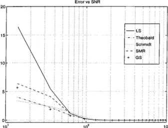
2.13 Estimation error versus SNR lor liea.st Squa.r(;s(LS), 'riuiobald,

Schmidt, Swaiiiy-Mehtci.-Rappoport(SMR) cuid Goldstein-Smitli(GS). 20

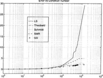
2.14 Estimation error versus kernel matrix condition number for Least Squares(LS), Theobald, Schmidt, Swamy-Melita-R.appoport(SMR.)

and Goldstein-Smith(GS)... 21

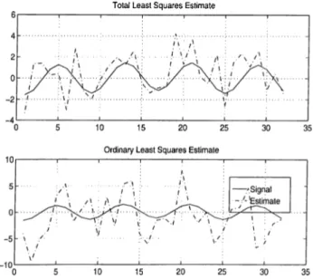
2.15 TLS and OLS %ctls = 31.2, %cols — 47.6 . 26

2.16 Effect of 6 on the R{A). 30

2.17 Application of Cadzow’s algorithm with SNR,=80dB and kernel of

low condition number, %error= 3 . 2 ... 31

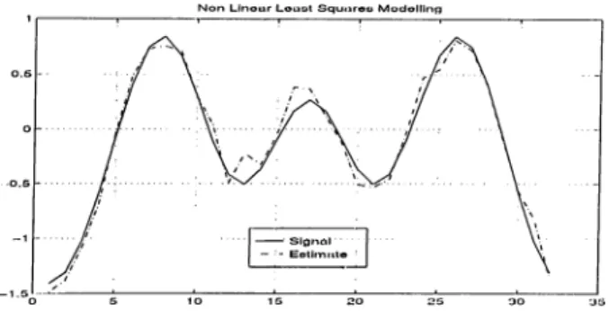
2.18 Non lineiu· least squares modeling algorithm with SNR,=28dB,

%error = 6 4 .2 ... 31

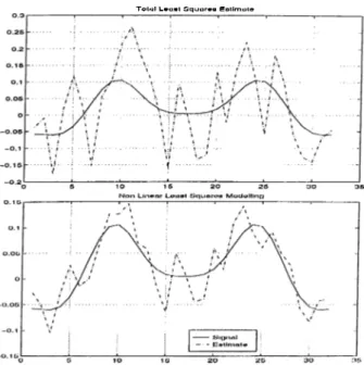
2.19 Comparing TLS and Nonlinecir Letist Squares Modeling, %error'i'LS —

71.5 and %erroi'cad = 24.1 32

3.1 Choice of Ridge Regression: increasing curve is tlie sample variance

of the fit error vector as a function of /i, horizontal line is a^. . . . 35

3.2 Error Dependent Ridge Regression(EDRR) with % error = 12.1

and Swamy-Mehta-Rappoport (SMR) with % error = 21.5 Esti­

3.3 Application of Gauss-Markov with recursive updates algorithni.

SNR=45dB and low kernel matrix condition number, %erroi — 2. . 41

3.4 Application of Gauss-Markov with recursive updates algorithm.

SNR=45dB and high kernel matrix condition number, %error= 8. 41

3..5 Fit Error and Magnitude of the estimate versus the number of

basis components... 47

3.6 Reconstructed estimate by using 10 components of the basis. . . . 47

3.7 WBR.R, FjDR.R, GM, SMR estimates, with %errorsi ('Wbrr ~

18.37, tEDRR — 15.23, eoM — 13.82, csmr = 24.54 ... 48

3.8 Estimation Error vs. SNR for the W BRR, EDRR, GM and SMR

estimates... 49

3.9 Estimiition Error vs. SNR for the W BRR and EDRR estimates. 49

3.10 Nonlinear Ridge Regression algorithm witli non linear minimiza­

tion technique. SNR=65dB, %error — 3 .1 1... 57

3.11 Nonlinecir Ridge Regression algorithm with non linear minimiza­

tion technique. SNR=46dB and k = 10'*, %error = 7.42 -57

3.12 NonlinecU' Ridge Regression algorithm with Gra.dient teclmique.

SNR=46dB, R - lOE %error = 3.24. 58

3.13 Maximum Likelihood-Bayesian approach, %error = 13.17... 59

3.14 Estimation error versus the bound vector norm... 59

LIST OF FIGURES X I V

.'{.15 Least Squares-Bayesian approach, %error = 12.75... 59

3.16 Nonlinear Least Squares Modeling, %error = 24.36... 60

3.17 Nonlinear Ridge Regression Modeling with non linear optimiza­

tion, %error = 16.7... 61

3.18 Nonlinear Ridge Regression Modeling with gradient descent mini­

mization, %error = 15.9... 61

3.19 Likelihood Bayesian approach, %error = 21.8. 61

3.20 Estimation Error versus SNR for the presented algorithms; (Jad-zow(Cad), Nonlinecir Ridge Regression(RR), Nonlinear Ridge R o gression with Gradient descent algorithrn(Grcidient), Bayesian-

Chapter 1

IN T R O D U C T IO N

The basic job of an experimenter is to descrilse what he or slie sees, try to explain what is observed and use this knowledge to helf) answer ([uestions encountered in the future. The explanation often takes the form of a irhysical model, which is a theoretical explanation of the physical phenomenon under study. Models make it possilrle to explore situations which in the actual system would bo; lia.xardous

or demanding. Aircra.ft and space vehicle simulators are well known exam]3les.

A model is usually expressed verbally first then formalized into one or more; equations giving rise to the mathematical model. A characteristic of science is its use of mathematical models to extract the essenticils from compliccited evidence and to qinmtify the implications.

An important reason behind modeling is to provide the required Framework for the estimation of the unknowns. Experience has shown that no measurement, liowever Ccirefully made, Ccin be completely free of errors. In science the word

Clmpter 1. INTRODUCTION

“error” does not carry the usual connotations of mistal<e. Error in a scientific measurement means the inevitable uncertainty that attends mecisurements. (Jn- certainty is not the ignorance of outcomes. As a matter of fact when a coin is tossed, we are certain that one of two outcomes will occur. What is not known is

heads or tails. Again, when a die is tossed, it is certain that 1, 2, 3, 4, 5 or 6 will

turn up. What is not known is which of these numbers. The future outcome of a. coin toss or a die toss is not only unknown l^ut also not knowable in advance. Thus uncertainty is the certainty that one of several outcomes will occur; but which specific outcome will prevail is unknown and unknowable.

A basic problem that arises in a broad class of scientific disciplines is to perform estimation of certain parameters from a model within uncertainties. In this thesis, we treat this problem when the model is a linear statistical one, which is described by:

A x = y , (1.1)

where x is the unknown vector, y is the measurement vector and A is the measui’ement kernel. As mentioned previously, there are no measuix'ments frex; of cM-ror, l,he obtained data presented in the vector y are considered to Ixi erroneous. An additive noise vector n is added to the observation to stress tliat fact. 'I’he uncertainty could come from the kernel matrix A , the entries of tins matrix are also subject to sampling errors, measurement errors, modeling errors and instrument errors. Again the matrix A could depend on an unknown real valued set of parameters 6 belonging to a set S. This is the case of array signal processing applications where $ refers to direction of arrivals of signals. Thus the problem we are dealing with is estimating an M dimensional vector x from an N dimensional

Chapter 1. INTRODUCTION

data vector y with:

y = A {6 )x n

(1.2)

In chapter 2, some of the commonly used approciches to tlie estinuition of the nnknowns in the presence of measurement uncertainties will be presented. In chapter 3, we will introduce the proposed approaches to the estimation problem. In order to compare the estimation performance of the old and new approaches, extensive simuhitions are provided throughout the thesis.

Chapter 2

Commonly Used Estimation

Approaches

2.1

Introduction

'riie commonly used approaches to estima.te the unknown parameters from a model under uncertainties are presented in this chapter. Over synthetically gen­ erated excunples, these approtiches are compared with each other in terms of their performances. In the Ibllowing, measurement relationship is modeled as:

y = A {9 )x + n , (2.1)

wliere y is the A-dirnensional vector of available measurement data., A is the measurement kernel or operator, x is the Tl^f-dirnensional unknown vector, n is the additive rnecisurement noise cind 6 is /^-dimensioned vector para.m(;t(u-ixing the uncertainty in the model.

We shall start by providing the approaches used for a fixed 6 , that is to solve the overdetermined set of equations:

CImpter 2. Commonly Used Esthmition Approaches 5

y = A X + n ■ (2.2)

W(' will investigate the Least Squares approach, then the ridge regression esti­ mate. For the model uncertainty ¡problem which is characterized by eqiuition 2.1, we will consider the Totcil Least Squares estimate and the nonlinear least squares modeling cilgorithm.

2.2

Known Measurement Kernel

2.2.1 Least Squares Fitting to the Measurements

The least squares method of estimation is extensively utilized in a wide variety of applications such as communications, control, signal processing and numerical analysis, since it requires no information on the statistics of the data, arid it is usually simple to implement. As we will see, it provides reasonably good estimates when the condition number of A is relatively small and the signal to noise ra.tio

of the mecisurements is high.

In the method of lecist squares, we want to find an estimat(.' x sucli tliat the norm of the fit error

e = y — A X (‘•^••1)

Chfipter 2. Commonly Used Estimation Approaches

lie least squares estimate satisfies the well known norrnaJ equations:

{ A ’^A) x ns = II (2.4)

n { A^ A ) is lull Tciiik then the least squares solution can be tbuncl as:

x l s = { A A ) '■A ’’ y (2.5)

When { A A ) is rank deficient, the least squares estimator is given by:

Xlss = A , (2.6)

where A 1’ is called the pseudo-inverse or the Moore Penrose generalized inverse ol A , which can be obtained from the singular value decomposition (SVD) of A .

When the measurement noise vector has independent identically (listril)uted normal entries, the least squares estimator cdso corresponds to the maximum like­ lihood estimator. The maximum likelihood theory is widely applied to a number of important applications in signal processing such as system identification, ar- ra.y sigiml processing and signal decomposition. It is also ap];)lied to find an estimate to uncertain model parameters. The principle of maximum likelihood is

illustrated by the following example [1].

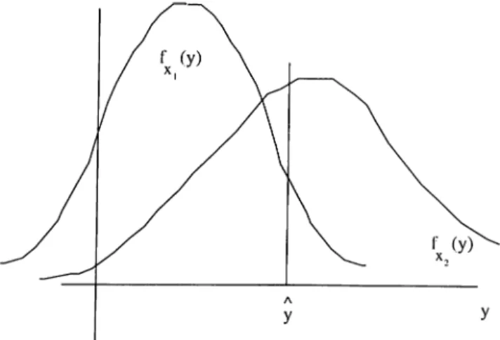
Let y be a random variable for which the probability density function /,■(;(/) is parameterized by an urdaiown parameter x. A typical density function is given

in figure 2.1. In this figure two densities are illustrated, one for parameter ;ri and

one for parameter X2- Suppose that the value y is observed. Based on the prior

model fx(ij) shown in 2.1 we can say that y is more probably observed when

X — x-2 than when x = .Ti. More generally there may l)e a unique value of ;r

Chiiptev 2. Commonly Used Estimation Approaches

Figure 2.1: Mcixiimmi Likelihood principle:Typical density functions.

X that makes y most probable, or most likely, the maximum likelihood estinmte

Xm l

-Xm l = argm ax./;.(?/) . (2.7)

We obtain the maximum likelihood estimate by evakuiting tlie conditional density ,/V|.Y(y/|-c) at the value of observation y and then searching for the value' of x that

maximizes f Y\x{ y\x) . The function /(.c,?/) = f Y\x{ y\x) is called the likelihood

lunction and its logarithm L(x, y) = In fy\a-iy\x) is called the log likelihood function.

In our problem we have N olrservations summarized in tlie vector y ol)tained l)y this relation:

y = A x + n , (2.8)

with n noriTicdly distributed having zero mean and covariance matrix R , the conditional probcvbility density function of y given x is:

Clmpter 2. Commonly Used Estimation Approaches

where \R | denotes the deterininant of R . The corresponding log-tikeliliood

fniiction is;

L ( x , y ) _{in fy\x (y\x)}

N i l

=

- Y l n 2 7 r - - l n \ R \ - - { y - A x f R - ' ( y - A x ) .

likelihood function with respect to x and setting it to 0, yielding:

XML = { A ^ R - ^ A ) - ^ A ’^^R-^y (2.10)

As pointed Ccirlier, the maximum likelihood estimator coincides with the least squares estimator when R = cr;^ J .

In tlie remaining of this sul^section we will investiga.te tlie mea.n and cova.ria.nce

of tire least squares and maximum likelihood estimators. Let 7Z(A ) be the

subspace spanned by the columns of A . ff we call y j the i)rojectiou of y onto

'R.{A) and y-2. the projection of y onto the orthogonal complement of 'R{A ),

then y j — A x belongs to 'TZ{A ) and is orthogonal to y 2· ilence we can write :

C =

||y

(

.

)

which attains its minimum when ||y 1 — A x\\^ is minimized with respect to x .

Since we Ccui alwciys find an x satisfying A x = y \ and it is unic|ue if and only if

mdl{A) = { x ; A x = 0} = 0 , (2.12) then, the least squares estinicite always exists, and it is unicpie if and only if A is full column raidv. The statistical behavior of cui estimator can be investigated l)y finding its mean and covariance. Assuming that the additive mea.surement

Cbcipter 2. Commonly Used Estimation Approaches

noise vector is zero mean, the expected value of the least squares estima.tor can Ije found cis:

E {x l s} = E { i A ^ ^ A ) - U ^ ^ y }

= E { i A ^ ^ A ) ~ ^ A ' U A x + n ) }

= (A " A ^^A )x + (A ^-^A ) - ' A }

= X ,

which implies that the least sqiuires estimator is unbiased. The covariance of the leiist squcires estimator is given by:

Cov{x l s} = E{(X LS - E{X Ls})(x LS - E{ x is}Y^} ■ (2.13) With the assumption that the noise vector n is normally distributed having zero

mean and covariance matrix R „„ = <7,^/ , the required computation can be

performed ecisily, yielding:

Cov{x l s} = crliA^^A) ' (2.14)

Mow much an estimator could deviate on the average from the actual parameters is given by the Mean Square Error (MSE) criterion. This is obtained by:

M S E {x l s) = trace(C't>u{«/^,s’ })

M ^

= cr„

i=l

(2.15)

where s/Xi is the singular value of A . Hence, if tlie matrix kernel has a. high

condition number then the MSE will be large.

Another criterion to quantily statistical performance of estimators, is com­ paring their error covariance matrix with the (Jramer-Ra.o lower bound, which

Chapter 2. Commonly Used Esthmition Appronches ₁₀

e.sta.blishes a lower IdouiicI on the covariance matrix for any estimator of a param­

eter. I he Gramer-K,ao theorem states that il y is an N -climensionaJ vector with

probability density function j y (y |a;) and the estimator x is an unbiased

estimator of x , then the error covariance matrix of x is bounded as ill.

C l{{x — x ) { x — x y ^ ] > J _(2.16)

where J is called the Fisher information matrix and it is given by:

= J^{[- ^^^Kfy\x{y\x)][- ^lnJy\x{y\x)f] . (2.17)

For the Least Squares estimator, the Fisher information matrix becomes:

J = — ^ . (2.18)

^ n

Thus, the covariance matrix of the least squares estimator given in equa­ tion 2.14 meets the Crarner-Rao lower bound. Hence, when the measurement noise is identically independently distributed normal, the least squares estimator is the best linear unbiased efficient (BLUE) estimator.

2.2.2

Ridge Regression

In 1970, Hoerl and Kemiard showed that based on the Mean Squarci Error crite­ rion, a biased estimation procedure could yield better parameter estimates of a.

linear model than the aricilogous estimates obtained via classical least sc|uares [2].

This procedure is introduced initially to avoid the ill effects of quasi-collineci.rity in ordinary least squares estimators. In order to avoid widely oscillating esti­ mate's of least squares, obtained in the case of measurement kerneds with a la.rge

Chapter 2. Commonly Used Estimation Approaches ₁₁

condition number, a penalty term on the weighted magnitude of the estimated variables is incorporated to the ridge regression cost function:

C = e e + X “ D XH , (2.19)

with e = y — A x and D — diag{ki),i = where the weights k-i > 0 are

known as the ridge regression constants. The Ridge Regression estimator, x nn, can be found as the uniciue minirnizer of the above cost function resulting in:

XRR - ( A^ ^ A + £ ) ) - ' A " y-1 A H. (2.20)

Similcu· estimator wiis obtained by Levenberg(1944) and Marquct.rdt(1963) in de­ veloping an algorithm lor nordinear least sciuares minimiza.tions [3]. In the pres­ ence of little or no prior information, the choice of the ridge regression constants becomes a difficult task. Therefore in many applications the weights a.re all cho­ sen to be the same, reducing the search spaee lor the right set of para.meters to oiKi. This case of unilbrm weighting is known as ordinary ridge regression arid its corresponding estimator is:

XORR = ( A " A + A: / ) - ' A " y

The expected value of the ridge regression estimator can be found as:

E {x r r} = E{{ A^^A + D ) - ^ A ‘^y}

=

(2.21)

which has a bias oh

E { x - X rr} = V diag(

k

Chapter 2. Comnionly Used Esthmition Approaches 12

where V is the right singulcir matrix ¿uicl v/Ai’s ¿u-e the singular values oF the A matrix. Likewise, the covariance of the Ridge R.egression estimator ca.n be found as:

XI

c o v { x m } = diag( )V " ,

(A^ + kiy^ (2.23)

where (jj; is the noise veu-iance.

Since the Generalized Ridge Regression is a biased estimator, we use the Cramer Rao lower bound for biased estimators :

0

Cov{xjir} > [ - ^ E { x J Rji}]

where J is the Fisher information matrix for x . since

A'^ Cov{x r r} = a^V die

(Aj· + ki)

H

l E i x n . ) = V d l a g ( ^ ) V " .

it can be shown that:

J =

d

- Y ^ E {

8

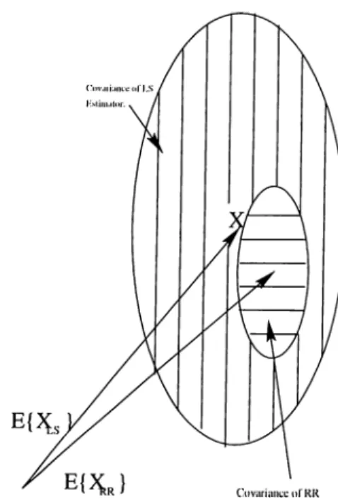
The main task in Ridge Regression estimators is how to choose the Ridge Regression constants. The criterion that we are using to judge estimators is the Mean S([uare Error criterion, so the Ridge Regression estimator would outperform the Least Squares estimator if :

Clmpter 2. Commonly Used Estimcition Approaches ₁₃

Figure 2.2: Least; Squares and Ridge Regression Estimators: Bias and Covaruuice.

In other words we would like to get the situation illustrated l>y figure 2.2. 'riie

corixisponding Mean Square Plrror of the Ridge Regression (Estimator is:

\1I I

MSE(x r h) = E { { x , m - x Y \ x , m - x ) }

(2.30)

fet i^г + k Y iXi. + k y ·

Theobald proved that to provide the condition in e(|uation 2.29 we should liave :

V ‘' x ^ ^ x V , /2 1

— 3 — « ‘ '' “ « h + x ' ’ (2.31)

which is satis.iiecl tor ki > 0 or ki < —2\i for i — When tlie are

fixed, the domain of parameters where the genei’cilized ridge regression estimator is better than the least squares one ¿ire given

* " V d i a g ( - ^ ) V " a ! <

k \

2X + k'

which is an ellipsoid. Several suggestions were proposed Idr the choice of tlie ridge regression constant: Goldstein and Smith (1974) proposed to take ki =

Chapter 2. Commonly Used Esthmition Approciches 14

~ ^ where 7 = [4]. Schmidt (1976) suggested tha.t k could

2

1)0 taken as k = ■ Swamy, Mehta cuid Rappoport (1978) sliowed tlurt if a.

priori information about the norm of the pcirameter vector x is provided then we can get better estimates. For instance, if we suppose tlial. x lies in a hyper-spa.ce of radius r, that is

X ^^x < < 00 , (2.33)

the value of x thcit minimizes subject to equation 2.33 is:

xsMRik) = (A " A + a l k I ) - ^ A ‘' y , (2.34)

where :

a.nd

k = c\j.

y^^ Qy (2.35)

Q =

“ + { N - M)-^A

” A

“

with c a. positive constant and the noise variance.

(2.36)

2.2.3

Simulation Results

In the simulations we generate randomly a iricitrix A , a. vector x and a Caussian i-a.ndom vector n then we find the ol^servation vector y liy

y = A X + n (2.37)

Then, based on A cUid y we apply the algorithms desci'ibed in this chapter to find an estimate for x . All through the simulations we will give the (istimation error values for an estimate x of x by error percenta.ge: %error =

Clmpter 2. Commonly Used Esthmition Approaches ₁₅

In iigures 2.3- 2.7, the estimated and actiuil x obtained using the method of Ix;ast Squcires and also methods proposed by Theobald’s, Schmidt’s, Swamy- Mehta & Rappoport ¿uid Goldstein are shown. In this simulation the kernel

matrix hcis a condition number k < 10 and the signal to noise ratio, SNR =

—2 0 1 o g (^ ), is 80dB. As expected lor such a Ccise the least squaix^s estimator is performing well, the estimate is very close to the true unknown Vcirialiles. The estimates obtained via the proposed ridge regression procedures provide very close results to the theoretical values. In such cases, one would prefer to use the Least Squares estimator since it does not need any prior knowledge on the noise or data statistics, and the inversion ol the system matrix AA^'^ can be performed without any trouble.

However, as shown in iigures 2.8- 2.12. when the signal to noise ratio de­ creases below 40dB a Ridge Regression estimators provide far more accura.te results. This is beccuise of the fact that the least squai'e estimator is more sen­ sitive to the measurement noise. The lecist squares estimate is more noisy along the right singular vectors corresponding to the smaller singular values. Since,

t3q:)ically sniidler singuhu· viilues are associcited witli oscillatory singular vectoi's,

the estimates obtained at low SNR Imve widely oscillatory behavior as shown in

figure 2.8.

In order to obtain stcitisticcilly more significant comparison results, we re- l)cated the above comparisons for various realizations of y at different SNR val­ ues, and plotted the average errors in the obtained estimates in figure 2.13. At each SNR. value 25 different realizations have been used. As it can l)e seen, performance of the least squares estimator degrades badly at low SNR values

Chcipter 2. Commonly Used Estimation Approaches 16

compared with the results obtained by the ridge regression family of estimators.

In order to test the performance of these estimators in tlie case of measure­ ment kernels with high condition numlser, we compared the pertbrmances of the estimators of Vcirious condition numbers. In figure 2.14, for each estimator, we |)lotted the avei’cige error norm as a function of the kernel condition number. As seen from this figure, the performance of the least squares estimator degrades drastically as the condition number gets large.

The superiority of the ridge regression estimators over least squares is due to the utilization ol aviiilable prior information. The methods presented by Theobald, Schmidt, Swamy Mehta, cind Rappoport, a.nd Goldstein outperform least squares when the noise sta.ndard deviation and the magnitude of the un­ known vector cire available. Unless a priori knowledge about tlie signal and the noise statistics are provided, the performance of the suggested ridge regression estimators deteriorates. From the performance of the Ridge Regression estima­ tors we can also conclude that Swamy, Mehta, and Rappoport’s give Iretter results than the other estimators.

Chapter 2. Commonly Used Estimation Approaches 17

T h o O L S E s tim a t o

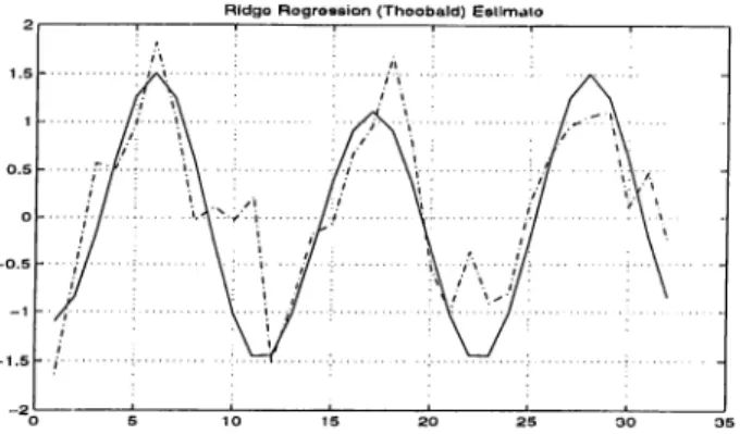
R id g o R o g r o s s io n ( T h e o b a ld ) E s tim a to

Chapter 2. Commonly Used Estimation Approaches ₁₈

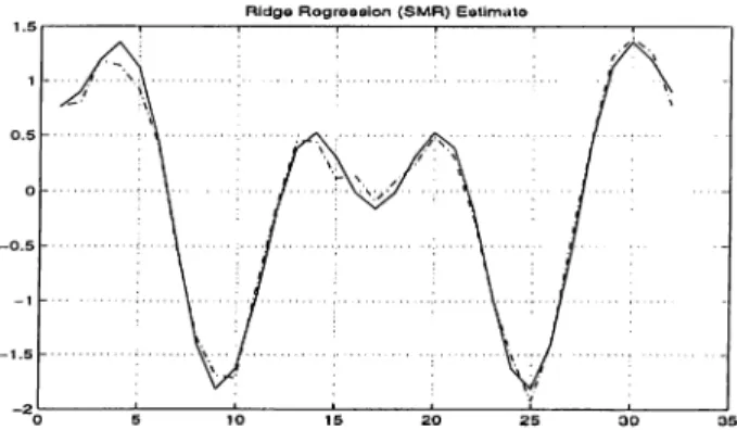
R Id g o R o g r o s s io n ( S M R ) E s tim a t o

Figure 2.6: Swaray Mehta and Rappoport Estimator, % error= 4.45. R id g o R o g ro B s lo n ( Q o ld s t e i n ) E s tim a t o

Figure 2.7: Goldstein Estimator, % error= 11.46. T h o O L S E s ti m a t o

Chapter 2. Commonly Used Estimation Approaches ₁₉

R Id g o R o g r o s s io n ( T h e o b a ld ) E s llm a t o

R id g o R o g r o s s io n ( S c h m i d t) E s tim a t e

R id g o R e g r e s s io n ( S M R ) E s ti m a t e

Chapter 2. Commonly Used Estimation Approaches 20

R id g o R o g r o s s io n (G o ld a t o in ) E s ti m a l o

Figure 2.12: Goldstein Estimator, % error= 26.8.

Error vs SNR T~r~l---;— LS i :--- Theobald; Schmidt : i - - SMR ; : + GS;

Figure 2.13: Estimation error versus SNR for Least Squares(LS), Theobald, Schmidt, Swamy-Mehta-Rappoport(SMR) and Goldstein-Smith(GS).

Chapter 2. Commonly Used Estimation Approaches 21

Error vs Condition number

Figure 2.14: Estimation error versus kernel matrix condition number for

Least Squares(LS), Theobald, Schmidt, Swamy-Mehta-Rappoport(SMR) and GoIdstein-Smith(GS).

2.3

Uncertain Model

In the pi'evious section, the measurement matrix entries are assumed to be known exactly, hence, the only source of uncertainty in the observcition vector y is the additive noise vector n . However this assumption is often unrealistic. In prac­ tice, we seldom face an exactly known measurement kernel. Errors that do take place during modeling cuid sampling may imply iiiciccuracies on the measurement matrix A ¿is well. The inaccuracies in A can be due to uncertainties in a few pcirameters which define A , or to the uncertainties in each individual entry in

A which do not fit to a low order parametric description. In the latter case the

Totcil Least Squares (TLS) is one of the commonly used methods of obtaining estimates when there are errors in both the observation vector y and the data matrix A . Although computationally more intensive and limited in terms ol its cipplication areas, nonlinear least squares modeling is the method ol choice il there is a parametric description of the measurement matrix.

Chapter 2. Commonly Used Estimation Approaches 22

2.3.1

Total Least Squares

The I ’otal Least Squares approach has been introduced in recent years in the nuniericcil analysis literature as an alternative for the least squares in the case that l)oth A and y are affected by errors. A good way to introduce the 'Total Least Squares method is to recast the Ordinary Least Squares problem.

In the Least Squares estinicition, the unknown x is obtained as the rninimizer of the following optimization problem:

mm

y'çRM \y - y

II

Subject to y ' ^ TZ(A ) .

Once y is found, the minimum norm x satisfying A x = y ' Is called the Least S(|uares solution, 'riie underlying assumption here is that errors only occur in the vector y and that the matrix A is exactly known, which is often far from reality. 'The least squares estimator is obtained by solving the smallest perturbation on the measurements so that the perturbed measurement will lie in the range space of A . When there cvre errors in both A and y , the same idea of perturbation can be applied to both A and y such that the perturbed measurements will lie in the range space of the perturbed A rmitrix. Again we want to find the minimal perturbafion on both A and y . In the TLS, this is achieved by finding the solution to the following optimization problem:

, min \\[A, y]-[A, y]\\i. ·

[A

Subject to y E TZiA) ,

where ||.||f denotes the frobenius norm. Once a. minimizing [ A , y ] is found, x

Chcipter 2. Commonly Used Esthmition Approaches 23

To solve this problem, we bring A x ^ y into the following foran

[ A, y ]

X

- 1

0 . (2.38)

Let [A , y ] = U S V he the singulcir value decomposition of [A ,?/], with

U = «M + l] ,

S = diag((Ti,...,(rM+i) ,

If ctm+1 7^ 0 then [A ,y ] is of raidi M + 1 cuid the subspace S generated by

the rows of [yt ,y ] coincides with and there is no nonzero vector in the

orthogonal complement of <?, hence equation 2.38 is incompatible. 3b obtain a solution the rank of [A , y ] must be reduced to Ad.

value

r r= rariKk{C ). if k < r and C k = ^¿=1 ¡v j then

and

mm

rank(D ) = k

min ||C — D ||;r

ratik{D ) = k \C - C =

says: Let the singulcU’

= E;'l=\0-iUivl with

(^k+i (2.39)

P

E

1

with p = min{M, N). Using this theorem, the best rank Ad 'Ibtal Least Squares approxinicition [ A , y ] of [A , y ] which minimizes the deviation in variance is given by:

jter 2. Commonly Used Estimation Approcichef.is 24

where S — cl i ag( ( Ti , <j m, 0). It is clecir that the approximate set

[ A , y ]

X

-1

0 (2.42)

is compatible cincl its solution is given by the vector v the last column of V .

'I'lius the total least sc^uares solution is : - 1 X TLS = II A _2 = ( A ‘‘ A [ y 1,M+1,· · · ,^ M,M + i ,2 M+l \T _(2.43) (2.44)

(xxists and is uniciue solution to

A x = y (2.45)

Whenever V m+i,m+i 0, the Total Least Squares solution is solvable and

is therefore called generic. Problems may occur if <jp > (jp+i = ... = (Tm+i for

p < M and if all V M+i,i = 0 for i = p + 1,..., M + 1 these prolrlems are called non generic .

libr the generic case when ap > cr,;+i = ... = o'm+i lor p < 7V/, if not all

Y = 0 for i = p + 1,..., 714 + 1 then the minimum norm Total Least Squares

solution is given by:

- 1 M+i

X I LS Y^A/+1 TT 2 T (2.46)

M+Ia i=p+i

For the non generic Ccise when V M+i,j — 0 foi' j — P + 1, ···, At + I · H > <y,>

and y M+x,p 7^ 0 Total Least Squares Solution is given by:

- 1

xtls =

M+l,p- [ y 1,;;, ■··, y M,p] ‘

Chapter 2. Commonly Used Estimation Approaches 25

2.3.2

Simulation Results

'lb test the performance of the Total Least Squares Estima.tor, we generated matrix A „ of independent identically distributed ra.ndom variables, with zero mean, 'riiis matrix is added to the kernel matrix A , then we generate the data vector y in the same way we did for testing Ridge Regression and Least S(|iuires estimators.

Figure 2.15 shows the Total Least Squares (TLS) and the Ordinary Least Squares (OLS) estimiites when applied to a case where the Total Least Squares solution is generic. The Total Least Squares outperforms the Least Squares for several reasons. Ordinary Least Squares takes into account only errors in the ol:)served data y . However, Total Least Squares considers that Irotli the data, vector y and the kernel matrix A cire erroneous, and it searches for the smallest jrerturbation on both A cind y to reach a compatil)le set of equations.

'I'he main problem in using the TLS approach is how to determine the rank of the augmented matrix [A , y ] and how to choose p for which cr,, ^ 0. 'The perlbrmance of the TLS estimator deteriorates drastically when the rank is chosen inaccurately.

Despite this drawbcick, the 'Lotal Least Squares estimate remains the ordy wa.y to solve the problem of linear parameter estimation under model uncertainties that are treated as independently distributed random variables.

Chapter 2. Commonly Used Estimation Approaches 26

Total Least Squares Estimate

Figure 2.15: TLS and OLS Voctls = 31.2, %eo^,s = 47.6

2.3.3

Nonlinear Least Squares Modeling

In niariy applications of interest the phenomenon under investigation can be rep­ resented by a system of linear equations in which the elements of the system matrix are known functions of a. set of parameters. For instance, in array sig­ nal processing the parameters correspond to direction of arrivals of the received signals, or in inverse prol:)lems, the parameters correspond to the measurement device geometry. For these cases measurements relation is modeled as:

y = A (6 )x + n , (2.48)

where 6 € 7^^ is a vector containing P parameters characterizing the uncert in the model. To solve this problem the Nordinear Lecist Squares Modeling tech­ nique has been applied [5]. In this approach, which was presented by (Jadzow, a selection of the parameter vector 0 and the unobserved vector x are tried to be found so that A { 0 ) x best approximates y in the Euclidean norm sense.

Chapter 2. Commonly Used Estiimition Approaches 27

More precisely, 0 and x are found by solving the ibllowing squared /2 norm

optimization problem:

min min 11« — A i d )x\U (2.49)

Due to the nonlinear fashion in which x and 6 appear, generally there is no closed form expression for the solution to this optimization problem. So it is necessary to apply nonlinear optimiziition techniques to search fbr a solution. The secU'ch space dimension can be reduced to the dimension of 6 by observing that the optimal value of x given 6 is:

X IS = A \ e ) y (2.50)

Hence, the overall optimization can be recast in terms of 6 alone as:

min ||[J - P { 0 ) ] y f

0€R^

( 2 M

where P ( d ) = A ( 9 ) A H 0 ) is the projection operator onto the range of A (9 ).

Since I — P (9) IS the projection operator onto the perpendicular space ol range

A ( 9 ), optimal value of 9 Ccui be found as the niciximizer ol

y ( 9 ) = I I P ( 9 ) y (2.52)

Thus we would chose 9 so that the projection of y onto the subspa.ce spanned by the columns of A (9 ) has the maximum squared norm.

The maximization of g { 9 ) necessitates a nonlinear programming algorithm to approximate an optimal solution. Cadzow suggested the method ol descent in which the present estimator 9 is cidditively perturbed to 9 + 5 , where 6 is relerred to as perturbation vector. The basic task becomes to selec t the peitui l)ation

Chapter 2. Coiinnoiily Used Estimation Approaches 2 8

vector so that the improving condition

g{d + 6 ) > (j{e ) (2.53)

is satisfied. For a sufTiciently small, in size, perturbation vector, a. d'aylor series expansion, of the perturbed criterion can be made, in which only the first two terms are retciined:

g{e-^6) = \ \ p { e + 6 ) y f

,

a,nd 6.j or Oj are the entry of 6 or 6 , respectively. A logical choice of the

perturbation vector would he one that niciximizes the Euclidean norm criterion given by equation 2.54.

< / ( « + « ) = .,(«) + i " i ( « ) ' ' p ( # ) a

+ a " P ( Û )L ( 6 ) 6 + 6 "l (6 ) " £ (6 ) 6 .

By setting the gradient of this expression, with respect to 6 , to the zero vector the optimal selection can be found as :

« · = - [ » { £ ( « ) " £ ( # ) ) ) » « { £ ( « ) " P ( « ) a ) . (2.56)

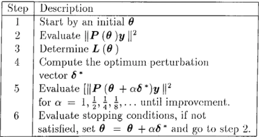
To ensure a sufficiently snicill perturbation, a scaled perturl)ation vector a6* is instead used. The nonlinear programming algorithm is given in table 2.1. The stopping condition to be evakuited is the fit error norm.

Chcipter 2. Commonly Used Estimation Approaches 29 Description

2

Compute the optimum perturbation vector 6 *

Evaluate [||jP (Û + *)y |P

for o; — 1, . until improvement.

Evaluate stopping conditions, if not

satisfied, set 9 = 9 -\- ct9* and go to step 2.

Table 2.1: Nonlinear Programming Algorithm.

2.3.4

Simulation Results

Consider the Ibllowing matrix:

1 0

AiO) = 0 cos(d) . (2.57)

0 sin(t^)

The rcuige of this matrix is a plane in the three dimensional space. The parameter

9 determines the slant angle of the plane as shown in figure 2.16. Based on

the above pariimetric representation we investigate the the performance of the

nonlinear least sciuares modeling estimator. So, we choose a random 9 then

generate x and n in the previously described fashion, and we obtain y by

A (9^)x + n . Then, based on y and the known parametric description of A , we estimate x . Eigure 2.17 shows the result obtained in the case when the system is nearly noise free SNR = 80dB. The nonlinear least squares modeling algorithm converges in few steps to the optimal vector of unknowns 9 and tlu? (;stima.te x is very close to the true unknown vector.

Cluipter 2. Commonly Used Estimation Approaches ₃₀

However in the case when we increase the signal to noise ratio the quality of the estimates deteriorates and the estimated parcimeters deviate significantly from the true values. This is because in the search for optimal d that results in the largest projection o i y onto the subspace spanned by A( 0 ), the additive noise

vector is also projected. Hence, if the condition number of ) is large, the noise

component of the projection may result in significant estimation errors along the singular vectors corresponding to the smaller singular values, as illustrated by figure 2.18, where the SNR = 28dB. This is due to the fact that this algorithm is lra.sed on the least square estimator, and whatever the least squares sulfer from will be inherited in this procedure.

Chapter 2. Commonly Used Estimation Approaches ₃₁

Figure 2.17; Application of Ccidzow’s algorithm with SNR=80clB and kernel of low condition number, %error= 3.2

A comiDarison between the performance of Total Lecist Square,s and Nonlinear Leaat Squares algorithms is held in figure 2.19, both estimates were applied for the ca.se of an SNR 47dB, the results show the superiority of tlie Nonlinear Least Squares Modeling. I'hus modeling the uncertaintj^ of the kernel matrix as a function of nuisance parameters will improve the quality of the estimate.

N o n L In o a r L o a o t S q u i i t e o M o d e l lin g

Figure 2.18; Non linear least squares modeling algorithm with SNR=28dB, %error = 64.2 .

Chapter 2. Commonly Used Estimation Approaches ₃₂

T o t a l L e a n t S q u a r e s E a tim u te

Figure 2.19: Comparing TLS and Nonlinecir Least Squares Modeling,

Chapter 3

Proposed Estimation Methods

3.1

Introduction

In the i^revious chcipter we presented the coniinonly used estimation a.|)|)roa.ches in the presence ol’ rnecisurernent uncertciinty. We investigcited tlie Least .Scpiares and Ridge Regression estimators for the fixed kernel case. The drawl)acl'Cs of these approaches were observed in the simuhitions, due to noise standard devi- a.tion and the structure of the data matrix for the fonrier; and to the necessity of irrior information for the choice of the ridge regression constant for tlie latter. For the uncertain kernel case we examined the Total Lc!ast Sciuai es a.nd tlie Non­ linear Lecrst Squares Modeling approciches. In this chapter, wc will present new approaches to provide more reliable estimates of the unknowns.

Following the scune plan as the previous chapter, we start by |)roposing the methods that we can apply when we fix the parameter 6 and wo assume that

Clmpter 3. Proposed Esthmüion Methods 34

it is known. Then we present cilgorithms when this paraineter is unknown and need to l^e estimated as well.

3.2

Known Measurement Kernel

In this section, we will present a way to choose the Ridge Regression constant l:)y constraining the estimate to lead to ci fit error helving the same statistics cis that of the cidditive noise. Then, we introduce a method that alleviates the necessity of a. priori information by iteratively estimating the noise and the signal variance. 'Idien, we propose an algorithm to solve large linear system of equations, the aigorithm recursively updates the solution in an increasingly larger dimensional subspace whose basis vectors are a subset of a complete wavelet basis.

3.2.1

Error Dependent Ridge Regression Constant

As presented in the previous chapter. Ridge Regression methods provide a. fam­ ily of solutions depending on the regression parcimeter. Some of the commonly used ways of choosing the ridge regression parameter have been presented in the previous chapter. However no firm recornmendcition for optimal Ridge Regres­ sion parameter seems to emerge. The simplest single parameter family of ridge regression estimates are in the following form:

Chciptei· 3. Proposed Estimation Methods 35

where p is the regression parcimeter.

Different methods of choosing p will lead to different fit error vectors

6 imip) = y — A X rr(p). If there is prior information on the statistics of

the random noise vector, one can try to choose p such that e rr{p) will look like

a realization of the random noise vector. The similarity can be measured based

on the devicition of sample moments of e rr(p) from the known moments of the

noise vector. In practice, only the first few moments can l)e used for tins purpose.

Here we suggest to choose p such that the sample variance of e rr(p) is the same

cis the noise vciricince.

3.2.2

Simulation Results

Over a synthetically generated example, this practical approach is compared with the Swamy-Mehta and Rappoport approach, and the obtained results are shown in figure 3.2. As seen from this figure, the perlbrniauce of the proposed ap­ proach is l)etter. This is a typical case over moderate sized problems. When the dimension of y gets larger, the performance difference gets smaller.

J MIcdio Houin

Figure 3.1: Choice of Ridge Regression: increasing curve is the sample variance of the fit error vector ¿is a function of p, horizontcd line is cr^.

Chcipter 3. Proposed Estimation Methods ₃₆

Figure 3.2: Error Dependent Ridge Regression(EDRR) with % error = 12.4 and SwaiTiy-Mehta-Rappoport (SMR) with % error = 21.-5 E.stirnate.s .

3.2.3 Gauss-Markov Estimate with recursive updates

There cire two fundainentally different way.? of .solving statistical problems: The classical and the Bcxyesian approaches. In the classical approach, a. set of data generated in ¿iccordance with some unknown probability law will be used without making any assumption about the urdinown law. In the Bayesian a|>|)roa.ch, the use of any reasonable prior knowledge about the unknown is recommended.

In deriving the maximum likelihood estimator we have iiderred the valiui of the unknown parameter x l:)y chasing x to be the parameter that maximizes the likelihood of the observed data y , this is a classical view of the problem. In the Ibllowing we will treat the unknown parameter x as a realization of a random experiment irom which the unknowns are endowed with prior distribution. This is the Bcxyesian approach where the information available prior to and carried by the measurements are optimally combined to obtain an estimate lor x .

If we define P{x \y) to be the conditional probability that x is true given y , tlien Bayes theorem gives the desired P{x \y) from the computal)le probcxbility

Chapter 3. Proposed Estimation Methods 37

probability because it is known in advance, somehow, to obtain y , and P{x \y) is called the a posteriori probability because it is what we aim to obtain after considering the above facts.

P{ y \x)P{x) P{ x \y)

P( y )

(3.2)

Let X B he the Bayes estimator. The quality of the estimator « b is measured by a real-valued function with some specific properties, known as the loss function, demoted by L[x , ®s ] . A typical loss function would be the quadratic one:

L[x ,x b] == [x - x b^^Ix ~ x b] , (3.3)

which assigns a loss equal to the Euclidean distance between the aetual value

of X and the estimated value x b- The Bayes estimator under (luadratic loss is

given by:

x b = arg min / L[x , x B].f{x\y)dx , (3.4)

X J

which is the conditional mean of x given y , that is

X b = P{x\y}

·

(‘hh)

Our problem is to estimate x Iroiri the overdetermined set of equations:

y = A X p n . (3.6)

Assuming that x and n are independent, zero-mean Gaussian random vectors, with autocorrelation matrices R xx and f 2 „ „ , respectively, we get the lollowing jointly Gaussian density for x cuid y :

X - N 0; . y . R XX Rx x A A R XX A R XX A P R n H (3.7)

(Jhciptcr 3. Proposed Estima.tion Methods 38

I b find the Bayesian estimator x b that minimizes the mean squared error, we

have to find the expectation of the random vciriable z — x \ y . Causs-Markov theorem states that if x cind y are random vectors that are distributed according to the multivcU’iable distribution

m. (3.8) X - N r r i x 1 R X X JFi, j.y . y . _ m . y _ R y x R yy (3.9) 'rhen the conditional distribution of x given y is multivariate normal:

P{x \y) ~ N { x , P ) ,

where the mean x and the covariance P cire given by:

X = m :, + i i xyR yyiy - r n y)

P = - R^y Ry y Ry : , .

I ’hus the Bayesian estimator for x is given by:

XB = ( A “R - ‘A + R - p - ‘A"R7.iy

In the case of x and n are composed of independent identically distributed

random variables, i.e., and = <T;|/,weget

(3.10) ‘Z XB = ( A " A + ^ / ) - U ' ^ y , P = < T ^ ( A " A + ) a2 n r \ — I (.1.11) (3.12)

Note that x b is ridge regression estimator with ridge regression constant p —

and the corresponding mean square error is:

_ 2 H M S E ix b) = trace(,r2 V aiag( - ) V “ ) = E M .1 ^ n ^ \i(xl + (3.13)

Chapter 3. Proposed Estimation Methods 39

which is smaller than the MSE of the maximum likelihood estimator due to the timal use of the prior information on x .

In the case of urd-cnown erf, and erf, we can first obtain thedr maximum likeli­ hood estimates and then we use them in the Bayesian estimator, d'he approach in developing the Bayesian estimator was to find ;

Xb = nvax F{ x\y) . (3.14)

I'he maximum likelihood estimator for z = can be obtained as:

z = arg max P y { Y = y ) (3.15)

If U is the left singular matrix of A , then ?/,„ = U^^y luis a normal distribution with zero mean and diagonal covariance matrix erf A-bcrf / where A is the dicvgonal matrix with entries which are the square of the singular values of A . Hence, the probability density function of y rn 1*^·

Jyini^rn) —

n

« e x p ( l g f e )

.=1 y'ijrCA.crJ + a'‘ )

Maximizing fy,n (Y m) with respect to z is equivalent to maximizing

N ,

_ ____ynil

L ·

(3.16)

(3.17)

'taking partied derivatives with respect to erf and erf we olrtnin:

dJ dal dJ dal ~ L · ^ y'ii ^i^'x -(3.18) (3.19)

Chciptei' 3. Proposed Estiimitioii Methods 40

To find the solutions tlicit annihilate these quantities we may use the successive substitution method, to get:

Er=

Where erf. _‘^'(A:) ¿md erf _'(A:) stand for the values of erf and erf at step k of the iterations.

VVe could also use a gradient descent method to successively converge to the solutions for af and erf.

3.2.4

Simulation Results

'I'o test the performance of the above proposed algorithm we make use of tlie same synthetic e.xample used in the previous sections. The results are shown in Figure 3.3 and 3.4. As seen from these figures, the estimator we suggested do not suffer from the multi-collinearity ¡problem in the kernel matri.x A because it belongs to the class of ridge regression estimators. The signal and noise variance estimation process in the Gauss-Markov with recursive updates algorithm ends up by converging to values tha.t cire within 10% ol the actual values ( af = 1 and erf = 0.92, af = 0.02 and df = 0.018 ). These results are plugged into eipiation 3.11 and the estimate that we obtain shows good perlormance which is robust to the noise standard deviation or kernel nicitri.x condition numlrer.

Chapter 3. Proposed Estimation Methods 4 1

Figure 3.3: Application of Gauss-Markov with recursive updates algorithm. SNR=4.5dB and low kernel matrix condition number, %error= 2.

Onuaa Markov wllli I'louuriilvu upciatou

Figure 3.4: Application of Gauss-Markov with recursive updates algorithm. SNR=45dB and high kernel matrix condition number, %erroi— 8.

3.2.5

A Wavelet Based Recursive Reconstruction Algo­

rithm

Reconstruction of the unknowns from the data has been tlie subject matter ol many inverse problems arising in a vast class of applications as geopliysical sig­ nal processing cind speech processing. A very important first step of the inverse problems is the parameterization of the unknowns. In many applications, where the sensitivity of the measurements varies across the space of the uidviiowns, the spa.ce of the unknowns is partitioned into cells of non-uniform sizes. 'I'he dimen­ sions of cells becomes larger when the sensitivity ol the measureriKnits to those