FEATURE POINT CLASSIFICATION AND
MATCHING
a thesis
submitted to the department of electrical and
electronics engineering
and the institute of engineering and sciences
of bilkent university
in partial fulfillment of the requirements
for the degree of
master of science
By
Av¸sar Polat Ay
August 2007
I certify that I have read this thesis and that in my opinion it is fully adequate, in scope and in quality, as a thesis for the degree of Master of Science.
Prof. Dr. Levent Onural(Supervisor)
I certify that I have read this thesis and that in my opinion it is fully adequate, in scope and in quality, as a thesis for the degree of Master of Science.
Assoc. Prof. Dr. A. Aydın Alatan
I certify that I have read this thesis and that in my opinion it is fully adequate, in scope and in quality, as a thesis for the degree of Master of Science.
Assist. Prof. Dr. Pınar Duygulu S¸ahin
Approved for the Institute of Engineering and Sciences:
Prof. Dr. Mehmet Baray
ABSTRACT
FEATURE POINT CLASSIFICATION AND
MATCHING
Av¸sar Polat Ay
M.S. in Electrical and Electronics Engineering
Supervisor: Prof. Dr. Levent Onural
August 2007
A feature point is a salient point which can be separated from its neighborhood. Widely used definitions assume that feature points are corners. However, some non-feature points also satisfy this assumption. Hence, non-feature points, which are highly undesired, are usually detected as feature points. Texture properties around detected points can be used to eliminate non-feature points by determining the distinctiveness of the detected points within their neigh-borhoods. There are many texture description methods, such as autoregressive models, Gibbs/Markov random field models, time-frequency transforms, etc. To increase the performance of feature point related applications, two new fea-ture point descriptors are proposed, and used in non-feafea-ture point elimination and feature point sorting-matching. To have a computationally feasible de-scriptor algorithm, a single image resolution scale is selected for analyzing the texture properties around the detected points. To create a scale-space, wavelet decomposition is applied to the given images and neighborhood scale-spaces are formed for every detected point. The analysis scale of a point is selected according to the changes in the kurtosis values of histograms which are
ex-non-feature points are eliminated, feature points are sorted and with inclu-sion of conventional descriptors feature points are matched. According to the scores obtained in the experiments, the proposed detection-matching scheme performs more reliable than the Harris detector gray-level patch matching scheme. However, SIFT detection-matching scheme performs better than the proposed scheme.
Keywords: Feature Point Elimination, Feature Point Matching, Digital Video
¨
OZET
¨
OZN˙ITEL˙IKL˙I NOKTA SINIFLANDIRMASI VE ES¸LEMES˙I
Av¸sar Polat Ay
Elektrik ve Elektronik M¨uhendisli˘gi B¨ol¨um¨u Y¨uksek Lisans
Tez Y¨oneticisi: Prof. Dr. Levent Onural
August 2007
Bir ¨oznitelikli nokta belirgin bir noktadır; etrafındaki di˘ger noktalardan ayrılabilir. Sık¸ca kullanılan tanımlarda ¨oznitelikli noktaların k¨o¸seler oldu˘gunu varsayılır. Ne yazık ki bazı ¨oznitelikli olmayan noktalar da bu varsayıma uyar. Dolayısıyla, istenmeyen ¨oznitelikli olmayan noktalar da ¨oznitelikli noktalar gibi algılanabilir. Algılanan noktaların etrafındaki doku nitelikleri ¨oznitelikli olmayan noktaların ayıklamasında kullanılabilir. Bunun i¸cin nok-taların etrafındaki doku ¨ozellikleri kullanılarak kom¸sularından ayrılabilirlikleri bulunur. C¸ ok sayıda doku betimleme y¨ontemi vardır, ¨orne˘gin, ¨ozba˘glanım modelleri, Gibbs/Markov rastgele alan modelleri, zaman-sıklık d¨on¨u¸s¨umleri, vs. ¨Oznitelikli noktalarla ili¸skili uygulamaların ba¸sarımlarını arttırmak i¸cin iki yeni nokta betimleyici ¨onerilmektedir. Bu betimleyiciler ¨oznitelikli olmayan noktaların ayıklanmasında ve ¨oznitelikli nokta sıralanması ile e¸slenmesinde kullanılır. Betimleyici algoritmasının bilgii¸slem y¨uk¨un¨u katlanılabilir bir seviyede tutmak i¸cin algılanan noktaların etrafındaki doku ¨ozelliklerinin ¸c¨oz¨umlemesinde tek bir resim ¸c¨oz¨un¨url¨u˘g¨u se¸cilmi¸stir. C¸ ¨oz¨un¨url¨uk-uzayı yaratmak i¸cin verilen resimlere dalgacık ayrı¸sımı uygulanmı¸stır ve her
¸c¨oz¨umleme ¸c¨oz¨un¨url¨u˘g¨u kom¸suluk ¸c¨oz¨un¨url¨uk-uzayından ¸cıkartılan histogram-ların kurtosis de˘gerlerindeki de˘gi¸simlere g¨ore se¸cilmektedir. Betimleyici kullanılarak algılanan ¨oznitelikli olmayan noktalar ayıklanmakta, ¨oznitelikli noktalar sıralanmakta ve geleneksel betimleyiciler eklenerek ¨oznitelikli nok-talar e¸slenmektedir. Deneylerden elde edilen sonu¸clara g¨ore, ¨onerilen algılama-e¸sleme y¨ontemi Harris algılama ve gri-tonlu b¨olge betimleme temelli y¨ontemlerden daha g¨uvenilirdir. Ancak deneylerde SIFT algılama-e¸sleme y¨onteminin ¨onerilen y¨ontemden daha ba¸sarılı sonu¸clar verdi˘gi g¨ozlenmi¸stir.
Anahtar Kelimeler: ¨Oznitelikli Nokta Ayıklaması, ¨Oznitelikli Nokta E¸slemesi, Sayısal Video ˙I¸sleme, ¨Oznitelikli Nokta Algılanması, ¨Oznitelikli Noktalar.
Contents
1 Introduction 1
1.1 Feature Point Detection Concepts . . . 1
1.2 Problem Statement . . . 7
2 Texture 11 2.1 Texture Definition . . . 11
2.2 Texture Analysis . . . 12
3 Non-Feature Point Elimination And Feature Point Matching 18 3.1 Scale Selection . . . 20
3.2 Texture Description . . . 29
3.3 Feature Point Elimination . . . 34
3.4 Feature Point Matching . . . 35
3.5 Integrating Elimination and Matching Methods to Detectors . . 40
4.1 Evaluation of the Detector Performances . . . 46
4.2 Evaluation of the Descriptor Performances . . . 50
4.3 Evaluation of the Scale Selection Performances . . . 53
4.4 Comparison of the Harris FPD and the Proposed FPD . . . 56
4.5 Analysis of Detector Performances . . . 77
4.6 Analysis of Descriptor Performances . . . 78
4.7 Analysis of Scale Selection Performances . . . 79
4.8 Analysis of Detection-Matching Performances . . . 79
5 Conclusions 82 A Image Couples Test Results 106 A.1 Detection Results . . . 106
A.2 Scale Selection Results . . . 110
List of Figures
1.1 Selection of the characteristic scale . . . 6
1.2 A corner sample with zoom-in . . . 8
3.1 A scale of a sample image with textures . . . 21
3.2 Another scale of the same image shown in Figure 3.1 . . . 21
3.3 Luminance channel of CIE L∗a∗b∗ image which is shown in Fig-ure 3.1 . . . 23
3.4 Wavelet decomposition of the Luminance channel of CIE L∗a∗b∗ image which is shown in Figure 3.1 . . . 23
3.5 (a), (b), (c), (d), 31 × 31 patches taken from the image shown in Figure 3.3 from finer scales to coarser scales, respectively, (e) the projection of patches onto the original image. . . 25
3.6 The histograms of the corresponding patches which are shown in Figure 3.5 . . . 26
3.7 Kurtosis values vs scale which are calculated from the his-tograms of pixel intensities. X-axis shows the scales from 1 (coarsest) to 4 (finest) and Y-axis shows the corresponding kur-tosis values. . . 28
3.8 An illustration of k-means thresholding. . . 30
3.9 First order neighborhood for the pixel “s”. . . 31
3.10 An illustration of the GMRF parameter estimation method. . . 32
4.1 A set of sample images for each image couple which are used in detector, descriptor and scale selection performance evaluations. 43
4.2 A set of sample frames from the video sequences which are used in comparisons between the Harris feature point detection / gray-level patch description scheme and the proposed feature point detection / description scheme. . . 44
4.3 A patch from “bike” test image couple. . . 53
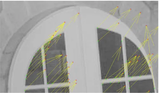
4.4 The detected feature points from the first and second frames of “garden.avi” by using the first scheme. The original gar-den sif.yuv sequence is taken from University of California Berkeley Multimedia Research Center. The green and red “+” signs are used for marking the locations of the feature points detected in the first frame and the second frame, respectively. . 61
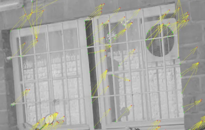
4.5 The assigned matches for the feature points from the first frame to second frame which are shown in Figure 4.4 by using the first scheme. The green and red “+” signs are used for marking the locations of the feature points detected in the first frame and the second frame, respectively. And the yellow arrows are showing the motion vectors. . . 62
4.6 A closer look at a set of matched points from the first frame to second frame which are shown in Figure 4.5 by using the first schemes. . . 63
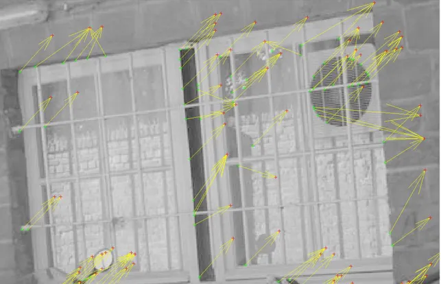
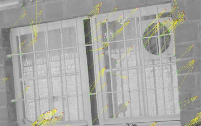
4.7 The detected feature points from the first and second frames of “garden.avi” by using the second scheme. . . 64
4.8 The assigned matches for the feature points from the first frame to second frame shown in Figure 4.7 by using the second scheme. 65
4.9 A closer look at a set of matched points from the first frame to second frame which are shown in Figure 4.5 by using the second scheme. . . 66
4.10 The detected feature points from the first and second frames of “garden.avi” by using the third scheme. . . 67
4.11 The assigned matches for the feature points from the first frame to second frame which are shown in Figure 4.10 by using the third scheme. . . 68
4.12 A closer look at a set of matched points from the first frame to second frame which are shown in Figure 4.5 by using the third scheme. . . 69
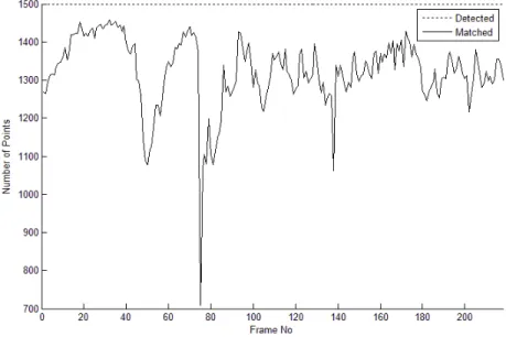
4.13 The detection and matching results of “garden.avi” for the first scheme. . . 70
4.14 The repetability and matching scores of “garden.avi” for the first scheme. . . 70
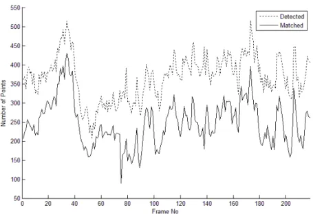
4.15 The detection and matching results of “garden.avi” for the sec-ond scheme. . . 71
4.16 The repetability and matching scores of “garden.avi” for the second scheme. . . 71
4.17 The detection and matching results of “garden.avi” for the third scheme. . . 72
4.18 The repetability and matching scores of “garden.avi” for the third scheme. . . 72
4.19 The difference between repetability score of 1st scheme and 2nd
or 3rd schemes for “garden.avi”. . . 73
4.20 The difference between match scores of 1st scheme and 2nd and
3rd schemes for “garden.avi”. . . 73
A.1 The detected feature points by using the Harris FPD. The orig-inal “bike” image couple is taken from Oxford University Visual Geometry Group. . . 106
A.2 The matched feature points among points detected shown in Figure A.1 by using gray-level patch description. The original “bike” image couple is taken from Oxford University Visual Ge-ometry Group. . . 107
A.3 The detected feature points by using the proposed FPD. . . 107
A.4 The matched feature points among points detected shown in Figure A.3 by using gray-level patch description. . . 108
A.5 The detected feature points by using the SIFT FPD. . . 108
A.6 The matched feature points among points detected shown in Figure A.5 by using gray-level patch description. . . 109
A.7 The detected feature points by using the proposed FPD with no scale selection. . . 110
A.8 The matched feature points among the detected points shown in Figure A.7 by using the proposed matching method. . . 111
A.9 The detected feature points by using the proposed FPD with the proposed scale selection. . . 112
A.10 The matched feature points among the detected points shown in Figure A.9 by using the proposed matching method. . . 113
A.11 The detected feature points by using the proposed FPD with the adjacent finer scale to the proposed scale is selected. . . 114
A.12 The matched feature points among the detected points shown in Figure A.11 by using the proposed matching method. . . 115
A.13 The detected feature points by using the proposed FPD with the adjacent coarser scale to the proposed scale is selected. . . . 116
A.14 The matched feature points among the detected points shown in Figure A.13 by using the proposed matching method. . . 117
B.1 The detection and matching results of “src6 ref 625.avi” for the first scheme. . . 119
B.2 The repetability and matching scores of “src6 ref 625.avi” for the first scheme. . . 119
B.3 The detection and matching results of “src6 ref 625.avi” for the second scheme. . . 120
B.4 The repetability and matching scores of “src6 ref 625.avi” for the second scheme. . . 120
B.5 The detection and matching results of “src6 ref 625.avi” for the third scheme. . . 121
B.6 The repetability and matching scores of “src6 ref 625.avi” for the third scheme. . . 121
B.7 The difference between repetability score of 1st scheme and
2ndor3rd schemes for “src6 ref 625.avi”. . . 122
B.8 The difference between match scores of 1st scheme and 2nd and
3rd schemes for “src6 ref 625.avi”. . . 122
B.9 The detection and matching results of “src10 ref 625.avi” for the first scheme. . . 123
B.10 The repetability and matching scores of “src10 ref 625.avi” for the first scheme. . . 123
B.11 The detection and matching results of “src10 ref 625.avi” for the second scheme. . . 124
B.12 The repetability and matching scores of “src10 ref 625.avi” for the second scheme. . . 124
B.13 The detection and matching results of “src10 ref 625.avi” for the third scheme. . . 125
B.14 The repetability and matching scores of “src10 ref 625.avi” for the third scheme. . . 125
B.15 The difference between repetability score of 1st scheme and 2nd
or 3rd schemes for “src10 ref 625.avi”. . . 126
B.16 The difference between match scores of 1st scheme and 2nd and
B.17 The detection and matching results of “src13 ref 525.avi” for the first scheme. . . 127
B.18 The repetability and matching scores of “src13 ref 525.avi” for the first scheme. . . 127
B.19 The detection and matching results of “src13 ref 525.avi” for the second scheme. . . 128
B.20 The repetability and matching scores of “src13 ref 525.avi” for the second scheme. . . 128
B.21 The detection and matching results of “src13 ref 525.avi” for the third scheme. . . 129
B.22 The repetability and matching scores of “src13 ref 525.avi” for the third scheme. . . 129
B.23 The difference between repetability score of 1st scheme and 2nd
or 3rd schemes for “src13 ref 525”. . . 130
B.24 The difference between match scores of 1st scheme and 2nd and
3rd schemes for “src13 ref 525”. . . 130
B.25 The detection and matching results of “src19 ref 525.avi” for the first scheme. . . 131
B.26 The repetability and matching scores of “src19 ref 525.avi” for the first scheme. . . 131
B.27 The detection and matching results of “src19 ref 525.avi” for the second scheme. . . 132
B.28 The repetability and matching scores of “src19 ref 525.avi” for the second scheme. . . 132
B.29 The detection and matching results of “src19 ref 525.avi” for the third scheme. . . 133
B.30 The repetability and matching scores of “src19 ref 525.avi” for the third scheme. . . 133
B.31 The difference between repetability score of 1st scheme and 2nd
or 3rd schemes for “src19 ref 525”. . . 134
B.32 The difference between match scores of 1st scheme and 2nd and
3rd schemes for “src19 ref 525”. . . 134
B.33 The detection and matching results of “src20 ref 525.avi” for the first scheme. . . 135
B.34 The repetability and matching scores of “src20 ref 525.avi” for the first scheme. . . 135
B.35 The detection and matching results of “src20 ref 525.avi” for the second scheme. . . 136
B.36 The repetability and matching scores of “src20 ref 525.avi” for the second scheme. . . 136
B.37 The detection and matching results of “src20 ref 525.avi” for the third scheme. . . 137
B.38 The repetability and matching scores of “src20 ref 525.avi” for the third scheme. . . 137
B.39 The difference between repetability score of 1st scheme and 2nd
or 3rd schemes for “src20 ref 525”. . . 138
B.40 The difference between match scores of 1st scheme and 2nd and
B.41 The detection and matching results of “src22 ref 525.avi” for the first scheme. . . 139
B.42 The repetability and matching scores of “src22 ref 525.avi” for the first scheme. . . 139
B.43 The detection and matching results of “src22 ref 525.avi” for the second scheme. . . 140
B.44 The repetability and matching scores of “src22 ref 525.avi” for the second scheme. . . 140
B.45 The detection and matching results of “src22 ref 525.avi” for the third scheme. . . 141
B.46 The repetability and matching scores of “src22 ref 525.avi” for the third scheme. . . 141
B.47 The difference between repetability score of 1st scheme and 2nd
or 3rd schemes for “src22 ref 525”. . . 142
B.48 The difference between match scores of 1st scheme and 2nd and
3rd schemes for “src22 ref 525”. . . 142
B.49 The detection and matching results of “whaleshark planetEarth eps11.avi” for the first scheme. . . 143
B.50 The repetability and matching scores of “whaleshark planetEarth eps11.avi” for the first scheme. . . 143
B.51 The detection and matching results of “whaleshark planetEarth eps11.avi” for the second scheme. . . 144
B.52 The repetability and matching scores of “whaleshark planetEarth eps11.avi” for the second scheme. . . 144
B.53 The detection and matching results of “whaleshark planetEarth eps11.avi” for the third scheme. . . 145
B.54 The repetability and matching scores of “whaleshark planetEarth eps11.avi” for the third scheme. . . 145
B.55 The difference between repetability score of 1st scheme and 2nd
or 3rd schemes for “whaleshark planetEarth eps11.avi”. . . 146
B.56 The difference between match scores of 1st scheme and 2nd and
3rd schemes for “whaleshark planetEarth eps11.avi”. . . 146
B.57 The detection and matching results of ‘goats planetEarth eps5.avi” for the first scheme. . . 147
B.58 The repetability and matching scores of “goats planetEarth eps5.avi” for the first scheme. . . 147
B.59 The detection and matching results of “goats planetEarth eps5.avi” for the second scheme. . . 148
B.60 The repetability and matching scores of “goats planetEarth eps5.avi” for the second scheme. . . 148
B.61 The detection and matching results of “goats planetEarth eps5.avi” for the third scheme. . . 149
B.62 The repetability and matching scores of “goats planetEarth eps5.avi” for the third scheme. . . 149
B.63 The difference between repetability score of 1st scheme and 2nd
or 3rd schemes for “goats planetEarth eps5.avi”. . . 150
B.64 The difference between match scores of 1st scheme and 2nd and
B.65 The detection and matching results of “dolphins planetEarth eps9.avi” for the first scheme. . . 151
B.66 The repetability and matching scores of “dolphins planetEarth eps9.avi” for the first scheme. . . 151
B.67 The detection and matching results of “dolphins planetEarth eps9.avi” for the second scheme. . . 152
B.68 The repetability and matching scores of “dolphins planetEarth eps9.avi” for the second scheme. . . 152
B.69 The detection and matching results of “dolphins planetEarth eps9.avi” for the third scheme. . . 153
B.70 The repetability and matching scores of “dolphins planetEarth eps9.avi” for the third scheme. . . 153
B.71 The difference between repetability score of 1st scheme and 2nd
or 3rd schemes for “dolphins planetEarth eps9.avi”. . . 154
B.72 The difference between match scores of 1st scheme and 2nd and
3rd schemes for “dolphins planetEarth eps9.avi”. . . 154
B.73 The detection and matching results of “leopard planetEarth eps2.avi” for the first scheme. . . 155
B.74 The repetability and matching scores of “leopard planetEarth eps2.avi” for the first scheme. . . 155
B.75 The detection and matching results of “leopard planetEarth eps2.avi” for the second scheme. . . 156
B.76 The repetability and matching scores of “leopard planetEarth eps2.avi” for the second scheme. . . 156
B.77 The detection and matching results of “leopard planetEarth eps2.avi” for the third scheme. . . 157
B.78 The repetability and matching scores of “leopard planetEarth eps2.avi” for the third scheme. . . 157
B.79 The difference between repetability score of 1st scheme and 2nd
or 3rd schemes for “leopard planetEarth eps2.avi”. . . 158
B.80 The difference between match scores of 1st scheme and 2nd and
3rd schemes for “leopard planetEarth eps2.avi”. . . 158
B.81 The detection and matching results of “container.avi” for the first scheme. . . 159
B.82 The repetability and matching scores of “container.avi” for the first scheme. . . 159
B.83 The detection and matching results of “container.avi” for the second scheme. . . 160
B.84 The repetability and matching scores of “container.avi” for the second scheme. . . 160
B.85 The detection and matching results of “container.avi” for the third scheme. . . 161
B.86 The repetability and matching scores of “container.avi” for the third scheme. . . 161
B.87 The difference between repetability score of 1st scheme and 2nd
or 3rd schemes for “container.avi”. . . 162
B.88 The difference between match scores of 1st scheme and 2nd and
B.89 The detection and matching results of “coastguard.avi” for the first scheme. . . 163
B.90 The repetability and matching scores of “coastguard.avi” for the first scheme. . . 163
B.91 The detection and matching results of “coastguard.avi” for the second scheme. . . 164
B.92 The repetability and matching scores of “coastguard.avi” for the second scheme. . . 164
B.93 The detection and matching results of “coastguard.avi” for the third scheme. . . 165
B.94 The repetability and matching scores of “coastguard.avi” for the third scheme. . . 165
B.95 The difference between repetability score of 1st scheme and 2nd
or 3rd schemes for “coastguard.avi”. . . 166
B.96 The difference between match scores of 1st scheme and 2nd and
3rd schemes for “coastguard.avi”. . . 166
B.97 The detection and matching results of “foreman.avi” for the first scheme. . . 167
B.98 The repetability and matching scores of “foreman.avi” for the first scheme. . . 167
B.99 The detection and matching results of “foreman.avi” for the second scheme. . . 168
B.100The repetability and matching scores of “foreman.avi” for the second scheme. . . 168
B.101The detection and matching results of “foreman.avi” for the third scheme. . . 169
B.102The repetability and matching scores of “foreman.avi” for the third scheme. . . 169
B.103The difference between repetability score of 1st scheme and 2nd
or 3rd schemes for “foreman.avi”. . . 170
B.104The difference between match scores of 1st scheme and 2nd and
3rd schemes for “foreman.avi”. . . 170
B.105The detection and matching results of “janine1 1.avi and ja-nine1 2.avi” for the first scheme. . . 171
B.106The repetability and matching scores of “janine1 1.avi and ja-nine1 2.avi” for the first scheme. . . 171
B.107The detection and matching results of “janine1 1.avi and ja-nine1 2.avi” for the second scheme. . . 172
B.108The repetability and matching scores of “janine1 1.avi and ja-nine1 2.avi” for the second scheme. . . 172
B.109The detection and matching results of “janine1 1.avi and ja-nine1 2.avi” for the third scheme. . . 173
B.110The repetability and matching scores of “janine1 1.avi and ja-nine1 2.avi” for the third scheme. . . 173
B.111The difference between repetability score of 1st scheme and 2nd
or 3rd schemes for “janine1 1.avi and janine1 2.avi”. . . 174
B.112The difference between match scores of 1st scheme and 2nd and
B.113The detection and matching results of “jungle 1.avi and jun-gle 2.avi” for the first scheme. . . 175
B.114The repetability and matching scores of “jungle 1.avi and jun-gle 2.avi” for the first scheme. . . 175
B.115The detection and matching results of “jungle 1.avi and jun-gle 2.avi” for the second scheme. . . 176
B.116The repetability and matching scores of “jungle 1.avi and jun-gle 2.avi” for the second scheme. . . 176
B.117The detection and matching results of “jungle 1.avi and jun-gle 2.avi” for the third scheme. . . 177
B.118The repetability and matching scores of “jungle 1.avi and jun-gle 2.avi” for the third scheme. . . 177
B.119The difference between repetability score of 1st scheme and 2nd
or 3rd schemes for “jungle 1.avi and jungle 2.avi”. . . 178
B.120The difference between match scores of 1st scheme and 2nd and
3rd schemes for “jungle 1.avi and jungle 2.avi”. . . 178
B.121The detection and matching results of “cam0 capture5 Deniz.avi and cam1 capture5 Deniz.avi” for the first scheme. . . 179
B.122The repetability and matching scores of “cam0 capture5 Deniz.avi and cam1 capture5 Deniz.avi” for the first scheme. . . 179
B.123The detection and matching results of “cam0 capture5 Deniz.avi and cam1 capture5 Deniz.avi” for the second scheme. . . 180
B.124The repetability and matching scores of “cam0 capture5 Deniz.avi and cam1 capture5 Deniz.avi” for the second scheme. . . 180
B.125The detection and matching results of “cam0 capture5 Deniz.avi and cam1 capture5 Deniz.avi” for the third scheme. . . 181
B.126The repetability and matching scores of “cam0 capture5 Deniz.avi and cam1 capture5 Deniz.avi” for the third scheme. . . 181
B.127The difference between repetability score of 1st scheme
and 2nd or 3rd schemes for “cam0 capture5 Deniz.avi and
cam1 capture5 Deniz.avi”. . . 182
B.128The difference between match scores of 1st scheme and
2nd and 3rd schemes for “cam0 capture5 Deniz.avi and
cam1 capture5 Deniz.avi”. . . 182
B.129The detection and matching results of “cam0 capture7 novice jugglers.avi and cam1 capture7 novice jugglers.avi” for the first scheme. . . 183
B.130The repetability and matching scores of “cam0 capture7 novice jugglers.avi and cam1 capture7 novice jugglers.avi” for the first scheme. . . 183
B.131The detection and matching results of “cam0 capture7 novice jugglers.avi and cam1 capture7 novice jugglers.avi” for the second scheme. . 184
B.132The repetability and matching scores of “cam0 capture7 novice jugglers.avi and cam1 capture7 novice jugglers.avi” for the second scheme. . 184
B.133The detection and matching results of “cam0 capture7 novice jugglers.avi and cam1 capture7 novice jugglers.avi” for the third scheme. . . 185
B.134The repetability and matching scores of “cam0 capture7 novice jugglers.avi and cam1 capture7 novice jugglers.avi” for the third scheme. . . 185
B.135The difference between repetability score of 1st scheme and
2nd or 3rd schemes for “cam0 capture7 novice jugglers.avi and
cam1 capture7 novice jugglers.avi”. . . 186
B.136The difference between match scores of 1st scheme and 2nd
and 3rd schemes for “cam0 capture7 novice jugglers.avi and
List of Tables
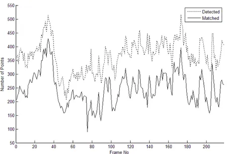
4.1 The number of detected and matched points and the match and repetition scores of the Harris, proposed and SIFT detectors for the test image couples. . . 48
4.2 The number of detected and matched points and the match and repetition scores of the Harris FPD for the test image couples. . 49
4.3 The number of detected and matched points and the match and repetition scores of the Gray-level patch, proposed and SIFT descriptors for the test image couples. . . 51
4.4 The number of detected and matched points and the match and repetition scores of the SIFT descriptors for the test image couples 52
4.5 The number of detected and matched points and the match and repetition scores of different scale selection schemes for the test image couples. . . 54
4.6 The number of following, not following, correct matches and wrong matches for the image patch given in Figure 4.3. . . 55
4.7 The properties of video sequences. . . 57
Chapter 1
Introduction
Feature point detection is one of the vital topics in image processing. Ad-vancements in feature point detection techniques directly affect many open to research areas such as 3D scene reconstruction, object recognition, image reg-istration, etc. Though the literature on feature point detection can be dated back to the late 70’s, there is still no universal feature point detector. Currently the most widely used detector was designed in the late 80’s. It has evolved since then but it is still far from an ideal universal feature point detector.
1.1
Feature Point Detection Concepts
A feature point is a salient point, which can be easily separated from the surrounding pixels. The most intuitive feature (or salient) points are corners in an image. There have been many different detectors to accurately localize such points. They can be initially separated into two groups: the detectors which operate on black and white edge contours, and, the ones which operate on gray-level images. We can also include the detectors which operate on color images but these detectors are essentially extensions of their gray-level
counterparts. As a result, color image detectors are not counted as a separate class.
After broadly categorizing the feature point detection algorithms, we are going to introduce the detectors which are the milestones of the feature point detection literature. During the introduction we are going to explain some of the detectors in more detail. We begin with the gray-level feature point detectors.
An early feature point detector in this class was designed by Moravec to detect corners[14]. The detector basically measures the directional variance around a pixel. To measure the directional variance, correlations in the neigh-boring blocks around pixels are computed. By doing this directional derivatives around pixels are implicitly measured. As a result, this detector is known as the first derivative-based feature point detector or “interest point detector” as Moravec named it.
The Moravec’s detector was followed by Kitchen and Rosenfeld’s detector [15]. They noticed that corners lay along edge intersections. They proposed that the corner detection accuracy might increase if the edges in the image were detected and used for eliminating non-corner points. To implement the detector, they combined a directional derivative based detector with an edge detector. The corner detection performance was increased as a result of this restriction.
The Moravec’s detector had a serious drawback; the detector was limited by a small number of derivative directions. Moravec used 45 degrees shifted windows in the estimation of the correlation. This shifting scheme limits the derivative directionality. As a result, Moravec’s detector misses arbitrarily aligned corners. In the late 80’s Harris and Stephens analytically solved the problem of direction limitation and modified the Moravec’s detector. In their
paper [16], Harris and Stephens showed that there was a strict relation be-tween directional variance measure and local autocorrelation of an image patch. Moreover, they also proved that by using the gradients of an image, local auto-correlation function can be approximated for small shifts, instead of 45 degree shifts. Besides, they also showed that the gradient of an image, that can be used in approximation of the local autocorrelation function, could be estimated from both vertical and horizontal first-degree partial derivatives. With all of these observations and approximations, they estimated the directional vari-ance measure and the local autocorrelation function for small shifts according to: E(x, y) = [x y]M[x y]t, (1.1) M = A C C B ; A = (∂I ∂x) 2, B = (∂I ∂y) 2, C = ∂I ∂x ∂I ∂y. (1.2)
In the equations x and y represent image coordinates, M represents the Hes-sian matrix, E represents cumulative directional variance and I represents the image intensity. The details about the variables and derivations can be found in [16].
Due to practical reasons, they used the matrix M to find corners, instead of using E(x, y). The eigenvalues (a, b) of M are proportional to the principle curvature of the local autocorrelation function. The principle curvature and, indirectly, the eigenvalues of M, define whether a pixel is on a flat region, edge or corner. Nevertheless, due to the difficulties in computation of eigenvalues, the determinant and trace of M are used in the computation of the cornerness function R, where
R = det(M) − k × T r(M), det(M) = AB − C2, T r(M) = A + B. (1.3)
In this equation det(M) and T r(M) are determinant and trace of matrix M, respectively; k is a constant which depends on various properties of image such
for each pixel of an image. Then the local maxima, which are greater than a positive threshold, are chosen as corners.
Due to the analytical and computational limitations, as previously ex-plained, they left the detector incomplete. Three years after Harris and Stephens published the detector, Tomasi and Kanade finished the incomplete work [17]. In the Harris corner detector eigenvalues were not computed due to computational complexity and reliability. However, in the gradient-based corner detection, the eigenvalues of the Hessian matrix give the most impor-tant cues about the cornerness of a pixel. So, in the Tomasi-Kanade corner detector, primarily, the Harris corner detector is applied to the image in order to reduce the computational load. Then, for each candidate corner, the eigen-values of the matrix M are computed. After that a histogram is generated from the minimum of the eigenvalue pairs. Consequently, the histogram is examined for a breaking point. The breaking point defines the threshold for candidate pixels elimination. The detector selects the pixels with the minor eigenvalue greater than the threshold and sorts them in decreasing order. The sorting is very important because when the minimum eigenvalue is higher, the pixel becomes more reliable. Hence, matching starts from the top of the sorted corner list.
The detectors explained above use partial derivatives or derivative approx-imations to calculate surface curvature of the gray-level images. It should be noted that there are also other algorithms which use similar techniques to solve the feature point detection problem, given in [18], [19], [20], [21], [22], [23], [24].
In the mid 90’s Lindeberg introduced a semi-automatic derivative-based multi-resolution feature point detection algorithm [27]. Mainly the detector creates a Gaussian pyramid from an image. Then it chooses points which are maximum along the scale direction. With this detection scheme one can not only detect a feature point but also select a validity scale in which matching
should be done. This was one of the leading multi-resolution feature point detection schemes and inspired many researchers.
In the early 2000, Scale Invariant Feature Transform (SIFT), another resolution feature point detector, was introduced by Lowe[25]. SIFT is a multi-scale feature point detection scheme. In SIFT, all of the multi-scales are searched to find the interest points which are both spatial and scale local extrema.
The method starts with creating a form of space. The SIFT’s scale-space is produced from octaves. Octave intervals are either half or double of the previous or next octave, respectively. Octaves are generated by convolving the original image with a Gaussian Kernel (or basis). Each octave interval is divided into “s” many scales by convolving with another Gaussian kernel, but scales are not downsampled after the convolution. All of the images in an oc-tave interval have the same resolution. Images are downsampled when moving from one octave to a lower one. After the scale-space is created, the adjacent scales in an octave are subtracted from each other to form the difference of Gaussian image. After that the feature points are detected by comparing the points with their spatial and scale neighbors. The points, which are local ex-trema in both scale and space, are selected as feature points. To accurately localize feature points a 3D quadratic function is fitted to the neighborhood of the detected corners. The quadratic function also helps to achieve subpixel resolution.
After the SIFT detector another multi-resolution feature point detector, Harris-Laplacian corner detector, was introduced by Mikolajczyk et.al [26]. The Harris-Laplacian corner detector treats values of each pixel locations on an image as a 1D signal in the scale dimension. Initially, Harris-Laplacian feature point detector detects corners by using Harris corner detector. Then, scale properties of each corner are determined by convolving each scale with a specific function and investigating 1D response with respect to scale as shown
in Figure 1.1. Then the scale that the maximum of 1D signal occurred is selected as the characteristic scale, which is used for setting a common scale between the different views of the same scene as Lindeberg showed in [27]. At the end, corners and their characteristic scales, in which the feature point is valid, are determined. In this method, both Harris detector and Laplacian function are used since they are the optimal operators for the specified cases according to the experiments in the paper by Mikolajczyk et.al [26].
Figure 1.1: Selection of the characteristic scale
Morphological operators are also one of the important tools in signal pro-cessing. Various morphological detectors were proposed for feature point de-tection [28], [29], [30], [31], [32]. Main advantage of these detectors is the low computation load which allows real-time operations.
Some transformation based methods were also proposed. Basically, trans-formations represent the image data in a simpler and/or more useful way which makes the detection process easier (and faster). Various different trans-formations are used for feature point detection, such as Hilbert transform [40], wavelet transform [41], [42], matched filtering [43], various filter banks [44], and the phase congruency [38], [39], etc. Each of these detectors have different properties.
Finally, there are also some custom detectors which are applied to gray-level images. Some of these are based on non-linear operators [36], [37], some assigns cost functions to each pixel and minimizes it [35], some uses proba-bilistic models to detect corners [23] and some of them uses models to detect corners [33], [34].
Boundary based feature point detection is analogous to the gray-level de-tection. For example, derivative based techniques, as in the gray-level case, were proposed to detect the curvature of the contour (or edge) [1], [2], [3], [4], [5]. Transform based boundary techniques were also proposed in [7], [13]. Also custom boundary methods were proposed using various techniques, such as neural-networks to estimate curvature [6], correlation or L2norm to find
sim-ilarity [1], [11], chain codes to simplify the representation [8], [9], covariance metrics along the contour [10] and probabilistic approaches [12].
1.2
Problem Statement
As shown in the previous section, the aim of the most widely used feature detection algorithms is to detect corners. This approach leads to many prob-lems as shown in various comparisons [45],[46]. The origin of the probprob-lems is that there is no robust definition of the corner concept. And some of the non-corner points also satisfy the existing non-cornerness criteria. Moreover, real-life cases make it even harder. For example, in Figure 1.2 we can see that due to downsampling, misleading corner structures are formed and these causes detectors to extract non-corner points as corners, even without aliasing effect during downsampling. This figure also shows us that the number of corners changes with respect to resolution. For example, when the detector is applied to a finer resolution image and its coarser resolution image, most of the cor-ners, detected in the finer resolution, are lost in the coarser resolution due to the filtering which is used to avoid aliasing after downsampling.
Another problem with the many detectors is they use derivative based methods which are inherently erroneous in noisy environments. Moreover, when quantization is added to this situation, extracting corners accurately becomes a difficult task. Furthermore, in images, there are many non-corner
Figure 1.2: A corner sample with zoom-in
pixels which satisfies the multiple high directional derivative test, which is standard in derivative based detectors.
In addition to these drawbacks, the corner detectors have a lot of param-eters which vary from one image to another. Most of the detectors even do not have an automatic parameter selection scheme. As each of the parame-ters change independently according to image properties, such as contrast, the manual detectors become hard to use. Because, to reduce possible errors the user should adjust the parameters for every different case, which significantly changes in real life situations.
The fundamental assumption of most of the feature point detectors, explic-itly or implicexplic-itly, is “objects in images can be expressed as edges or contours”. To have this representation, first of all edges (or contours) in images should be detected. The edges were assumed to represent the object boundaries. And irregularities on the boundaries are used as feature points, because they store more information than others. This basic assumption can be seen clearly in different detectors which operate on contours. However, it is not that obvious in detectors which operate on gray-level images. This is because edge detectors are combined with corner detectors. This can be seen in many algorithms such as [15], [16], [18], [25], [26], [36], etc. There are also some custom detectors which do not integrate an edge detector. But these detectors are also searching for a corner instead of a feature point. So, that custom detectors suffer from almost the same drawbacks as the other ones.
However, as shown in [25], [26], these drawbacks can be lessen by applying multi-resolution analysis in gradient estimation. Moreover, by describing fea-ture points according to deviations around them and not by gray-level patches, SIFT detection-matching scheme has improved its performace more than the others. Hence, the algorithms are stablized and gained immunity to various real-life cases which cause to detection of non-feature point.
Due to these reasons, we propose a post-processing scheme to reduce the number of detected non-corner points. In this approach it is believed that objects in images should be represented by regions instead of edges/contours and each one of the feature points should be represented with respect to its neighborhood. Therefore, we can measure the degree of distinctiveness of a detected feature point among its neighbors. By using this measure non-feature points can be eliminated.
Moreover, we can also use this neighborhood description in feature point matching. A feature point is not an isolated pixel; due to physical constraints, it closely depends on its neighborhood. Therefore, if we use neighborhood conditioned pixel description, we can improve the matching quality.
The proposed post-processing and matching scheme should have some es-sential properties. For example, the method should be easily implementable and robust under mostly unpredictable, real-life cases. Therefore, the aim of the thesis is to design and implement a post-processing and matching method which is implementable and robust as explained previously, and increases the performance of applications which rely on feature point detection.
In order to have the proposed post-processing and matching scheme, we need to understand the properties of textures. Because, when we are referring to describe a point with respect to its neighbors; we are implicitly representing
the texture around a feature point. This is, in fact, one of the crucial steps in our proposed post-processing and matching scheme.
Chapter 2
Texture
Although textures can be easily perceived and distinguished by humans, there is no single definition of texture. For example in analysis sense, we can think of a texture as a region which is homogeneous in some extent. However, the definition of the homogeneity depends on texture and observer. In the synthesis sense, we can think of a texture as an output of a process. Nevertheless, the texture generating process is, in most cases, highly complex and unknown. In almost every situation, the bottleneck of texture studies is the lack of a single definition.
2.1
Texture Definition
As previously mentioned there is no single texture definition and tens of dif-ferent definitions can be found in the literature. However, there are two basic definitions given by Sklansky et.al [56] and Tamura [55]. These definitions are essential to understand the texture concept.
Texture, according to Sklansky, is a regional attribute whose local proper-ties (statistics) are constant, slowly varying or almost periodic.
On the other hand, texture, according to Tamura, can be expressed by a number of primitives which have various spatial organizations.
We can think the second definition and its variants as a subset of the first one. Because, if we know the repeating primitive, we can extract its statistical attributes and use these to define a homogeneity measure. The homogeneity measure helps to indicate whether a region is locally constant, slowly varying or periodic as stated in the first definition.
As the first definition covers most of the others definitions, we are going to use the first definition which is moderately broad, when compared with the others which are given in [173]. Hence, to be more precise, “texture” term is used to describe a region which is composed of closely blended or mixed elements with properties defined by Sklansky et.al [56].
In order to use this definition in a specific case, we have to extract ho-mogeneity measure (statistical attributes) of the texture by applying texture analysis methods.
2.2
Texture Analysis
In this section, we are going to overview not only texture analysis, but also synthesis and segmentation methods. Because, almost all of the analysis, syn-thesis and segmentation algorithms rely on similar fundamental assumptions. And as a result, almost all of the texture processing methods (analysis, syn-thesis and segmentation) give insight about textures and performance of the applied methods.
One of the earliest methods was proposed by Haralick et.al. [57] in 1973. The proposed method was based on second order statistics or in other words “occurrence frequencies” [67], [66] . Basically, they generate a square matrix
for a specific separation distance and angle. This separation distance and angle define the distance between the reference pixel and the pixels under investigation. The row and column indices of the matrix represent the gray-level of the current pixel and the pixels under examination, respectively. As a result, the matrix represents the occurrence frequencies of gray-levels pairs at the given separation distance. This matrix form is also known as “co-occurrence matrix”. A simple co-“co-occurrence matrix (Pd,angle) for a binary
image is given by Pd,angle = pi,j pi+1,j pi,j+1 pi+1,j+1 ; i = 0, j = 0. (2.1)
Note that, pi,j denotes the occurrence frequency of a pixel which has value
i, separated from another pixel which has value j, with a specific distance d and angle. Furthermore, to analyze the given texture, many matrices are
computed for different angles and separations [58].
The computational load of co-occurrence matrix can be reasonable for a binary image, but it becomes relatively too large to be used alone, when the number of quantization levels increases. As a result, various different features were defined to represent co-occurrence matrices in simpler forms [60], [64], [65]. Furthermore, the description performance was improved by applying DCT to the co-occurrence matrices to make the components less correlated [63]. What is more important, several fast co-occurrence matrix computation methods were proposed [61], [62].
Nevertheless, as most of the other texture analysis methods, this technique suffers from a huge computational load. As the aim was extracting second order statistics, the computation load increases exponentially with the increasing
from a binary image has two dimensions and four elements. On the other hand, a co-occurrence matrix generated from an 8-bit gray-level image has 256 dimensions and 65536 elements and that causes a fairly high computation cost for a single pixel.
Another early approach was based on autoregressive image models. In this approach, autoregressive models (AR) were used to extract the underlying texture statistics [68]. Basically, AR models are used in predicting the future values of time-series as:
Xt= c + p
X
i=1
φiXt−i+ ²t. (2.2)
where Xtis the value to be predicted, Xt−i are the past values, p is the order of
the prediction, ²t is the prediction error and φi are the prediction coefficients.
As can be seen in the equation, AR models also emphasize the short-range interaction by weighting past values. The weighting is used to define statistical properties of textures.
In image processing, time-series are formed from images in a raster-scan scheme. In the raster-scan, images are transformed from N × N matrices to
N2× 1 vectors. As a result, a series is formed from an image which has some
basic properties like causality.
There are many different autoregressive models. The main goal of AR methods is finding the best model to represent a given texture. Various AR models were proposed, such as, non-causal AR [69], [76], simultaneous AR [70], [72], [71], multiresolution Gaussian AR [73], circular symmetric AR [74], 2D quarter-plane AR [75], recursive AR [77], generalized circular AR [78], etc.
According to the applied model, prediction coefficients are computed. And based on the coefficients, texture statistics are defined. Abbadeni [79] gives some examples on AR model parameters and their perceptual meaning.
AR models have proved their usefulness in extracting the underlying sta-tistical behavior of time-series. There are many well-known signal processing algorithms which use these models, such as GSM vocoders. Furthermore, with some improvements, such as making them rotation and scale invariant, they become a good texture descriptor.
Another model-based approach is based on Markov (or Gibbs) random fields. Briefly, Markov (or Gibbs) random field (M/GRF) approaches interpret images as random fields. In a Markov/Gibbs random field, the probability of the value of a pixel depends only on the values of the neighboring pixels. This is known as the Markovian property. And the conditional probability distribution function, which is occurrence of a pixel conditioned to its neighborhood, is in exponential form. Further information on M/GRFs can be found in [98] and [97].
Although the M/GRF model and its multi-resolution counterparts, [96], [87], [93], [89], are well-defined and straightforward, estimation of the model parameters is tricky. Moreover, instead of the others, proposed approaches vary in parameter estimation algorithms. For instance, some approaches use dynamic programming [81], [91], [82], [83]; some use pseudo-maximum likeli-hood [86]; instead of maximum likelilikeli-hood, some use least squares [84] whereas some others use simulated annealing [85], [80], [94] and [90].
In each of the proposed methods there is a trade-off between computational complexity and parameter estimation accuracy. For example, the parameters can be estimated accurately by using simulated annealing (SA) but the compu-tation load of SA can be overwhelming. On the other hand, the compucompu-tational load may be low if the least squares estimation methods are used. However, the estimation accuracy will be poorer in this case.
Another well-known model based texture analysis method was proposed by Pentland et.al.[99]. In that paper, the textures are modelled as fractal func-tions. Fractals are described by their complexity. The complexity parameter is known as “fractal dimension”. As in the parameter estimation of M/GRF model, estimating the fractal dimension is difficult. Many different ways to es-timate the fractal dimension were proposed, [102], [103], [104]. Though some of them are useful, it was shown that fractal dimensions alone cannot be used to discriminate different textures [106]. To overcome the lack of discrimination, some modifications were suggested, such as using lacunarity measures [105], [100], extended self-similarity model [101], etc.
Transformation techniques are highly important in signal processing. Ba-sically, transforming a signal from one space to another, where they can be represented according to the needs, has positive effects on performance; such as, increasing accuracy, decreasing computation load, etc. As in the other sig-nal asig-nalysis cases, sigsig-nal transformation techniques can be helpful in texture analysis, too. Because, based on experiments, each texture has a specific sig-nature and transforms can be used to represent textures in a more useful form to easily extract these signatures. Therefore, the purpose of the transform based methods is representing a texture in an appropriate way and finding its characteristic signatures. We have to mention here that these signatures are not unique for every texture. Because, in addition to these structural signa-tures, textures also have a random characteristic. Nevertheless, extraction of these signatures are generally enough for most cases.
In order to extract the texture signatures, Short Time Fourier Transform is used in [107], [108], [109]. In [110], [111] the Circular-Mellin Transform, which is Fourier Transform in polar coordinates, is used to extract scale-rotation in-variant features from textures. Furthermore, also Gabor Transform is utilized in various approaches. Some of the approaches create a filter bank which covers
large portion of the space-spatial frequency domain [127], [128], [129], [132], [133], [134], [137] and [138]. Some of them propose adaptive filter parameter (center frequency, orientation, bandwidth) selection schemes for the given in-put textures [139], [131], [135] and [136]. Moreover, Wigner Ville Distribition based methods were also applied in texture analysis in different ways by [117], [118] and [119].
Another integral transform texture analysis method is called “Local Linear Transform” (LLT). In LLT, the texture is convolved by a custom filter bank. Then, the energy of the channels (filter outputs) are used in feature selection. Various methods were proposed [151], [152], [153], [154], [155], [156], [157], [158], [159], [161] and [160]. One of the famous LLT was proposed by Laws who uses wavelet like basis [159]. The performance of LLT can be improved by using DCT to decorrelate the filter output [153].
There are also some custom texture analysis methods. These methods use various techniques, such as moments [162], [163], [164], histograms [174], metric spaces[175], run-lengths[176], Voronoi polygons[177], dynamic matched filtering [179], local frequency[180], etc.
Chapter 3
Non-Feature Point Elimination
And Feature Point Matching
Images and video frames can be used for different purposes and objectives. In some applications, such as 3D scene reconstruction, object recognition, image registration, etc., one may want to uncover point-to-point relations between two images (or frames). There are various ways to find out this relation. One of the popular ways of this is finding matches between the images (or frames). In this type of methods points are represented by some attributes. And the point on the other image with the most similar attributes are assigned as a match. The operation of making point-to-point similarity assignments is known as “Point Matching”.
To make better matches between images (or frames) instead of ordinary points, the points with some distinctive features are selected. And the match-ing is started from these points. The operation of selectmatch-ing distinctive points is known as “Feature Point Detection”. However, the selection of distinctive points is complicated. Images contain variety of pixel combinations and these
combinations sometimes fulfill the feature point criteria of detectors and de-ceive the detection algorithms. As a result of this, the set of detected points contains both feature points and non-feature points.
The false selection of a non-feature point as a feature point is highly un-desirable. The inclusion of these points in a set of feature points decreases the reliability of matching step. Because, as these points are not distinctive enough, they may cause mismatches. Due to the inadequate matchings, most of the applications which rely on point-to-point matches may give erroneous and unpredictable results. Hence, to ensure the performance of the applica-tions which rely on feature matching non-feature point should be eliminated.
However, the methods used in detection may not solve the elimination problem, because, non-feature points may have higher detection scores than regular feature points. As a result of this some desired feature points may be discarded while trying to eliminate non-feature points by using the approaches similar to the detection methods. Due to this, a different approach should be utilized in elimination.
As explained in the first chapter, most of the popular feature point detec-tion methods directly or indirectly uses color or intensity attributes of pixels to describe them. However, just color or intensity values are not enough to rep-resent the distinctiveness of a pixel. There should be additional or alternate, descriptors to represent the pixel attributes.
Describing the texture around a point is one of the important elements for representing regional attributes of a point. As explained in chapter 2 there are various ways of describing a texture, basically each of these descriptors uses the neighborhood structure around a pixel to form a regional point represen-tation. As feature points should be distinctive among their neighbors, texture based descriptions are highly useful in pixel classification. Furthermore, these
descriptors can also be used in feature matching, too; because, due to physi-cal constraints neighborhoods may preserve their structure. Hence, for every candidate point couple both pixel-wise and regional attributes should match each other. Due to this, better matching results can be obtained by including texture descriptors in point representation.
Although texture description is one of the powerful tools in image process-ing, it creates some undesired complications in implementation. First of all creating a texture description around each of the pixels of an image is compu-tationally impractical. Because, it requires a large memory space and a high processing power. Even applying texture description only to a set of feature points is computationally overwhelming, due to the scale dependency of tex-tures. Nevertheless, there are ways to bypass these implementation problems.
3.1
Scale Selection
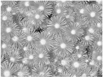
Images can be represented in different ways, one of them is representing images in multi-resolution. In multi-resolution, an image with spatial resolution N ×M per unit area is filtered and downsampled by d to have a coarser image with smaller resolution N/d×M/d per unit area. The acquired image representation is called a scale. An image and its two scales are given in Figure 3.1 and Figure 3.2, respectively.
The collection of extracted scales is called the “scale-space”. In the pro-posed method the coarsest and the finest scales of a scale-space is restricted. The range of scales are limited between the sampling rate of the imaging sensor (finest resolution) and a single pixel (coarsest resolution).
Infinitely many scales, in a given range, can be extracted from an image. Furthermore, each of the patches extracted from different scales at relatively
Figure 3.1: A scale of a sample image with textures
Figure 3.2: Another scale of the same image shown in Figure 3.1
on the same position may have different pixel values. As pixel values inside the patches change from one scale to another, neighborhood structure also changes. Hence, the nature of the texture changes. In order to have a complete texture description every scale of an image should be analyzed and represented.
This scale dependency of textures creates a serious bottleneck in implemen-tation, even for the proposed elimination method which processes relatively a small number of points. One of the solutions to this computation problem is choosing a single scale for analysis according to texture signatures and ignoring the rest of the scale-space.
As explained in the second chapter, every texture has a signature in the scale-space. In the scale selection, the scale which contains the most discrimi-native texture signatures is desired. Because, if the selected analysis scale does
not supply discriminative information, then the extracted texture description will be misleading. And, at the end, the entire approach will be useless.
For example, in the Gabor filter bank case, if one of the filters is tuned to a range which is out of the scale in which the discriminative texture sig-nature lies, then the resultant description may have noise like terms which may give misleading information about the content. This observation also holds for Gibbs/Markov random fields. Basically, GMRF describes a texture by clique potentials which represent pixelwise interactions. These interactions are derived from pixel formations. As pixel formations depend on scale, GMRF structure and model parameters change, too. Hence, if nondiscriminative pixel interactions are modeled, texture may be represented in a misleading way. And the descriptor will be ineffective.
To have an adequate texture description, first of all, a color space should be selected. There are various ways to use a spectral image in multi-resolution analysis. In the proposed method the luminance channel of
CIE L∗a∗b∗ color space is used [189]. The given image, generally in RGB
24-bit raw format, is transform to CIE L∗a∗b∗ color space based on ITU-R
BT.709 using D65 as the white point reference [191]. This color space is se-lected instead of the many others (such as RGB, YUV, CMYK, CIExyz, etc.), because, CIE L∗a∗b∗ is a linear color space. A color space is linear, if a unit
change in color in any place of the color space makes the same amount of change in its numeric representation. The linearity property is important for color spaces in image processing. Because it avoids bias coming from the com-parison of different color values. The luminance channel of an image which is shown in Figure 3.1 is given in Figure 3.3. After representing the image in
CIE L∗a∗b∗ color space, scales are extracted by using the luminance channel.
The scales of an image can be acquired in many ways. Among these we chose the wavelet transform. The flexibility and FIR applicability of wavelet
Figure 3.3: Luminance channel of CIE L∗a∗b∗ image which is shown in
Fig-ure 3.1
transform were the main reasons behind this decision. Among wavelet trans-form schemes, biorthogonal spline wavelet family is used in the proposed method [150]. The biorhogonal spline wavelet family has several nice prop-erties, such as biorhogonality, compact local support (FIR implementability), symmetry, etc. These properties are useful in image processing. A sample wavelet decomposition is shown in Figure 3.4 for the luminance channel which is given in Figure 3.3.
Figure 3.4: Wavelet decomposition of the Luminance channel of CIE L∗a∗b∗
After decomposing the image by using biorthogonal spline wavelets, LL subbands of each of the scales are gathered to form a multi-resolution repre-sentation. To select the analysis scale from the collection of scales, a set of patches is extracted in every scale around each of the candidate feature points. We call this subset of scale-space “neighborhood scale-space”. Though a pixel is the coarsest scale of a scale-space for a finite image, in the proposed method scales coarser than a resolution threshold are ignored due to the applicability of the adopted texture description method. We call this coarsest resolution bound as “termination resolution”.
The termination resolution strictly depends on the adopted texture de-scription algorithm. If the texture descriptor uses an N × M patch, then the termination resolution should be equal or greater than N × M. Because, in the scales coarser than this resolution the adopted texture description algo-rithm cannot be applied effectively. However, for some small texture analysis windows with small N and M values, the termination resolution can be much higher than N × M; because, as the resolution decreases, by filtering and downsampling, image pixels merge and feature points disappear, and this de-creases the reliability of the elimination method by discarding most of the points without analyzing their neighborhood structure. Therefore, the termi-nation resolution, which does not change from an image to another or from patch to patch, should be at least equal to the maximum neighborhood patch size of the texture descriptor. Nevertheless, during the implementation if the descriptor analysis window size is set to a smaller value, then the termination resolution can be much larger than this. A sample neighborhood scale-space is shown in Figure 3.5 for a 31 × 31 neighborhood patch size.
In texture description we would like to represent the neighborhood struc-ture with the highest possible detail. Though the finest scale supplies the highest detail, in most of the cases neighborhood in the finest scale may not
Figure 3.5: (a), (b), (c), (d), 31 × 31 patches taken from the image shown in Figure 3.3 from finer scales to coarser scales, respectively, (e) the projection of patches onto the original image.
be the most convenient one to be used in description due to texture features. As a patch is used in describing the neighborhood sctructure of a point, the neighborhood representation depends on the scale of the analysis. Further-more, in some cases if the finest scale is used, a small portion of the texture signature can be represented. To avoid mis-representation, the descriptions in coarser scales are desired. However, in coarser scales image details are par-tially lost due to filtering and sampling. To find a balance between texture description and texture detail, we chose to use the coarser scale after a dra-matic change in the patch content. The dradra-matic change between a coarser scale to a finer scale is counted as a sign of signature loss. And, it is supposed that the scale before the partial loss of texture signature can be used in reliable texture description.
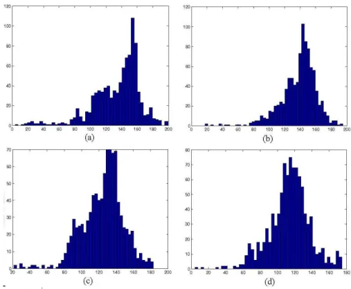
Figure 3.6: The histograms of the corresponding patches which are shown in Figure 3.5
To find the scale in which the desired texture signature lies, we chose to use the kurtosis value of histogram of each patch in the neighborhood scale-space. Kurtosis is defined as
Kurt(X) = µ4
σ4 − 3, (3.1)
which is the forth central moment normalized with respect to normal distri-bution. Sometimes it may be used without normalization as
µn = E((X − µ)n), (3.2)
in which n equals to 4.
Kurtosis measures the amount of deviation from the mean due to the peaks in the histogram. This measure implicitly shows how complicated the given