Range resolution improvement in passive coherent location radar systems using multiple FM radio channels

RANGE RESOLUTION IMPROVEMENT IN

PASSIVE COHERENT LOCATION RADAR

SYSTEMS USING MULTIPLE FM RADIO

CHANNELS

A THESIS

SUBMITTED TO THE DEPARTMENT OF ELECTRICAL AND ELECTRONICS ENGINEERING

AND THE INSTITUTE OF ENGINEERING AND SCIENCES OF BILKENT UNIVERSITY

IN PARTIAL FULLFILMENT OF THE REQUIREMENTS FOR THE DEGREE OF

MASTER OF SCIENCE

By

Akif Sinan TAŞDELEN

January 2007

ii

I certify that I have read this thesis and that in my opinion it is fully adequate, in scope and in quality, as a thesis for the degree of Master of Science.

Prof. Dr. Hayrettin Köymen (Supervisor)

I certify that I have read this thesis and that in my opinion it is fully adequate, in scope and in quality, as a thesis for the degree of Master of Science.

Prof. Dr. Ayhan Altıntaş

I certify that I have read this thesis and that in my opinion it is fully adequate, in scope and in quality, as a thesis for the degree of Master of Science.

Prof. Dr. İbrahim Körpeoğlu

Approved for the Institute of Engineering and Sciences:

Prof. Dr. Mehmet B. Baray

iii

ABSTRACT

RANGE RESOLUTION IMPROVEMENT IN PASSIVE

COHERENT LOCATION RADAR SYSTEMS USING

MULTIPLE FM RADIO CHANNELS

Akif Sinan Taşdelen

M.S. in Electrical and Electronics Engineering

Supervisor: Prof. Dr. Hayrettin Köymen

January 2007

Passive coherent location (PCL) radar systems that use single FM radio channel signal as illuminator of opportunity have reasonable Doppler resolution, but suffer from limited range resolution due to low modulation bandwidth and high dependence on the content that is being broadcasted from the FM station. An improvement in range resolution is obtained by using multiple adjacent FM channels, emitted from co-sited transmitters, which is often the case in large towns. The proposed scheme computes the autocorrelation function of the signal directly received from the co-located FM transmitter, and compares it to the cross-ambiguity function, obtained from direct and target scattered signals. The geometry of the problem is like in the case of monostatic radar. The range information is obtained by the delay between the cross-ambiguity function and the autocorrelation function. When a single FM channel that has a modulation bandwidth of 25 kHz is employed the range resolution is 6 km. It is shown that down to −33dB signal to noise ratio (SNR), which corresponds to a distance of 110 km from the receiver, targets that are 3 km separated from each other can be detected with 3 adjacent FM channels. It is possible to detect targets that are 100 m separated from each other with 7 FM channels. The detection of the time delays is a linear estimation problem.

Keywords: Passive coherent location (PCL), range resolution, modulation

iv

ÖZET

ÇOĞUL FM RADYO KANALI KULLANILARAK PASİF

TUTARLI KONUMLAMA RADAR SİSTEMLERİNDE

UZAKLIK ÇÖZÜNÜRLÜĞÜ ARTIRMA

Akif Sinan Taşdelen

Elektrik ve Elektronik Mühendisliği Bölümü Yüksek Lisans Tez Yöneticisi: Prof. Dr. Hayrettin Köymen

Ocak 2007

Kooperatif olmayan aydınlatıcı olarak tek FM radyo kanalı kullanan pasif tutarlı konumlama (PTK) radar sistemleri, makul Doppler çözünürlüğüne sahip olmalarına karşı, dar modülasyon bant genişliğinden, ve o an yayınlanın yayının içeriğine olan yüksek bağımlılıklarından dolayı sınırlı uzaklık çözünürlüğüne sahiptirler. FM radyo kanal dağılımının gevşek şekilde denetlendiği bazı ülkelerde bulanabileceği şekilde aynı vericilerden yayınlanan birden fazla FM radyo istasyonu kullanıldığı zaman uzaklık çözünürlüğünde bir gelişme elde edilebilir. Önerilen sistem, aynı yerde bulunan FM vericisinden alınan direk sinyalin öz ilinti fonksiyonunu hesaplar ve olası hedeflerden yansıyarak gelen sinyalin direk sinyalle olan çapraz ilinti fonksiyonuyla karşılaştırır. Problemin geometrisi monostatik radar sistemlerindeki gibidir. Uzaklık bilgisi çapraz ve öz ilinti fonksiyonlarının arasındaki zaman farkından elde edilir. Modülasyon bant genişliği 25 kHz olan tek bir FM istasyonu kullanıldığında 6 km uzaklık çözünürlüğü elde edilmektedir. Bu tezde gösterilmektedir ki, yanyana bulunan 3 FM radyo kanalının sinyallari kullanıldığında sinyal gürültü oranı (SGO) −33dB’ye inene kadar (ki bu 110 km uzaklığa tekamül etmektedir) aralarındaki uzaklık 3 km olan iki hedef başarıyla bulunabilir. 7 FM radyo kanalı ile birbirlerinden 100 m uzakta bulunan iki hedefi tespit etmek mümkündür.

Anahtar Kelimeler:.Pasif tutarlı konumlama, uzaklık çözünürlüğü, modülasyon

v

Acknowledgements

I would like to express my gratitude to Prof. Dr. Hayrettin Köymen for his supervision, encouragement and guidance throughout the development of this thesis.

I would also like to thank my family, Servet, Rânâ and Erdem Taşdelen, for their invaluable support, love and belief in me. I would express my special thanks to Gözde for her patience, confidence and unconditional love.

It is a pleasure for me to show deep appreciation for my friends in the ‘Synergy Room’, without whom the development of this thesis would have been much tiresome. I am also grateful to the guys of Chiba City for their morale support.

vi

Table of Contents

1. INTRODUCTION ... 1

1.1HISTORY OF PASSIVE COHERENT LOCATION... 2

1.2‘ILLUMINATORS OF OPPORTUNITY’ ... 4

1.3ORGANIZATION OF THE THESIS...6

2. RADAR AMBIGUITY FUNCTION ... 7

2.1THE MONOSTATIC RADAR AMBIGUITY FUNCTION...7

2.2THE BISTATIC RADAR AMBIGUITY FUNCTION... 10

2.3FMRADIO BROADCASTING...12

3. PCL USING MULTIPLE FM RADIO CHANNELS ... 16

3.1THE MOTIVATION...16

3.2PERFORMANCE PREDICTION... 18

3.3MINIMUM SNRCONDITION FOR DIRECT SIGNAL RECEPTION... 28

3.4DETECTION... 30

4. RANGE RESOLUTION IMPROVEMENT... 35

4.1RANGE RESOLUTION LIMITATIONS WHEN SINGLE FMCHANNEL IS EMPLOYED... 35

4.2RANGE RESOLUTION IMPROVEMENT WHEN 3FMCHANNELS ARE EMPLOYED... 41

4.3RANGE RESOLUTION IMPROVEMENT WHEN 7FMCHANNELS ARE EMPLOYED... 45

5. CONCLUSIONS...47

6. APPENDIX A...49

vii

List of Figures

Figure 2.1 North referenced coordinate system ... 11

Figure 2.2 Pre-emphasis filter fequency response... 13

Figure 2.3 Stereo FM radio spectrum... 13

Figure 2.4 One sided energy spectral density of kanun and ney duet ... 14

Figure 2.5 One sided energy spectral density of FM modulated signal, message signal being kanun and ney duet ... 14

Figure 2.6 One sided energy spectral density of Carmina Burana – O Fortuna. 15 Figure 2.7 One sided energy spectral density of FM modulated signal, message signal being Carmina Burana – O Fortuna... 15

Figure 3.1 Part of FM frequency spectrum recorded at Bilkent University, Ankara. Signals are transmitted from Çaldağı, Ankara... 17

Figure 3.2 Square wave ... 19

Figure 3.3 Spectrum of the square wave ... 20

Figure 3.4 Spectrum of the sum of a base-band square wave and a modulated square wave ... 20

Figure 3.5 Autocorrelation of the sum of a base-band square wave and a modulated square... 21

Figure 3.6 One-sided spectrum of the message signal ... 22

Figure 3.7 One-sided spectrum of the FM modulated signal ... 22

Figure 3.8 Ambiguity function of a single FM channel waveform... 23

Figure 3.9 One-sided spectra of the three message waveforms ... 24

Figure 3.10 One-sided spectrum of the signal containing 3 FM channels ... 24

Figure 3.11 Ambiguity function of three adjacent FM channel waveform... 25

Figure 3.12 Autocorrelation functions of single FM channel waveform and three adjacent FM channels waveform... 26

Figure 3.13 Autocorrelation function for seven adjacent FM stations... 27

viii

Figure 3.15 Autocorrelation function for single FM signal for various SNR .... 39 Figure 3.16 Autocorrelation function for seven adjacent FM signals for various

SNR ... 30 Figure 3.17 Block diagram of the detection algorithm ... 33 Figure 4.1 The autocorrelation of the directly received signal... 36 Figure 4.2 The cross-correlation of the direct signal and target scattered signal37 Figure 4.3(a) One-sided spectrum of the autocorrelation of the direct signal. (b)

One-sided spectrum of the cross-correlation of the direct and target scattered signals. (c) One-sided spectrum of the signal resulting from the division of auto- and cross-correlation spectrums after filtering operation 38 Figure 4.4 Real part of the IFFT of the division signal (1FM channel employed,

targets are 6 km separated, rectangular filter) ... 38 Figure 4.5 Tapered division signal ... 39 Figure 4.6 Real part of the IFFT of the division signal (1FM channel employed,

targets are 6 km separated, tapered division signal)... 39 Figure 4.7 Real part of the IFFT of the division signal (1FM channel employed,

targets are 3 km separated, rectangular filter) ... 40 Figure 4.8 Real part of the IFFT of the division signal (1FM channel employed,

targets are 3 km separated, tapered division signal)... 41 Figure 4.9 IFFT of the Division Signal after rectangular filtering... 42 Figure 4.10 Real part of the IFFT of the division signal (3FM channels

employed, targets are 6 km separated, rectangular filter) ... 42 Figure 4.11 Real part of the IFFT of the division signal (3FM channels

employed, targets are 6 km separated, tapered division signal ... 43 Figure 4.12 Real part of the IFFT of the division signal (3FM channels

employed, targets are 3 km separated, rectangular filter) ... 44 Figure 4.13 Real part of the IFFT of the division signal (3FM channels

employed, targets are 3 km separated, Gaussian filter)... 45 Figure 4.14 Real part of the IFFT of the division signal (7FM channels

1

Chapter 1

Introduction

On February 26, 1935 Robert Watson-Watt, an English scientist, conducted a simple experiment in a field near Daventry, UK, that proved that aircrafts can successfully detected by radio waves. The idea was that if an aircraft was 'illuminated' by radio waves, enough energy should be 'reflected' to permit detection on the ground by a sensitive receiver. The BBC had a powerful short-wave transmitter Station near Daventry, the Empire Radio Station, with a power output of 10 kW. The wavelength was 49m and the continuous beam was about 30 degrees wide and with a 10 degree elevation. An old Hadley Page Heyford bomber made a number of passes at differing altitudes from 6000 ft down to 1000 ft. The demonstration was a success: on several occasions a clear signal was seen from the bomber. This experiment, which is historically known as the Daventry Experiment, is, besides being the first radar experiment, a passive radar experiment [1, 2, 3, 4].

Passive radar systems, also known as passive coherent location (PCL) and passive covert radar, are radar systems that use non-cooperative illuminators, also referred as ‘illuminators of opportunity’, as sources of target illumination. Instead of transmitting optimally shaped waveforms with a dedicated

2

transmitter, which is the case in conventional radar systems, passive radar makes use of the telecommunication signals that are already in the air, such as analogue television or radio broadcast signals, GSM telephone signals etc (not to be confused with passive systems that perform imaging based on thermal body radiation).

The largest benefit of using non-cooperative illuminators is that it is almost impossible to detect, since the system has no transmitter of its own (this is where the name ‘passive’ comes from). It is a low cost system. Since the transmitter network is already built, the deployment and maintenance is easy. There is no frequency allocation needed.

The largest drawback of the system is that the waveform being transmitted and its power are not controllable. Therefore, the system has to operate with signals that may not be optimal for radar purposes. This means that high computational power is needed.

1.1 History of Passive Coherent Location

After the Daventry Experiment radar systems became a major field of research. Early radar systems were all bistatic, where the transmitter and receiver are not co-located. This was due to the fact that the technology to switch an antenna from transmitter to receiver mode was not developed yet. Examples like the British Chain Home system; the French “fence” system; the Soviet RUS-1; and the Japanese “Type-A” were all systems that had their own transmitters [5].

The Germans used a passive bistatic system, which they called the Kleine Heidelberg device, during World War II. The system was located at Ostend and was using the British Chain Home radar system as the non-cooperative illuminator to detect aircraft over the southern part of the North Sea [5].

3

Later, systems that designed and transmitted their own optimally shaped waveforms that could have high transmitted signal powers became dominant. These are now called conventional radars. Because of the high computational power requirement, passive coherent location radars became unattractive for researchers.

With the introduction of low cost computing power and digital receiver technology in the 1980’s the concept of passive radar systems became a popular research area, again. Now the designers could apply digital signal processing techniques to exploit variety of broadcast signals. The first commercial system that was announced by Lockheed-Martin Mission Systems in 1998 was the Silent Sentry that exploited FM radio and analogue television transmitters [6].

Besides Silent Sentry, currently there are working passive radar systems like BAe System’s CELLDAR that uses GSM basestations as illuminator of opportunity [7] and Thales Air Systems’ Homeland Alerter, an FM radio based passive radar.

The researches focus on two major topics: The problem of the geometry and the problem of the signal processing.

In [8] a methodology for finding possible receiver locations for passive radar is presented. It is stated that, because of the wide range of passive radar applications an optimal receiver location cannot be determined, but there are optimal solutions for each specific requirement. In [9] the constellation of multisensors in bearing-only location system is studied. In [10] a target location method based on time difference of arrival (TDOA) sequences with a two transmitter/one receiver (T2/R) passive radar is presented.

There are numerous techniques suggested for passive radar imaging. A Smoothed Pseudo Wigner-Ville Distribution (SPWVD)-based imaging

4

algorithm can be applied to reflected TV signals for target classification [11]. Some deconvolution techniques, such as the CLEAN algorithm, which is utilized for high-resolution target imaging at high-frequencies, can be applied to frequencies of interest in passive radar. This yields images that are more disturbed [12]. In [13] an optimization-based, region-enhanced image formation technique for the sparse aperture passive radar is explored. Compared to conventional direct Fourier transform-based imaging passive radar data, where artifacts are produced and characteristic features of the imaged objects are suppressed, the region-enhanced imaging approach is well suited for passive radar imaging. Roland Mahler’s probability hypothesis density (PHD) based multitarget tracking is investigated in [14]. To partially overcome the problem of high computational power requirement distributed passive radar processing through channelised data is suggested in [15].

1.2 ‘Illuminators of Opportunity’

Broadcast signals such as analogue television, FM radio and Digital Audio Broadcast (DAB) have high transmitter powers and excellent coverage. Due to these properties, they are attractive illuminators of opportunity for PCL applications.

At first glance, analogue television transmitters seem to be the obvious choice, because of their very high equivalent radiated powers and large bandwidth. However, the 64 µs line fly back time creates high side-lobes in the ambiguity function, resulting in range ambiguities at 19.2 km [16]. Using only a fraction of the analogue TV spectrum, which is very difficult due to the 15 kHz separation of the line fly backs, is not beneficial, since the power of each line fly back is very low compared to the total power. Howland showed that it is possible to extract Doppler and bearing information from echoes of analogue TV video carrier signal to track aircrafts at ranges up to 260 km from the receiver and 150 km from the transmitter [17]. Howland took the receiver bandwidth only a few

5

kilohertz, which is only a fraction of the total 5.5 MHz analogue TV spectrum. Therefore, this approach is named as ‘narrowband processing’. Due to the low information content in the Doppler measurements, the system must observe the target’s Doppler history for an extended period of time in order to locate the target at all. Furthermore, the location depends on the initial location estimate of the target.

In [18] the suitability of Global System of Mobile (GSM) communication signals for passive radar applications is investigated. It is shown by an implemented system that GSM based PCL can successfully detect and track ground-moving targets such as vehicles and humans. However, due to the low radiated power GSM signals are not well suited for air-borne target detection.

Digital broadcast signals such as Digital Television (DTV), Digital Audio Broadcast (DAB) and Digital Video Broadcast (DVB) are also sources of non-cooperative illumination. In [19] DAB is shown to have a coverage of around 9 km (where the SNR drops to 15dB). Poullin states in [20] that he has achieved a range resolution of 200 m with DAB. In [21] Saini and Cherniakov show that deterministic components in the DTV-T transmission introduce a number of undesired peaks in the ambiguity function that they try to eliminate with some algorithms. They conclude that DTV-T is a promising candidate for passive radar applications.

In [22] the global navigation satellite system (GNSS) is used as the non-cooperative illuminator. Two basic configurations are considered: the radar receiver is on an airplane; and positioned stationary on the ground. The system tries to detect objects on the ground. Another research on PCL using non-cooperative satellite (e.g. Globalstar or Global Positioning System (GPS)) as illuminator is [23] that focuses on the 2-D resolving capability within the ground plane.

6

In contrast to the narrowband processing, wideband processing utilizes almost all the spectrum of the waveform being exploited at the receiver. A typical single station FM broadcast waveform has 100 kHz bandwidth, which corresponds to a theoretical range resolution of 1500 m. Griffiths showed, however, that the effective bandwidth is not the whole 100 kHz, depending on the content being broadcasted, it can reach up to 24.4 kHz on the average for fast tempo jazz music, that shows the highest bandwidth [16]. Ambiguity plots that show on the average 30dB – 40dB peak to side-lobe ratios in range, and 30dB – 50dB peak to side-lobe ratios in Doppler demonstrate the performance of FM radio waveforms in PCL. These show that FM based PCL has a reasonable Doppler resolution, but a poor range resolution. In [24], Howland showed that an experimental radar system using a single station FM radio broadcast signal as illuminator of opportunity detects and tracks targets to ranges in excess of 150 km from the receiver. In [25] it is shown that FM based PLC can also be employed to observe auroral E-region irregularities.

1.3 Organization of the Thesis

This thesis is organized as follows: Chapter 2 explains the basics of radar ambiguity function for both monostatic and bistatic radar and the basics of FM radio broadcast. Chapter 3 introduces the idea of multiple FM radio channel PCL and investigates the performance in detail. In Chapter 4 simulations with 1 FM, 3 FM and 7 FM are done for closely separated targets. Finally, Chapter 5 concludes the thesis.

7

Chapter 2

The Radar Ambiguity Function

According to the geometry of the transmitter-receiver positioning, radar systems can be divided into three groups: Monostatic radar, bistatic radar and multistatic radar. Radar systems, where the transmitter and the receiver are co-located are called monostatic systems. Monostatic systems have the advantage of simple geometry. If the transmitter and receiver are located in different places, the system is called bistatic. Bistatic receivers systems have higher detection ability than monostatic radars when the head-on radar cross section of the target is small, and when the target scatters incident energy in different directions than the incident direction, which is the case in stealth fighters [26]. Multistatic radar systems are bistatic systems that use multiple receivers.

2.1 The Monostatic Radar Ambiguity Function

The radar ambiguity function is a well established measure in evaluating how well a waveform is suited for radar purposes [27]. It represents the output of a matched filter, where the signal is received with a time delay, τ, and a Doppler shift, υ, relative to the zeros expected by the filter [28]. In other words, the ambiguity function shows how similar a waveform is to its delayed versions in time and to its Doppler shifted versions in frequency. The radar ambiguity function is defined as:

( )

2 2 ) 2 exp( ) ( ) ( ,

∫

∞ ∞ − ∗ _{+ ⋅} ⋅ = Ατ υ s t s t τ j πυt dt (2.1)

The ambiguity function evaluated at (τ, υ) = (0, 0) is the output of a filter, which is perfectly matched to the received signal. It is shown in APPENDIX A that the value of the ambiguity function at this point is its global maximum.

8 2 2 ) 0 , 0 ( ) , ( A Aτ υ ≤ (2.2)

Thus, the three dimensional plot of the ambiguity function shows a peak at the origin.

Another useful property of the ambiguity function is that it is symmetric with respect to the origin.

2 2 ) , ( ) , (τ υ = A −τ −υ A (2.3)

This property shows that it is sufficient to study and plot only two adjacent quadrants of the ambiguity function.

The zero cuts of the ambiguity function, A(τ,0) andA(0,υ), give insight into

the range and Doppler properties of the waveform respectively.

∫

∞ ∞ − ∗ ₊ ⋅ = s t s t dt A(τ,0) ( ) ( τ) (2.4)

can be recognized as the autocorrelation function of the waveform. The autocorrelation function is a measure for the range resolution.

The minimum separation between two targets required for radar to distinguish between them is called the range resolution. Range resolution is a function of modulation bandwidth. The larger the modulation bandwidth of the waveform used in the radar the smaller is the range resolution. Since two closely spaced targets would reflect the incident waveform with a small delay in between, to distinguish those targets as two separate ones, the autocorrelation of the waveform has to have a sharp peak. In other words, the waveform and its delayed version should be ‘separated enough’ to distinguish the two reflections as two separate peaks in the ambiguity function. Equivalent to the range resolution, the delay resolution can be defined as the minimum time difference of two targets that can be successively resolved. Since waves travel at the speed of light, c, delay resolution can be obtained by dividing range resolution to c.

9

The motion of the target creates a Doppler shift in the frequency of the signal. The minimum Doppler shift required to distinguish between two targets is called the Doppler resolution. Doppler resolution is a function of the waveform and target illumination time. Alternatively, a velocity resolution can be defined as the minimum velocity difference between two targets to resolve them successfully. Velocity resolution can be obtained from the Doppler resolution by: λ υ ∆ = ∆v 2 (2.5) ∆v: velocity resolution ∆υ: Doppler resolution λ: wavelength

Like in the range ambiguity, a sharp peak in A(0,υ) is desired to better resolve two targets that have Doppler shifts close to each other (that are moving with a small speed difference).

Considering requirements both for range and Doppler, the best possible waveform would have an ambiguity function, which is a delta function at the origin, δ(0,0), with amplitude (2E)2, where E is the signal energy. The multiplicative constant is due to the constant volume property (see APPENDIX A). A signal with this property could locate the target at exact range and velocity. However, a signal having such an ambiguity function would require infinite bandwidth and infinite duration, which is practically impossible. Thus, regarding the application of the designed radar, ambiguity functions that approach δ(0,0) shape should be aimed.

Another way to define the monostatic ambiguity function is that it represents the Neyman-Pearson receiver. This receiver maximizes the detection probability for a specified false alarm probability, for detecting a slowly fluctuating point target at the hypothesized point (τH, ωH). The actual target location is (τa, ωa). In this

10

receiver, the ambiguity function is to be tested under two hypotheses, and compared to a threshold. The unknown nonrandom parameters τH, and ωH are to be estimated. The common expression for the ambiguity function is

(

, , ,

)

∫

~( ) ~ ( ) exp(

(

)

) 2 ∞ ∞ − ∗ _{− ⋅ − −} ⋅ − = s t s t j t dt Aτ_H τ_a ω_H ω_a τ_a τ_H ω_H ω_a (2.6)

Comparing equation (2.6) with equation (2.1) we note that τ =τ_a −τ_H and2πυ=ωa −ωH. Like mentioned above, τ is the time delay difference between the actual and hypothesized time delays. The autocorrelation reaches its maximum when τ = 0, meaning that the actual target delay is estimated. Likewise, υ is the difference between the actual Doppler shift and the hypothesized Doppler shift. The ambiguity function reaches its maximum when (τ, υ) = (0, 0).

2.2 The Bistatic Radar Ambiguity Function

In PCL applications receiver may, and in most cases will not be co-located with the illuminator. Therefore, the relative positions of transmitter, receiver and target plays a crucial role in ambiguity function calculation.

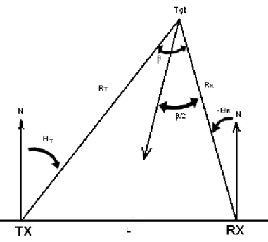
In [29] a geometry dependent definition of the Bistatic Ambiguity Function is introduced. This can be better be described by reffering to the north referenced coordinate system is given in Figure 2.1.

11

Figure 2.1. North-referenced coordinate system

The bistatic angle β is the angle at the apex of the bistatic triangle, and it is the sum of the transmitter’s look angle θT and the receiver’s look angle -θR. When the target is in the north of the baseline, β is in the interval [0,π]; when the target is to the south of the baseline, then β is in the interval [-π,0]. The line dividing the bistatic angle into two equal parts is called the bistatic bisector. RR and RT are the ranges from receiver to target and from transmitter to target, respectively. The sum of both ranges is called the total range, and is represented by R.

Any three of the four quantities θT, θR, L and R can completely specify a bistatic radar geometry. For instance

R R

R

T R L R L

R2 = 2 + 2 + 2 sin

θ

. (2.7)

Therefore the total transmission time delay is given by

(

R_R θ_R L

)

[

R_R R_R L R_RL θ_R

]

c

τ , , _{= +} 2 ₊ 2 ₊2 sin _{. (2.8)}

Likewise, the effective velocity is the sum of individual velocities. ⎟ ⎠ ⎞ ⎜ ⎝ ⎛ = + = 2 cos cos 2V φ β R dt d R dt d R dt d R T (2.9)

12 R R R R R L R L R L R θ θ β β sin 2 2 sin 2 1 2 cos 1 2 cos 2 2 _{+ +} + + = + = ⎟ ⎠ ⎞ ⎜ ⎝ ⎛ (2.10) is obtained. Thus the Doppler shift for a given target with velocity component along the bistatic bisector2Vcosφ, is given by

(

)

R R R R R c R R D L R L R L R V c f L V R f θ θ φ θ φ sin 2 2 sin 2 1 cos 2 , , cos , 2 2 _{+ +} + + = _(2.11)

Given equations (2.8) and (2.11) the bistatic ambiguity function can be expressed by

(

)

(

(

)

)

(

(

)

)

(

)

(

)

(

)

(

)

2 , , , , , , exp , , ~ , , ~ , , , , , dt t L V R L V R j L R t s L R t s L V V R R A R a R a R H R H R R H R R a R a H R R a H H a a H θ ω θ ω θ τ θ τ θ − − − ⋅ − = ∞

_∫

∞ − ∗ (2.12)

2.3 FM Radio Broadcasting

Invented in early 1930s, FM radio broadcasting became popular starting 1940s and is the most widely used modulation technique in radio broadcast. Although digital audio broadcast (DAB) starts to replace FM radio in several countries, it seems that it will still be used in developing countries for the near future. APPENDIX B contains the basics of frequency modulation.

FM radio broadcast utilizes the 87.5-108 MHz frequency band for voice and music transmission. The carrier frequencies of two adjacent channels are separated 100 kHz in some countries like UK, and 200 kHz in other countries like USA. However, radio stations that are broadcasted from co-sited transmitters are at least 300 kHz separated. In Turkey the separation is 200 kHz, but weakly controlled. The peak frequency deviation is fixed as ±75 kHz. In most countries the modulated signal is passed through a pre-emphasis filter, whose frequency response is given in Figure 2.2, to increase the performance of the demodulator in the presence of noise. The intermediate frequency, f_IF used

13

Figure 2.2. Pre-emphasis filter frequency response

The radio stations that transmit stereo radio music process the message signal before modulation. The sum and the difference of left and right microphone outputs are taken and a pilot tone is added for the separation process as seen in Figure 2.3. In stereo FM broadcast the bandwidth of the message signal is larger than in monophonic broadcast.

Figure 2.3. Stereo FM radio spectrum [30]

Below are two examples of monophonic wave files that are 0.1 seconds in length. First file is a kanun and ney (two traditional Turkish instruments) duet witch has a low bandwidth as seen in Figure 2.4. When this file is FM modulated, with carrier frequency 100 kHz, frequency deviation 50 kHz, the outcome is seen in Figure 2.5.

14 0 5000 10000 15000 0 10 20 30 40 50 60 70 frequency (Hz) am pl it u d e

Energy Spetral Density of file1

Figure 2.4. One sided energy spectral density of kanun and ney duet

0.4 0.6 0.8 1 1.2 1.4 1.6 x 105 0 200 400 600 800 1000 1200 1400 1600 1800 2000 frequency (Hz) am pl it u d e

Energy Pectral Density of FM modulated file1

Figure 2.5. One sided energy spectral density of FM modulated signal, message signal being kanun and ney duet

In Figure 2.6 the energy spectral density of another file with a full orchestra, playing Karl Orff’s Carmina Burana – O Fortuna, is depicted. The bandwidth is much wider. As seen from Figure 2.7, this waveform FM modulated has a wider modulation bandwidth than the first one.

15 0 5000 10000 15000 0 10 20 30 40 50 60 70 frequency (Hz) am pl it ude

Energy Spectral Density of file2

Figure 2.6. One sided energy spectral density of Carmina Burana – O Fortuna

0.4 0.6 0.8 1 1.2 1.4 1.6 x 105 0 200 400 600 800 1000 1200 1400 1600 1800 2000

Energy Spectral Density of FM modulated file2

frequency (Hz)

am

pl

it

ude

Figure 2.7. One sided energy spectral density of FM modulated signal, message signal being Carmina Burana – O Fortuna

16

Chapter 3

PCL Using Multiple FM Radio

Channels

3.1 The Motivation

The range resolution in constant false alarm rate (CFAR) radar systems is inversely proportional to the bandwidth of the waveform that is being used.

B c resolution Range 2 = (3.1)

In the above equation, c is the speed of light and B is the bandwidth of the signal. This relation suggests that range resolution in PCL systems that use FM radio broadcast as ‘illuminator of opportunity’ can be improved by increasing the total modulation bandwidth of the waveform. This can be done by making use of the signals of as many channels as required to achieve the aimed range resolution. The commercial FM radio broadcast spectrum 88-108 MHz suggests that hypothetically 20 MHz band can be exploited. Even if the modulation bandwidth corresponds to 10% of the total spectrum, 2 MHz, range resolution down to 75 m can be achieved.

In one service area, the carriers are separated at least by 300 kHz. In countries, where the FM radio channel allocations are weakly regulated, the maximum frequency deviations of the channels are faintly controlled. Frequencies that fall into the adjacent channel are not adequately suppressed, causing in metropolitan towns spectrum readings as seen in Figure 3.1. Interference between adjacent channels, are beneficial for the proposed system, although not desired in telecommunication. For instance, in Figure 3.1, the entire 94.7-95.6 MHz

17

spectrum or 96.5-97 MHz spectrum can be made use of, which has larger bandwidth than a single FM channel, yielding a better range resolution.

Figure 3.1. Part of FM frequency spectrum recorded at Bilkent University, Ankara. Signals are transmitted from Çaldağı, Ankara

In the above case, if the frequency band of 94.7-95.6 MHz is used we have a bandwidth of 900 kHz. As seen from equation 3.1, a bandwidth of 900 kHz results in a range resolution of 167 m. However, this is the case if the spectrum has equal power distribution. The power spectral density of the signal used is a slightly deviated version of triangular spectra. Thus the range resolution is expected to be somewhat larger than 167 m.

18

3.2 Performance Prediction

Due to Fourier transform property of the ambiguity function (see APPENDIX A)

( )

(

)

_∫

∞ ∞ − ∗ _{+ −} = − = A S f S f j f df Aτ,υ _XX υ, τ ( ) ( υ)exp( 2πτ) (3.2)

where S(f) is the Fourier transform of the signal s(t). Assuming the FM radio channels transmit the same content with same power, the spectrum of the signal being used is a sum of frequency shifted triangles, where each shift is equal to the carrier frequency of the individual channel. Thus, if n radio channels are used in the process the spectrum is represented by

∑

= − = n i c n f S f if S 0 ) ( ) ( (3.3)

where S(f) is the spectrum of an individual FM radio channel, and fc is the carrier spacing. Therefore the resulting ambiguity function is

(

)

∞

_∫

∞ − ∗ _{+ −} = − S f S f j f df AXX υ, τ n( ) n ( υ)exp( 2πτ) (3.4)

( )

_∫

∞ ∞ − ∗ ₊ = s t s t j t dt A τ,υ _n( ) _n ( τ)exp( 2πυ ) (3.5) where ) 2 exp( ) ( ) 2 exp( ) ( ) 2 exp( ) ( ) ( 0 0 t if j t s df ft j if f S df ft j f S t s c n i n i c n n π π π

∑

∫ ∑

∫

= ∞ ∞ − = ∞ ∞ − = ⎟ ⎠ ⎞ ⎜ ⎝ ⎛ − = = (3.6) Thus,

( )

dt t j t if j t s t if j t s A c n i c n i ) 2 exp( ) 2 exp( ) ( ) 2 exp( ) ( , 0 0 πυ π τ π υ τ ⎟ ⎠ ⎞ ⎜ ⎝ ⎛ _{+ −} ⎟ ⎠ ⎞ ⎜ ⎝ ⎛ =

∑

∫ ∑

= ∗ ∞ ∞ − = (3.7)

19

The shape of the ambiguity function for n FM radio channels is bounded by the ambiguity function of one FM channel. This result tells us that we can only improve by adding new radio channels.

Since the range resolution can be obtained from the autocorrelation function of the transmitted signal, it is beneficial to further investigate the properties of the autocorrelation function.

Assume we have a time limited signal s(t), as seen in Figure 3.2

⎪ ⎩ ⎪ ⎨ ⎧ < < < − − < = t T T t T T t t s p p p p 2 , 0 2 2 , 1 2 , 0 ) (

Figure 3.2. Square wave

20

Figure 3.3. Spectrum of the square wave

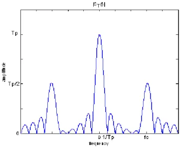
We note that the first zero occurs at 1/Tp. If a signal of the same spectral characteristics, but centered at fc = 6/Tp, is added to this signal, then we obtain the signal sT(t), with the spectrum given in Figure 3.4. This is equivalent to adding s(t)cos(2πfct) to s(t).

21

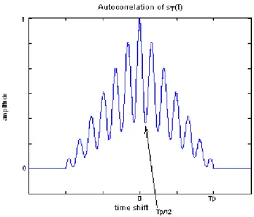
The resulting signal sT(t), has an autocorrelation function as depicted in Figure 3.5.

Figure 3.5. Autocorrelation of the sum of a base-band square wave and a modulated square wave

As seen from Figure 3.5, the first notch occurs at Tp/12 = 1/(2fc). Thus, we observe again, by increasing the total bandwidth the peak can be made narrower. Also we note that the envelope of the autocorrelation function of sT(t) is the autocorrelation function of s(t), i.e. a triangle.

In the following simulation the message signal is a 15 kHz filtered monophonic music file of 100 ms in length. The one-sided spectrum of the message signal is given in Figure 3.6.

22 0 5000 10000 15000 0 50 100 150 200 250 300 350

Spectrum of the message signal

frequency (Hz) am pl it u d e

Figure 3.6. One-sided spectrum of the message signal

The FM signal has a maximum frequency deviation of ± 75 kHz with no pre-emphasis. The one-sided spectrum of the frequency modulated signal is depicted in Figure 3.7. 0 0.2 0.4 0.6 0.8 1 1.2 1.4 1.6 1.8 2 x 105 0 2000 4000 6000 8000 10000 12000

Spectrum of the FM modulated signal

frequency (Hz)

am

pl

it

ude

23

The ambiguity function of a frequency modulated signal is given in Figure 3.8. Since the ambiguity function is symmetric for this signal, only a quarter is plotted.

Figure 3.8. Ambiguity function of a single FM channel waveform

In the following simulation three different waveforms of 100 ms length are employed as message signals. The one-sided spectra of the waveforms are depicted in Figure 3.9.

24 0 5000 10000 15000 0 100 200 300 400

Spectrum of the sound file1

frequency (Hz) am p lit ud e 0 5000 10000 15000 0 100 200 300

Spectrum of the sound file2

frequency (Hz) am pl it ud e 0 5000 10000 15000 0 200 400 600

Spectrum of the sound file3

frequency (Hz) am pl it ud e

Figure 3.9. One-sided spectra of the three message waveforms

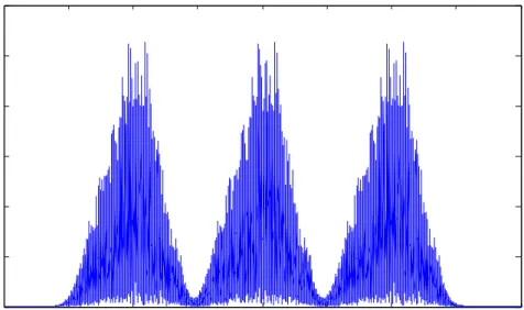
The one-sided spectrum of the signal containing 3 FM channels having 100 kHz equally spaced carrier frequencies is given in Figure 3.10.

0 0.5 1 1.5 2 2.5 3 3.5 4 x 105 0 2000 4000 6000 8000 10000 12000

Spectrum of the 3 equally spaced FM waveforms

frequency (Hz) am p lit ud e

25

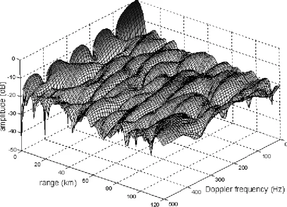
The ambiguity function of the signal containing three adjacent FM channels is depicted in Figure 3.11.

Figure 3.11. Ambiguity function of three adjacent FM channel waveform

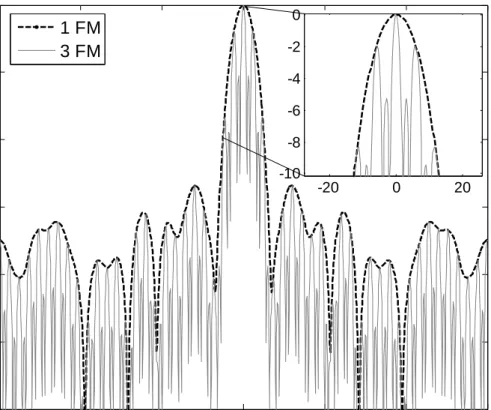
It is observed that the ambiguity function of the signal containing a single FM channel is an envelope to the ambiguity function of three FM station signal. The range resolution obtained by using only one FM channel, and the range resolution obtained from three adjacent stations that broadcast different content are depicted in Figure 3.12. Both signals have message contents with similar bandwidth.

26 -150 -100 -50 0 50 100 150 -30 -25 -20 -15 -10 -5 0

range (km)

ampl

it

ude (dB

)

-20 0 20 -10 -8 -6 -4 -2 0 1 FM 3 FM

Figure 3.12. Autocorrelation functions of single FM channel waveform and three adjacent FM channels waveform

The envelope of the autocorrelation function for three adjacent FM stations is the autocorrelation function for a single FM station. This is due to the fact that the spectrum of three adjacent FM station signals is almost like a 100 kHz repetition of a single FM station spectrum. Due to the periodic structure in the spectrum, a sinc type formation is observed in the range resolution plot. Since the modulation bandwidth is about three times the bandwidth of a single FM transmission, the peak in the autocorrelation function is narrower.

The peak can be made narrower when seven adjacent stations are used together (Figure 3.13.)

27 -150 -100 -50 0 50 100 150 -30 -25 -20 -15 -10 -5 0

range (km)

am

pl

it

ude (

d

B

)

-10 0 10 -10 -5 0

Figure 3.13. Autocorrelation function for seven adjacent FM stations

As in the three FM station case, the shape of the autocorrelation function of the waveform from seven adjacent FM stations resembles the autocorrelation plot of a single FM transmission. However some side-lobes are increased. Again, a sinc type formation is observed in the range resolution plot.

If stations are selected in a random way so that they are not adjacent, then the autocorrelation starts to lose its resemblance to the autocorrelation function of a single FM waveform. The autocorrelation function of seven FM signals having equal power, but distributed randomly in 1500 kHz bandwidth with minimum separation of 150 kHz and maximum separation 250 kHz is depicted in Figure 3.14.

28 -150 -100 -50 0 50 100 150 -30 -25 -20 -15 -10 -5 0

range (km)

am

pl

it

ude (

d

B

)

-10 0 10 -10 -5 0

Figure 3.14. Autocorrelation function for seven non-adjacent FM stations

As expected, the sinc type formation in the range resolution is lost due to the failed periodicity and the side-lobes in the vicinity of the peak are increased. However, the main peak is still narrow. Theoretically, the range resolution can be improved down to 2 km with an appropriate detection algorithm.

3.3 Minimum SNR Criterion for Direct Signal

Reception

In the analysis of the auto-ambiguity and autocorrelation functions the scattered signal is assumed to be noise free. As the received power of the scattered signal becomes smaller, the SNR decreases for far away targets. Consequently, the ambiguity function deteriorates, yielding a worse range resolution or even target loss or false alarm.

29

The proposed detection method depends on the minimum SNR that allows a successful detection of the autocorrelation function, buried in the cross-correlation. This is discussed in 3.4.

In the following simulations, the receiver noise is taken as white and Gaussian distributed, with spectral height of kT0B, where k is the Boltzmann constant, T0 is the temperature in Kelvin (taken as 300°K ) and B is the bandwidth. The bandwidth is 200 kHz in single FM signal simulation and 800 kHz in seven FM signals simulation, where the carriers are spaced at multiples of 100 kHz, and signal powers are equal. The signals are sampled at 5 MHz. Simulations show that for a single FM signal, the autocorrelation function preserves its shape down to −19dB SNR. For lower SNR the cross-correlation terms between signal and noise start to dominate. However, the peak of the autocorrelation is dominant down to −29dB as shown in Figure 3.15.

-60 -40 -20 0 20 40 60 -20 -18 -16 -14 -12 -10 -8 -6 -4 -2 0 range (km) am pl it ude ( d B ) -9.2 dB -19.2 dB -29.2 dB -39.2 dB

30

If the number of FM signals is increased, the autocorrelation shape shows no variation down to −6dB. The changes until −26dB are small and on the side-lobes. At −36dB the peak is no more dominant over the side-lobes (Figure 3.16).

-60 -40 -20 0 20 40 60 -20 -18 -16 -14 -12 -10 -8 -6 -4 -2 0 range (km) am pl it ude ( d B ) -6.8 dB -16.8 dB -36.8 dB

Figure 3.16. Autocorrelation function for seven adjacent FM signals for various SNR

This suggests that the direct signal receiver, if bistatic configuration is employed, should be at a distance to the FM transmitter, where SNR is at least −16 dB.

3.4 Detection

In [24] it is shown that the Doppler resolution of a PCL system, using FM radio broadcast as non-cooperative illuminator, is typically 1 Hz, corresponding to a velocity resolution of around 1.5 ms-1. The Doppler resolution can be improved by taking a longer integration time. In the analysis below it is assumed that the Doppler shift of the target is found by the radar and the signal is perfectly corrected in frequency.

31

Assume s(t) is broadcasted from a FM radio transmitter and received from a co-located receiver. This direct signal, s(t) at the receiver has a high SNR. The signal reflected from N targets and received from the receiver is represented by

) ( ) ( ) ( 1 t n t t s t s N i i i N =

∑

− + = α (3.8)

where αi is the attenuation constant for the signal scattered from the ith target, ti is the two-way time delay of the signal scattered from the ith target and n(t) is the zero mean white Gaussian noise process. The result of the cross-correlation of direct and target scattered signals is given by

) ( ) ( ) ( ) ( 1 τ τ τ α τ R t n s C N i i i − + • =

∑

= (3.9) where• denotes convolution and R is the autocorrelation of the direct signal and ns is the cross-correlation of the direct signal and noise. Taking the Fourier transform of the cross-correlation function, we obtain

{

( )

}

( ) ) 2 exp( ) ( ₀ 1 f S N R F ft j f C N i i i − + =

∑

= τ π α (3.10)

where F{R(τ)} is the Fourier transform of the autocorrelation function (the power spectral density), N0 = kT0B is the power spectral height of the white noise and S(f) is the Fourier transform of the direct signal. Dividing both sides by |S(f)|2 and applying the autocorrelation property of the Fourier transform we obtain 2 0 1 2 ) ( ) ( ) 2 exp( ) ( ) ( f S f S N ft j f S f C N i i i − + =

∑

= π α _(3.11) ) ( ) 2 exp( 0 1 S f N ft j N i i i ∗ = + − =

∑

α π (3.12)

where * denotes the complex conjugation. The problem reduces to finding the time shifts ti in the exponential. This is a linear estimation problem, and very good estimators are available. In the estimation problem for single channel FM signal, the estimation is done around one frequency, whose width determines the range resolution. The SNR around this frequency is higher than in other

32

frequencies. If, for instance, 3 FM channels are used, the estimation can be done around three frequencies, which implies that the range resolution is improved. The total signal power increases, but due to the additional bandwidth the noise power increases too. The total SNR, therefore, does not change. This results in the same detection performance as in the single FM channel case.

Taking the inverse Fourier transform of Equation 3.12 around the above mentioned frequencies is another way to find the time shifts ti. Due to the exponential term, the real part of the resulting function shows peaks at correct ti locations. In this approach however, time shifts can only be successfully extracted, where the additive term in Equation 3.12 is very small compared to the exponentials. The term in question is the inverse of the squareroot of SNR, and it is small at frequencies where the signal power is highest, namely at the vicinity of the carrier frequency. Thus, the frequencies where the SNR is low should be avoided in the computation. Effective filtering of the unwanted frequencies is another issue. While the easiest approach is to utilize bandpass filters with rectangular spectra, this can cause a sinc type shape in the inverse Fourier operation. Gaussian tapered or raised cosine shaped filters can be employed for better results. The detection algorithm is summerized in Figure 3.17.

33

Figure 3.17. Block diagram of the detection algorithm.

In the simulations of this thesis, the SNR is calculated as the total received signal power divided by the noise power after the filtering at the reception. The SNR at the detection stage is higher than the SNR at the reception, because the filter in the detection stage is carrier centered and has a bandwidth equal to the modulation bandwidth. This means that the total signal power remains almost the same, whereas the noise power is reduced. For example, when a single FM channel signal that is transmitted with 1kW power is reflected from two targets with RCS 10 m2 at 50 km and 56 km the SNR at the receiver with an

34

omnidirectioanl antenna is −15.1 dB, if the filter at the receiver has a bandwidth of 150 kHz. The SNR at the detection stage, where the detection filter bandwidth is taken to be 30 kHz, is calculated to be −9.9 dB.

35

Chapter 4

Range Resolution Improvement

4.1 Range Resolution Limitations When Single

FM Channel Is Employed

In the following simulations a 100ms monophonic sound file is low-pass filtered at 15 kHz and frequency modulated using MATLAB’s fmmod operation, the carrier frequency being 100 kHz and sampling frequency being 5 MHz. The resulting wave has maximum frequency deviation of ±75 kHz. No pre-emphasizing is employed.

The resulting signal is transmitted at 1 kW power with an omni-directional antenna having a gain of 1.64. The signal is assumed to be reflected from two targets, having radar cross sections of 10 m2, at distances of 50 km and 56 km from the transmitter. Since the modulation bandwidth of the FM signal is about 25 kHz, the range resolution is expected to be 6 km. The two targets should be successfully detected as being two separate targets. The received signals, which are delayed in accordance of the target distances, have powers calculated by the Radar Equation:

( )

3 4 2 4 r G G P Pr t t r π σ λ = (4.1) Pr: received power Pt: transmitted power Gt: transmitter antenna gain Gr: receiver antenna gain λ: wavelength

36 σ: radar cross section of the target

r: target’s distance to the receiver

The transmitter and receiver antennas are assumed to be co-sited. Assuming the radio station is transmitting at 100 MHz the wavelength is taken to be 3 m (since the commercial FM radio broadcast spectrum is 88-108 MHz the wavelength varies between 2.78 m and 3.41 m). The receiver antenna gain is taken to be 1, although directional antennas may be employed. Since only one FM station is used the bandwidth of the filter at the receiver is taken to be 150 kHz. Noise power, which is obtained by kT0B, is added to the signal. The SNR is calculated to be -15.1 dB.

The direct signal is taken to be the transmitter signal, because of the co-sited transmitter receiver pair. The detection is done as explained in 3.4.

The autocorrelation of the directly received signal is depicted in Figure 4.1

0 1 2 3 4 5 6 7 8 9 10 x 105 -1 -0.8 -0.6 -0.4 -0.2 0 0.2 0.4 0.6 0.8 1

Autocorrelation of the Direct Signal

time shift am pl it ud e 4.828 4.83 4.832 4.834 4.836 4.838 4.84 x 105 -1 -0.5 0 0.5 1

37

The cross-correlation of the direct signal and target scattered signal is shown in Figure 4.2. 0 2 4 6 8 10 12 x 105 -1 -0.8 -0.6 -0.4 -0.2 0 0.2 0.4 0.6 0.8 1

Crosscorrelation of the Direct and Target Scattered Signals

time shift am pl it ud e 5.028 5.03 5.032 5.034 5.036 5.038 5.04 5.042 5.044 x 105 -1 -0.5 0 0.5 1

Figure 4.2 The cross-correlation of the direct signal and target scattered signal

At this stage, we take the Fourier transforms of the auto- and cross-correlation functions. We divide the Fourier transform of the cross-correlation function to the Fourier transform of the autocorrelation function. The resulting signal is passed through a band-pass filter centered at the carrier frequency of the FM station, 100 kHz in our case.

The one-sided spectra of the autocorrelation and cross-correlation functions, as well as the resulting spectrum of the division operation, after the filtering operation, is shown on Figure 4.3.

38

Figure 4.3 (a) One-sided spectrum of the autocorrelation of the direct signal. (b) One-sided spectrum of the cross-correlation of the direct and target scattered signals. (c) One-sided spectrum of the signal resulting from the division of auto- and cross-correlation spectrums after

filtering operation.

By taking the inverse FFT (IFFT) of the division signal and plotting the real part of it Figure 4.4 is obtained. 10000 1200 1400 1600 1800 2000 2200 2400 2600 2800 3000 0.1 0.2 0.3 0.4 0.5 0.6 0.7 0.8 0.9 1

delay bin number

am

pl

it

ude

Real part of the IFFT of the Division Signal

Figure 4.4. Real part of the IFFT of the division signal (1FM channel employed, targets are 6 km separated, rectangular filter)

39

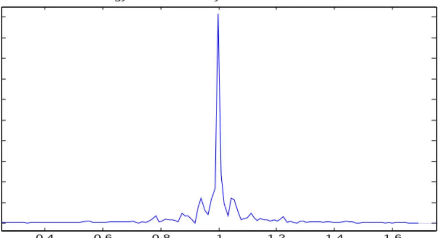
Figure 4.4 shows two peaks at delay bins 1667 and 1867. These two bins correspond to the distances 50.01 km and 56.01 km. Hence, the two targets are successfully detected at their true locations.

If the division signal is tapered (Figure 4.5), then the range resolution can be seen clearer (Figure 4.6). This comes to a cost of increased peak width. Two peaks are yet distinguishable.

0 0.2 0.4 0.6 0.8 1 1.2 1.4 1.6 1.8 2 x 105 0 0.1 0.2 0.3 0.4 0.5 0.6 0.7 0.8 0.9 1 frequency (Hz) am pl it ude

Tapered Division Signal

Figure 4.5 Tapered division signal

10000 1200 1400 1600 1800 2000 2200 2400 2600 2800 3000 0.1 0.2 0.3 0.4 0.5 0.6 0.7 0.8 0.9 1

delay bin number

am

pl

it

ude

Detection of 6 km separated targets with 1 FM (Gaussian filter)

Figure 4.6 Real part of the IFFT of the division signal (1FM channel employed, targets are 6 km separated, tapered division signal)

40

Simulations show that down to -30 dB SNR, which corresponds to a distance of 110 km from the receiver, the peaks due to the targets are 3 dB higher than the peaks due to noise. Thus a successful detection of two targets at 110 km distance to the receiver, having 6 km separation is possible with PCL employing single channel FM.

The following simulations are done with the same specifications. This time target1 and target2 are placed at 50 km and 53 km, respectively. Since the range resolution is around 6 km, we expect an error in the detection.

Figure 4.7 depicts the real part IFFT of the division signal where targets are 3km separated. 10000 1200 1400 1600 1800 2000 2200 2400 2600 2800 3000 0.1 0.2 0.3 0.4 0.5 0.6 0.7 0.8 0.9 1 frequency (Hz) am pl it ude

Detection of 3km separated taregets with 1FM channel

Figure 4.7 Real part of the IFFT of the division signal (1FM channel employed, targets are 3 km separated, rectangular filter)

From Figure 4.7 it can be seen that the two targets are no more detected as being two separate targets. Targets should be found in delay bins 1667 and 1700. Although the largest peak is found at 1667, there are further peaks at 1717, 1767, and 1618, which are false alarms. Furthermore, the second target is not detected at all. As expected, with one channel FM, targets that are closer to each other than the range resolution cannot be successfully distinguished as two separate targets.

41

If the division signal is tapered (Figure 4.8), it can be seen that the two peaks have merged to one single peak, which makes the detection of individual targets impossible. 10000 1200 1400 1600 1800 2000 2200 2400 2600 2800 3000 0.1 0.2 0.3 0.4 0.5 0.6 0.7 0.8 0.9 1

delay bin number

am

pl

it

ude

Detection of 3 km separated targets with 1 FM (Gaussian filter)

Figure 4.8 Real part of the IFFT of the division signal (1FM channel employed, targets are 3 km separated, tapered division signal)

4.2 Range Resolution Improvement When 3 FM

Channels Are Employed

In the following simulations three 100ms monophonic sound files with different contents are each low-pass filtered at 15 kHz and frequency modulated using MATLAB’s fmmod operation. The carrier frequencies are taken to be 100 kHz, 300 kHz and 400 kHz to simulate a weakly regulated environment. The sampling frequency is 5 MHz. The resulting waves have maximum frequency deviation of ±75 kHz. No pre-emphasizing is employed.

The resulting signal is transmitted at 1 kW power with an omni-directional antenna having a gain of 1.64. The signal is assumed to be reflected from two targets, having radar cross sections of 10 m2, at distances of 50 km and 56 km from the transmitter. Since three FM station are used, the bandwidth of the filter at the receiver is taken to be 500 kHz. Noise power, which is obtained by kT0B, is added to the signal. The SNR is calculated to be -20.4 dB. The reduction in

42

the SNR is due to the fact that the noise power increased with the wider filter bandwidth, whereas the signal power did not change.

At the detection step, after the division of the cross-correlation FFT to the autocorrelation FFT, the filter employed and the resulting spectrum are shown in Figure 4.9.

Figure 4.9 IFFT of the Division Signal after rectangular filtering

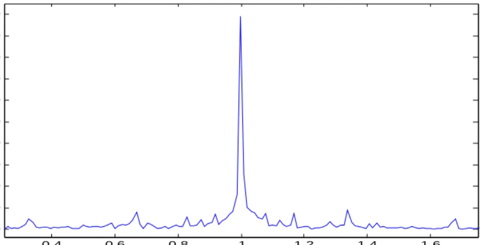
The IFFT of the division signal is depicted in Figure 4.10.

10000 1200 1400 1600 1800 2000 2200 2400 2600 2800 3000 0.1 0.2 0.3 0.4 0.5 0.6 0.7 0.8 0.9 1

Detection of 6 km separated targets wtih 3FM channels

delay bin number

am pl it u d e

Figure 4.10 Real part of the IFFT of the division signal (3FM channels employed, targets are 6 km separated, rectangular filter)

43

Two targets are successfully detected at delay bins 1667 and 1867, which correspond to the distances 50.01 km and 56.01 km, respectively.

If the division signal is tapered (Figure 4.11), range resolution can be seen better. 10000 1200 1400 1600 1800 2000 2200 2400 2600 2800 3000 0.1 0.2 0.3 0.4 0.5 0.6 0.7 0.8 0.9 1

delay bin number

am

pl

it

ude

Detection of 6 km separated targets with 3 FM (rectangular & Gaussian filter)

Figure 4.11 Real part of the IFFT of the division signal (3FM channels employed, targets are 6 km separated, tapered division signal)

This suggests that a more suitable filter can be found.

The following simulations are done with the same specifications. This time target1 and target2 are placed at 50 km and 53 km, respectively. Since the total bandwidth is increased, we expect an improvement in the range resolution so that the two targets are clearly distinguishable.

Figure 4.12 depicts the real part IFFT of the division signal, where targets are 3km separated, and 3FM channels are employed.

44 10000 1200 1400 1600 1800 2000 2200 2400 2600 2800 3000 0.1 0.2 0.3 0.4 0.5 0.6 0.7 0.8 0.9 1

delay bin number

am pl it u d e

Detection of 3 km spaced targets with 3 FM channels

Figure 4.12 Real part of the IFFT of the division signal (3FM channels employed, targets are 3 km separated, rectangular filter)

As seen from Figure 4.12 two targets at delay bins 1667 and 1767, which correspond to distances 50.01 km and 53.01 km, respectively, are successfully detected.

Simulations show that down to -33 dB SNR, which corresponds to a distance of 110 km from the receiver, the peaks due to the targets are 3 dB higher than the peaks due to noise. Thus a successful detection of two targets at 110 km distance to the receiver, having 3 km separation is possible with PCL employing 3 FM channels.

If instead of rectangular filter, a Gaussian filter is employed (Figure 4.13) the range resolution can be seen better.

45 10000 1200 1400 1600 1800 2000 2200 2400 2600 2800 3000 0.1 0.2 0.3 0.4 0.5 0.6 0.7 0.8 0.9 1

delay bin number

am

pl

it

ude

Detection of 3 km separated targets with 3 FM (Gaussian filter)

Figure 4.13 Real part of the IFFT of the division signal (3FM channels employed, targets are 3 km separated, Gaussian filter)

4.3 Range Resolution Improvement When 7 FM

Channels Are Employed

If it is possible to employ 7 FM channels, the range resolution can be made better, as depicted in Figure 4.14. Two targets are placed at 50 km and 50.1 km. Filter bandwidth is taken to be 1500 kHz. SNR is -24.4 dB.

10000 1200 1400 1600 1800 2000 2200 2400 2600 2800 3000 0.1 0.2 0.3 0.4 0.5 0.6 0.7 0.8 0.9 1

delay bin number

am

p

litu

d

e

Detection of 100 m spaced targets with 7 FM channels

1650 1655 1660 1665 1670 1675 1680 1685 1690 0.5 0.55 0.6 0.65 0.7 0.75 0.8 0.85 0.9 0.95 1

Figure 4.14 Real part of the IFFT of the division signal (7FM channels employed, targets are 100 m separated)

46

Two targets at delay bins 1667 and 1670, which correspond to distances 50.01 and 50.11 km, respectively, are successfully detected (Figure 4.14).

47

Chapter 5

Conclusions

Due to the increase in low cost digital signal processing power, Passive Coherent Location radar systems become more and more attractive for military as well as civilian applications. The passiveness of the system makes it an excellent choice for surveillance. Currently extensive research is done on improving PCL based systems.

FM radio broadcast signals are one of the appealing sets of non-cooperative illuminators for PCL. It has a reasonably good Doppler resolution, but a poor range resolution. Range resolution is inversely proportional to the transmitted signal bandwidth. The poor range resolution is due to the fact that only a fraction of the whole channel bandwidth, the modulation bandwidth, can be effectively used.

In this thesis, a system that employs multiple FM radio channels, instead of a single FM radio channel, is proposed and analyzed. A single FM radio channel based PCL, that can have 25 kHz modulation bandwidth, shows 6 km range resolution. It is shown that by employing 3 FM channels, two targets that are at ranges 50 km and 53 km from the receiver are successfully detected. When 7 FM channels are employed, two targets that are at ranges 50 km and 50.1 km from the receiver are successfully detected.

Simulations show that down to -33 dB SNR, which corresponds to a distance of 110 km from the receiver, the peaks due to the targets are 3 dB higher than the peaks due to noise. Thus a successful detection of two targets at 110 km distance to the receiver, having 3 km separation is possible.

48

In the detection, we employed rectangular and Gaussian tapered filters with fixed bandwidth. However, a dynamic filtering is likely to achieve better results, since the modulation bandwidth is a function of the content that is being broadcasted. A better filtering process should involve a measurement of the current modulation bandwidth on each channel and adjust the filter bandwidth accordingly.

The detection algorithm is based on a simple linear operation. A more sophisticated detection algorithm for time delay estimation can be utilized, such as nonnegative deconvolution [31]. A more complex detection and resolution refinement algorithm can be developed that first detects a target with a single FM channel utilizing CFAR detection, then utilizes multiple radio channels to refine the resolution of the area where the target was detected. This should decrease the computational complexity of the system.

In this thesis, only monostatic geometry is analyzed. It is expected that range resolution can be further improved when signals from multiple transmitters are employed with a single or multiple receiver configuration.

49

APPENDIX A

Here are two of the basic properties of Ambiguity function along with their proofs. Two other properties, which are not used in this thesis, are mentioned, but not proven here.

Property 1:

Maximum at (0,0) 2 2 2 ) 0 , 0 ( ) , ( A Es Aτ υ ≤ = (A.1)

WhereE is the energy of the signal. _s

Proof: We apply the Schwarz inequality to Equation A.1:

2 2 2 2 2 2 2 ) ( ) ( ) 2 exp( ) ( ) ( ) 2 exp( ) ( ) ( ) , ( s E dt t s dt t s dt t j t s dt t s dt t j t s t s A = + = + ≤ + =

∫

∫

∫

∫

∫

∞ ∞ − ∗ ∞ ∞ − ∞ ∞ − ∞ ∞ − ∗ ∞ ∞ − ∗ τ πυ τ πυ τ υ τ (A.2)

The imequality in Equation A.2 is replaced with an equality if the functions in the two integrals are the conjugates of each other, i.e:

[

( )exp( 2 )

]

( )exp( 2 ) )

(t s t j t s t j t

s = ∗ +τ πυ ∗ = +τ − πυ (A.3)

This only happens when τ = 0 and υ = 0. Hence, 2 2 2 ) 0 , 0 ( ) , ( A Es Aτ υ ≤ =

Property 2:

Symmetry with respect to the origin

2 2 ) , ( ) , ( τ υ Aτ υ A − − = (A.4)

50 2 2 ) 2 exp( ) ( ) ( ) , (

∫

∞ ∞ − ∗ _{− −} = − − s t s t j t dt A τ υ τ πυ (A.5)

and make a change of variable, t’= t - τ

(

)

(

)

(

)

2 2 2 2 2 2 ) , ( ) , ( 2 exp ) ( ) ( ' ' 2 exp ) ' ( ) ' ( ) 2 exp( ' ) ' ( 2 exp ) ' ( ) ' ( ) , ( υ τ υ τ πυ τ πυ τ πτ τ πυ τ υ τ A A dt t j t s t s dt t j t s t s j dt t j t s t s A = = − + = − + − = + − + = − − ∗ ∞ ∞ − ∗ ∞ ∞ − ∗ ∞ ∞ − ∗

∫

∫

∫

(A.6) Hence, 2 2 ) , ( ) , ( τ υ Aτ υ A − − =

Property 3:

Constant volume

2 2 . ) , ( d d Es A =

∫ ∫

∞ ∞ − ∞ ∞ − υ τ υ τ (A.7)

WhereE is the energy of the signal. s

Property 4:

Linear FM effect

If A(τ,υ)2 is the ambiguity function for the signal s(t)

2 ) , ( ) (t Aτ υ s ⇔

then adding linear frequency modulation (LFM) implies that

2 2_{) ( , )} exp( ) (t jπβt ⇔ Aτ υ −βτ s (A.8)