15
A BAYESIAN APPROACH FOR ITEM RESPONSE THEORY IN
ASSESSING THE PROGRESS TEST IN MEDICAL STUDENTS
Mehmet Ali Cengiz
1Zeynep Öztürk
21Ondokuz Mayıs University Department of Statistics, Turkey. 2Sinop University Department of Statistics, Turkey. E-Mail: [email protected] , [email protected]
Abstract
The progress test is used to provide useful summative and formative judgments about medical students' knowledge without distorting learning. The test samples the complete knowledge domain expected of new graduates on completion of their course, regardless of the year level of the student. Item Response Theory (IRT) have been proposed for evaluating examinations in medical education. Although IRT relies upon some strong assumptions, it is useful and practical in many situations such as medical education testing. IRT assumptions are often violated and threaten the statistical inferences. To overcome these difficulties, Bayesian approach to IRT can be used. The objective of this paper is to provide an overview of both Item Response Theory (IRT) and Bayesian IRT to the practitioner involved in the development of medical education assessments. We analysed the results from the Progress test examination taken by 4th year undergraduate medical students in the academic year 2010 to 2011. Advantages and disadvantages of IRT are initially described. Secondly, Bayesian approach for IRT is given. Bayesian approach is applied to IRT data set from Ondokuz Mayıs University. Finally, general recommendations to the use of Bayesian approach in practice are outlined. We found support for the use of Bayesian approach for IRT in assessing of progress testing.
Keywords: assessment Item Response Theory Progress test Bayesian approach medical students
Introduction
The progress test, invented concurrently by the University of Missouri-Kansas City School of Medicine and the University of Limburg, is used to provide useful summative and formative judgments about medical students' knowledge without distorting learning. All students in all classes sit the same examination at regular intervals through the year, and their individual progress is noted.
Progress tests are longitudinal, feedback oriented educational assessment tools for the evaluation of development and sustainability of cognitive knowledge during a learning process. A Progress Test is a written knowledge exam (usually involving multiple choice questions) that is usually administered to all students in a program at the same time and at regular intervals (usually twice to four times yearly) throughout the entire academic program. The test samples the complete knowledge domain expected of new graduates on completion of their course, regardless of the year level of the student. The differences between students’ knowledge levels show in the test scores; the further a student has progressed in the curriculum the higher the scores. As a result, these resultant scores provide a longitudinal repeated measure,
curriculum-independent assessment of the objectives (in knowledge) of the entire programme (Van der Vleuten et al. 1996).
Classical Test Theory (CTT) and Item Response Theory (IRT) have been proposed for evaluating examinations in medical education. IRT has many attractive features and advantages over CTT, which has contributed to its popularity in many measurement applications. Downing (2003) compares and contrasts IRT and CTT and explores of IRT in medical education. De Champlain (2010) provides an introduction to Classical Test Theory and IRT and how they can be applied to answer common assessment questions.
Although IRT relies upon some strong assumptions, it is useful and practical in many situations such as medical education testing. The IRT models describe a probabilistic relationship between the response an examinee provides on a test item, or items, and some latent trait, such as math or reading ability or some personality trait (De Boeck et al. 2004; Wainer et al. 2007). This article will define the popular unidimensional models and provide an interpretation for the parameters of these models.
16
IRT assumptions are often violated and threaten the statistical inferences. One of the challenges is to account for respondent heterogeneity and cross-classified hierarchical structures (Fox 2010). To overcome these difficulties, Bayesian approach to IRT can be used. Bayesian approach to IRT was firstly used by Tsutakawa (1984); Swaminathan et al.(1985) and Mislevy (1986). In Bayesian context, the response model parameters are described via prior models that present what we know about the parameter before observing the data.The objective of this paper is to provide an overview of Bayesian approach for IRT to the practitioner involved in the medical education assessments. The secondary aim of this paper is therefore to help the practitioner determine instances in which Bayesian approach might be preferable over classical IRT.
Material and Methods
The item response models developed in the 1970s and 1980s were mainly meant for analyzing item responses collected under standardized conditions in real test situations. İtem response theory rests on two basis. First is performance of a student on a test item can be predicted by a set of factors called traits, latent traits or abilities? Second is the relationship between students’ item performance and the set of traits underlying item performance can be defined by a monotonically increasing function called an item characteristic function and item characteristic curve.
The most general of the common dichotomous models is the three-parameter logistic model (3PLM), which is given below:
where is the probability of a correct response to item i , given an ability level of . The item parameters are , and and refer to characteristics of the items themselves.
The -parameter is often referred to as the item difficulty, and it is the point on the curve where the examinee has a probability of of answering the item correctly. In the case where is zero that corresponds to the point
where the examinee has a 50% chance of getting the item correct. The -parameter is on the same metric as the student ability parameter: . A student with an ability equivalent to the item difficulty will have a probability of of answering the
item correctly. A student with a higher ability will have a higher probability of a correct response, and a student with a lower ability will have a lower probability of a correct response. Though the scale for ability and difficulty parameters is arbitrary, most IRT software scales the student parameters so that 0 is the average, and that the standard deviation of the abilities is generally set to 1. This means that an item with a b-parameter of 0 is usually considered to be of average difficulty and that -value in general fall in the range of -3 to +3 (Hambleton, 1991).
The -parameter is commonly referred to as the item discrimination parameter, and is proportional to the slope of the tangent line at the point on the scale equal to the b-parameter. The higher the value, the more an item contributes to a student's ability estimate. Typically, it is desirable to have items with -values of 1 or higher, but content constraints and the difficulty of creating items with high discriminations at differing ability levels generally means that items with -values lower than 1 are often used.
The -parameter is the pseudo guessing parameter, or often, the guessing parameter, and is the height of the lower asymptote of the curve. This point provides the probability of a person of very low ability getting a correct response to the item.
Other popular IRT models are special cases of the more general three-parameter logistic model. The two-parameter model is the case where the c-parameter is set equal to zero. The one-parameter model, or the Rasch model, is obtained when the -parameters is zero and the a-parameter is set equal to 1 for all items. Use of these less general models is often called for in specific situations. In the context of an open response item, where the student does not have a high probability of guessing the right answer, a two-parameter model is a more appropriate choice. Under conditions where there are too few examinees to get high quality estimates of the - and -parameters, the one parameter model is often chosen. Though the one-parameter model provides less information about the item's true nature, the quality of the parameter estimate is often much higher under this condition and using less information of a higher quality is often preferable to using more information of lesser quality.
Bayesian Approach
In the Bayesian approach, model parameters are random variables and have prior distributions that reflect the uncertainty about the true values of the parameters before observing the data. The item response models discussed for the
17
observed data describe the data-generating process as a function of unknown parameters and are referred to as likelihood models. This is the part of the model that presents the density of the data conditional on the model parameters. Therefore, two modelling stages can be recognized: (1) the specification of a prior and (2) the specification of a likelihood model. After observing the data, the prior information is combined with the information from the data and a posterior distribution is constructed. Bayesian inferences are made conditional on the data, and inferences about parameters can be made directly from their posterior densities.Prior distributions of unknown model parameters are specified in such a way that they capture our beliefs about the situation before seeing the data. The Bayesian way of thinking is straightforward and simple. All kinds of information are assessed in probability distributions. Background information or context information is summarized in a prior distribution, and specific information via observed data is modelled in a conditional probability distribution. Objection to a Bayesian way of statistical inference is often based upon the selection of a prior distribution that is regarded as being arbitrary and subjective (see Gelman 2008). The specification of a prior is subjective since it presents the researcher's thought or ideas about the prior information that is available. In this context, the prior that captures the prior beliefs is the only correct prior. The prior choice can be disputable but is not arbitrary because it represents the researcher's thought. In this light, other non-Bayesian statistical methods are arbitrary since they are equally good and there is no formal principle for choosing between them. Prior information can also be based on observed data or relevant new information, or represent the opinion of an expert, which will result in less objection to the subjective prior. It is also possible to specify an objective prior that reflects complete ignorance about possible parameter values. Objective Bayesian methodology is based upon objective priors that can be used automatically and do not need subjective input. Incorporating prior information may improve the reliability of the statistical inferences. The responses are obtained in a real setting, and sources of information outside the data can be incorporated via a prior model. In such situations where there is little data-based information, prior information can improve the statistical inferences substantially. In high-dimensional problems, priors can impose an additional structure in the high-dimensional parameter spaces. Typically, hierarchical models are suitable for imposing priors that incorporate a structure related to a specific model requirement.
By imposing a structure via priors, the computational burden is often reduced.
Assume that response data are used to measure a latent variable that represents person characteristics. The expression represents the information that is available a priori without knowledge of the response data. This term is called the prior distribution or simply the prior. It will often indicate a population distribution of latent person characteristics that are under study. Then, it provides information about the population from which respondents for whom response data are available were randomly selected.
The term is the posterior density of the parameter given prior beliefs and sample information and is given as
where is likelihood function.
We use a two parameter IRT model for analyzing the progress test data. We define a standard normal prior for the ability parameters. Independence between the discrimination and difficulty parameters and a common normal distribution for both sets of parameters was assumed such that
, .
The hyperparameters and are normally distributed with means one and zero, respectively, and a large variance. The hyperparameters and have an inverse gamma prior with a small value for the shape and scale parameters.
MCMC Estimation
In the 1990s, several MCMC implementations were developed for logistic item response models. The developed simulation-based algorithms can be grouped using two MCMC sampling methods: Metropolis-Hastings (M-H) and Gibbs sampling. The Gibbs sampling method was used by Albert (1992) for the two-parameter normal ogive model (see also Albert 1993) The Gibbs sampling implementation of Albert (1992) is characterized by the fact that all full conditionals can be obtained in closed form and it is possible to directly sample from them given augmented data. This approach has been extended in several directions, and several expansions will be considered in subsequent chapters. Combining Gibbs sampling with M-H sampling leads to an M-H within Gibbs algorithm that turns out to be a powerful technique for obtaining samples from the target distribution (see Chib 1995, for a general description). Patz et al.(1999a) and (1999b) proposed an M-H within Gibbs sampler for several logistic response models.
18
Their M-H within Gibbs scheme is extended by allowing within-item dependencies and treating the hyper parameters as unknown model parameters. In each M-H step, the so-called candidate-generating density equals a normal proposal density with its mean at the current state. Then, the acceptance ratio is defined by a posterior probability ratio since the proposal density is symmetric.Results
We analyse the results from the Progress test examination taken by 4th year undergraduate medical students in the academic year 2010 to 2011
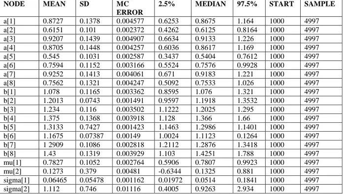
We take into account given answers to 8 question a randomly chosen from 71 question and, difficulties and discriminations of this questions are examined. We use the two parameter logistic model since the items are short-answer scored correct or incorrect. Using Winbugs problem Spiegelhalter (2004), The MCMC algorithm was run for 4997 iterations with first 1000 iteration as a burn-in. Table 1 contains posterior summaries of item parameters and the hyperparameters for a set of 8 multiple choice and open ended items that are scored as either correct(1) or incorrect(0)
Table 1 Posterior summaries for the two parameter logistic model.
NODE MEAN SD MC
ERROR
2.5% MEDIAN 97.5% START SAMPLE a[1] 0.8727 0.1378 0.004577 0.6253 0.8675 1.164 1000 4997 a[2] 0.6151 0.101 0.002372 0.4262 0.6125 0.8164 1000 4997 a[3] 0.9207 0.1439 0.004907 0.6634 0.9133 1.226 1000 4997 a[4] 0.8705 0.1448 0.004257 0.6036 0.8617 1.169 1000 4997 a[5] 0.545 0.1031 0.002587 0.3437 0.5404 0.7612 1000 4997 a[6] 0.7594 0.1152 0.003166 0.5524 0.7576 0.9928 1000 4997 a[7] 0.9252 0.1413 0.004061 0.671 0.9183 1.221 1000 4997 a[8] 0.7562 0.1321 0.004247 0.5092 0.7533 1.026 1000 4997 b[1] 1.078 0.1165 0.003362 0.8595 1.076 1.321 1000 4997 b[2] 1.2013 0.0743 0.001491 0.9597 1.1918 1.3532 1000 4997 b[3] 1.234 0.116 0.003502 1.1222 1.2025 1.295 1000 4997 b[4] 1.375 0.1368 0.003918 1.128 1.366 1.66 1000 4997 b[5] 1.3133 0.7427 0.001423 1.1463 1.2986 1.1401 1000 4997 b[6] 1.1675 0.07387 0.00149 1.0024 1.1123 0.1264 1000 4997 b[7] 1 2909 0.1086 0.002818 1.2112 1.2876 1.3418 1000 4997 b[8] 1.43 0.1319 0.003929 1.103 1.4251 1.788 1000 4997 mu[1] 0.7827 0.1052 0.002764 0.5906 0.7807 0.9923 1000 4997 mu[2] 0.1273 0.379 0.00481 -0.6344 0.1325 0.881 1000 4997 sigma[1] 0.06465 0.05478 0.001162 0.01972 0.0514 0.1841 1000 4997 sigma[2] 1.112 0.746 0.01116 0.4005 0.9263 2.934 1000 4997 For convergence diagnostics test, we use the rule of
thumb that says that MC error should be less than 5% of posterior SD. From Table 1, it can be seen that convergence was reached for all parameters. From Table 1, It can be seen that the items discriminate quite well and there is not much variation in discrimination values and it is easy to say that the test is fairly difficult since all of the -parameters are positive. Item eight, four, five and
seven appear to be much more difficult than the other items.
To compare classic item response models and Bayesian item response model fitted to our progress test data, the Akaike Information Criterion (AIC) and the Bayesian Information Criterion (BIC) can be used as a summary measure of fit. Given any two estimated models, the model with the lower value of AIC and BIC is the one to be preferred. We calculated the AIC and the BIC values for both classical and Bayesian approach for IRT as Table 2.
Table2. AIC and BIC values for Classic and Bayesian IRT
CRITERIA
APPROACHES
Classical IRT Bayesian IRT
AIC 314.451 246.853
19 AIC and BIC values for Bayesian IRT are much smaller than the AIC and the BIC values for classical IRT. So we prefer Bayesian IRT to classical IRT.
Discussion
IRT models have been used extensively over the past decades in medical education assessment programmes. Classical IRT makes much stronger assumptions and minimal sample size requirements for some of the simpler IRT models may not be feasible for some classes. Therefore Bayesian approach for IRT offers much flexible ideas. Bayesian approach can be use easily in the item response analysis. As models become more complex, more care needs to be taken over prior choice and convergence. When using Gibbs sampling for parameter estimation in the WinBUGS, which is very flexible, and can be used in a wide range of models to sample from the posterior distribution, the number of iterations to avoid convergence problem should be taken into account. Thumb rule can be followed.
References
1. Albert, J.H. (1992). Bayesian estimation of normal ogive item response curves using Gibbs sampling. Journal of Educational Statistics,; 17: 251-69.
2. Albert J.H., & Chib S. (1993). Bayesian analysis for binary and polychotomous response data. Journal of the American
Statistical Association; 88: 669-79.
3. Chib S., & Greenberg E. (1995). Understanding the Metropolis-Hastings algorithm. The American Statistician 49: 327-335.
4. De Boeck, P., & Wilson M. (2004).
Explanatory Item Response Models: A Generalized Linear and Nonlinear Approach.
New York Springer.
5. De Champlain, A.F. (2010). A primer on classical test theory and item response theory for assessments in medical education. Medical
Education; 44:109-17.
6. Downing, S. M. (2003). Item response theory: Applications of modern test theory in medical education. Medical Education; 37:739–45. 7. Fox, J.P. ( 2010). Bayesian Item Response
Modelling Theory and Applications. New York
Springer.
8. Gelman, A. (2008). Objections to Bayesian statistics. Bayesian Analysis; 3: 445-50. 9. Hambleton, R. K, Swaminathan, H.,& Rogers
J. (1991). Fundamentals of Item Response
Theory. Newbury Park, CA: Sage Publications
10. Mislevy, RJ. Bayes model estimation in item response models. Psychometrika, 1986; 51:177-95.
11. Patz ,R.J., & Junker, B. W. (1999a). Applications and extensions of MCMC in IRT:
Multiple item types, missing data, and rated responses. Journal of Educational and Behavioral Statistics; 24: 342-66.
12. Patz ,R.J., & Junker, B.W. (1999b). A straightforward approach to Markov chain Monte Carlo methods for item response models. Journal of Educational and Behavioral
Statistics; 24: 146-78.
13. Spiegelhalter, D., Thomas, A., Best, N., & Lunn, D. (2004). WinBUGS Version1.4 User Manual. MRC Biostatistics Unit. URL http://www.mrc-bsu.cam.ac.uk/bugs/.
14. Swaminathan, H., & Gifford, J.A.(1985). Bayesian estimation in the two parameter logistic model. Psychometrika; 50: 349-64. 15. Tsutakawa, R.K. (1984). Estimation of
two-parameter logistic item response curves.
Journal of Educational Statistics; 9: 263-76.
16. Van der Vleuten, C.P.M, Verwijnen, G.M.,& Wijnen, W.H.F.W.(1996). Fifteen years of experience with progress testing in a problem-based learning curriculum. Medical Teacher; 18:103–10.
17. Wainer H., Bradlow E.T, Wang X.(2007).
Testlet Response Theory and its Applications.