Locality-aware and load-balanced static task scheduling for MapReduce

(1)

Contents lists available atScienceDirect

Future Generation Computer Systems

journal homepage:www.elsevier.com/locate/fgcs

Locality-aware and load-balanced static task scheduling for

MapReduce

✩

Oguz Selvitopi

a

,

Gunduz Vehbi Demirci

a

,

Ata Turk

b

,

Cevdet Aykanat

a,

*

a_{Bilkent University, Computer Engineering Department, 06800, Ankara, Turkey} b_{Boston University, ECE Department, Boston, MA 02215, United States}

h i g h l i g h t s

• We propose models to simultaneously schedule map and reduce tasks in a MapReduce job.

• Our models exploit the pattern of the relations between mappers and reducers.

• A two-constraint formulation balances processors’ loads in both map and reduce phases.

• Our models improve the parallel runtimes of two key operations within the MapReduce.

a r t i c l e i n f o

Article history:

Received 24 December 2017 Received in revised form 5 May 2018 Accepted 20 June 2018

Available online 27 July 2018

Keywords: MapReduce Scheduling Data locality Load balance Map task Reduce task a b s t r a c t

Task scheduling for MapReduce jobs has been an active area of research with the objective of decreasing the amount of data transferred during the shuffle phase via exploiting data locality. In the literature, generally only the scheduling of reduce tasks is considered with the assumption that scheduling of map tasks is already determined by the input data placement. However, in cloud or HPC deployments of MapReduce, the input data is located in a remote storage and scheduling map tasks gains importance. Here, we propose models for simultaneous scheduling of map and reduce tasks in order to improve data locality and balance the processors’ loads in both map and reduce phases. Our approach is based on graph and hypergraph models which correctly encode the interactions between map and reduce tasks. Partitions produced by these models are decoded to schedule map and reduce tasks. A two-constraint formulation utilized in these models enables balancing processors’ loads in both map and reduce phases. The partitioning objective in the hypergraph models correctly encapsulates the minimization of data transfer when a local combine step is performed prior to shuffle, whereas the partitioning objective in the graph models achieve the same feat when a local combine is not performed. We show the validity of our scheduling on the MapReduce parallelizations of two important kernel operations – sparse matrix– vector multiplication (SpMV) and generalized sparse matrix–matrix multiplication (SpGEMM) – that are widely encountered in big data analytics and scientific computations. Compared to random scheduling, our models lead to tremendous savings in data transfer by reducing data traffic from several hundreds of megabytes to just a few megabytes in the shuffle phase and consequently leading up to 2.6x and 4.2x speedup for SpMV and SpGEMM, respectively.

✩_{This work was supported by The Scientific and Technological Research Council}

of Turkey (TUBITAK) under Grant EEEAG-115E212 and ICT COST Action, Turkey IC1406 (cHiPSet).

*

Corresponding author.

E-mail addresses:reha@cs.bilkent.edu.tr(O. Selvitopi),

gunduz.demirci@cs.bilkent.edu.tr(G.V. Demirci),ataturk@bu.edu(A. Turk), aykanat@cs.bilkent.edu.tr(C. Aykanat).

1. Introduction

MapReduce [1] simplifies the programming for large-scale data-parallel applications and greatly reduces the development effort by sparing the programmer from complex issues such as par-allel execution, fault tolerance, data management, task scheduling, etc. Hadoop [2], an open source implementation of MapReduce, has been used in production environments of many big companies and is deployed on clusters that can scale up to tens of thousands

(2)

of cores. Its generality, ease of use and scalability led to a wide acceptance and adoption in many fields.

A MapReduce job consists of map, shuffle and reduce phases which are carried out one after another by multiple parallel tasks that process data in parallel. The map tasks process the input data and emit

⟨

key

, v

alue

⟩

(KV) pairs. In the shuffle phase, the KV pairs are communicated and then they are sorted according to keys, thus grouping the values that belong to the same key. The reduce tasks then process the grouped values for keys and produce the final outputs belonging to keys. The tasks in a phase depend on the tasks in the preceding phase.

The performance of MapReduce jobs has been focus of interest in the literature. The studies that aim at improving the parallel performance of a MapReduce job generally either try to reduce data transfers during the shuffle phase [3–8] or try to balance the loads in the map and/or reduce phases [5,9]. Task scheduling studies usually focus on only the assignment of reduce tasks with the belief that map scheduling is determined by the initial data distribution of the file system hosted on the MapReduce compute nodes. However, in cloud or high performance computing deploy-ments of MapReduce this assumption is not valid. The input data often resides in a remote shared file system such as Lustre [10], or distributed object store such as Amazon S3 [11]. In such a setup, since all the data is loaded from a remote location, the scheduling of map tasks also becomes important.

In recent years, the MapReduce framework has attracted in-terest from the graph processing, machine learning, and scientific computing domains and there have been many studies towards parallelizing kernel operations in these fields using MapReduce. Examples include HAMA [12], Apache Mahout [13], MR-MPI [14] and [15]. In these domains, since the interactions among map and reduce tasks can be predetermined by a scan of the input datasets, and the applications often perform multiple iterations of MapRe-duce computations, intelligently scheduling map and reMapRe-duce tasks can yield significant performance gains.

In this work we propose a task assignment mechanism that simultaneously schedules map and reduce tasks to improve the performance of applications. Our contributions in this work can summarized as follows:

•

We propose models based on graph and hypergraph par-titioning to achieve a static scheduling of map and reduce tasks in a MapReduce job. The aims of our models are to attain locality among map and reduce tasks, and to balance computations at each processor. The locality in task assign-ment reduces the amount of data transfer in the shuffle phase and balancing of computations leads to faster task execution.

•

We show how our models can be utilized in a MapReduce framework. Our models’ outputs are used as hash functions to distribute KV pairs to mappers and reducers, i.e., we make use of application-specific knowledge to schedule map and reduce tasks.

•

We showcase the impact of our approach by improving the performance of two kernel operations: sparse matrix– vector multiplication (SpMV) and generalized sparse matrix-matrix multiplication (SpGEMM). We present algo-rithms for implementing these two operations in a MapRe-duce framework and describe how to use our models within them. In that sense, our models can be seen as improve-ments to the existing algorithms.

•

The models’ success of exploiting domain-specific knowl-edge in assigning tasks are validated with comprehensive experiments. Compared to random scheduling, the models lead to tremendous savings in data transfer in the shuffle phase, which leads up to 2.6x and 4.2x speedup for SpMV and SpGEMM, respectively.

SpMV is a common primitive that is encountered widely in numerical algebra [16] and iterative computations such as PageR-ank [17]. SpGEMM occurs in multigrid interpolation and restric-tion [18], linear programming [19], multi-source breadth first search [20], similarity join [21] and item-to-item collaborative filtering in recommendation systems [22]. The omnipresence of these kernel operations in machine learning, graph algorithms, and scientific computations make them attractive targets for perfor-mance optimization.

The rest of the paper is organized as follows. The related work and background are given in Section2. MapReduce parallelizations of SpMV and SpGEMM operations are respectively investigated in Sections5and6. Section7 presents the experiments. Section8

concludes.

2. Related work

Scheduling jobs and tasks for MapReduce programs has been an active area of research since the popularization of MapReduce paradigm. Job scheduling [23–28] considers allocation and usage of the resources in case of multiple MapReduce jobs. Task scheduling, on the other hand, focuses on the assignment of map and reduce tasks regarding a single MapReduce job. Our work falls in the latter category, so we focus on the works in this category.

Task scheduling presents two challenges which are critical for parallel performance: balancing the load in map and reduce phases, and decreasing the communication in the shuffle phase. Both can be alleviated via various approaches depending on the environment and the application MapReduce is being realized. The approach proposed by [3] considers data locality for decreasing communication in the shuffle phase and schedules each reduce task to its center-of-gravity node. This node is determined by two main factors: network locations of this reduce task’s feeders and the partitioning skew regarding this task. Similarly, the authors in [4] argue the overhead of the large network traffic and exploit data locality on both map and reduce phases to decrease the network traffic. Data locality is achieved by considering factors related to virtual machine placement, properties of the MapReduce job being run and the system load. [5] proposes a locality-aware approach based on a cost model that schedules reduce tasks in order to decrease the amount of data transferred in the shuffle phase. This approach is similar to our work in the sense that it also makes use of hash functions in order to decrease the data transferred in the shuffle phase and balance the load in reduce phase. Our work uses the hash functions in a static manner where they are determined from the patterns inherent in the input data, while in [5] they are determined on-the-fly according to the key frequencies. Another locality-aware approach is studied by [6], in which a scheduler called LARTS makes use of the information about the network locations and partition sizes in the scheduling decisions. LARTS improves data locality by reduce task scheduling and hence is able to decrease the network traffic. In [7], the authors propose a method that monitors the execution of MapReduce jobs and schedules map and reduce tasks according to the pattern deduced. By doing so they are able to schedule tasks preserving locality hence able to decrease the amount of transferred data in the shuffle phase. Recently, the authors of [8] propose an algorithm to improve the data locality and further overlap local reduce and shuffle phases of MapReduce jobs. Another study [9] aims to bal-ance the load in the reduce phase by collecting the key distribution of intermediate pairs and running an algorithm that utilizes this data to further make the scheduling decisions. The works in [29–

31] all aim at decreasing communication overheads: [29] by over-lapping map and shuffle phases, [30] by overlapping shuffle and reduce phases, and [31] with a barrier-less MapReduce framework. These studies do not consider data locality.

(3)

Most of these works perform dynamic scheduling and do not focus on improving the performance of a specific operation. Our approach is static, i.e., in a preprocessing stage we determine hash functions to exploit the target operation realized within the MapReduce paradigm. Most of the dynamic scheduling techniques for the tasks in a MapReduce job rely on scheduling only the reduce tasks in order to reduce data transfer in the shuffle phase and less often in order to balance the loads of the processors in the reduce phase. They usually do not handle scheduling of map tasks, i.e., clustering of map tasks on to same machines that produce values for the same keys. They rightly do so since this information largely depends on the application and it is usually not possible to know it in advance without perhaps running the application beforehand to collect information, or using application-specific knowledge to infer relations among tasks — which is the case in our approach. This also constitutes the main difference between static and dynamic scheduling methods.

Although dynamic scheduling approaches are more general than ours and may lead to runtime improvements in a MapReduce job, it can be said that only scheduling reduce tasks and without proper scheduling of map tasks, the improvements in data transfer in the shuffle phase would be minuscule compared to the gains obtained with a static approach at the expense of a preprocessing stage (our methods are able to reduce the amount of data transfers from several hundreds of megabytes to a few megabytes). More-over, as dynamic scheduling techniques do not aim at balancing the loads in the map phase and since the map phase is much more ex-pensive than the reduce phase for the operations evaluated in this work, a dynamic scheduling approach is highly unlikely to yield a better computation time than the proposed static scheduling.

3. Background

We realized the subject operations using MR-MPI library [14]. This library uses MPI for handling communication between proces-sors and in that sense it is fast and flexible. However, these come at the expense of fault tolerance and redundancy, both of which may prove vital in a commodity cluster but are not of prime concern on high performance computing systems. The high performance com-puting systems, sometimes called tier-0 systems, are characterized with very high availability and they allow access to full resources, without any virtualization or whatsoever. As our focus in this work is such a system, we preferred MR-MPI for implementation.

MR-MPI library supports two basic data types on which the functions operate:

⟨

Key

,

Value

⟩

(KV) and

⟨

Key

,

Multi

v

alue

⟩

(KMV). As the name suggests, a KMV pair stores all values related to a key while a KV pair stores a single one of them. The operations that are of interest to our work in this library are briefly described below:

•

map(): Generates KV pairs.

•

reduce(): Reduces KMV pairs to KV pairs.

•

collate(): Communicates KV pairs and generates KMV pairs

from them. Equivalent to MapReduce shuffle.

•

aggregate(): Distributes KV pairs among processors.

Neces-sitates communication.

•

con

v

ert(): Creates KMV pairs from KV pairs in which the

values belonging to the same key become a MultiValue.

•

add(): Adds KV pairs of a MapReduce object to those of

another.

These operations are used in our implementation. For more details on MR-MPI, see [14].

4. Modeling MapReduce applications

The map and reduce tasks in a MapReduce job can be sched-uled with certain considerations in mind if the relations between map and reduce tasks are known apriori. These relations may be inferred from the target application’s computational structure on the input data or the MapReduce job can be run beforehand to infer them. The latter case is particularly useful if the same MapReduce job will be executed multiple times. In this section, we show how the map and reduce tasks can be scheduled via graph and hypergraph partitioning models to address important issues such as load balancing and communication reduction.

Consider a setMof map tasks and a setRof reduce tasks, where the time to execute a map task mi

∈

Mand a reduce

task rj

∈

R is respectively denoted with size(mi) and size(rj).

A KV pair is denoted with the tuple

⟨

key

, v

al

⟩

. The set of KV pairs generated by mi is denoted by k

v

p(mi) and the set of KV

pairs destined for rj is denoted by k

v

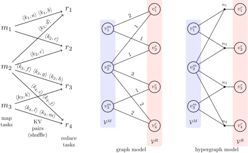
p(rj). Note that it is

as-sumed that the relation between map and reduce tasks is known, i.e., it is known that which map task produces value(s) for a certain key. The left ofFig. 1shows an example MapReduce job with three map and four reduce tasks. For example, k

v

p(m2)

=

{⟨

k1

,

d

⟩

, ⟨

k2

,

e

⟩⟨

k3

,

f

⟩

, ⟨

k3

,

g

⟩

, ⟨

k3

,

h

⟩

, ⟨

k4

,

i

⟩

, ⟨

k4

,

j

⟩}

and k

v

p(r2)

=

{⟨

k2

,

c

⟩

, ⟨

k2

,

e

⟩}

.

4.1. Formation

In the bipartite graphG

=

(VM

∪

VR

,

E) proposed to model a given MapReduce job, the map and reduce tasks are represented by different vertex sets. There exists a vertex

v

m

i

∈

VM for map

task mi

∈

Mand a vertex

v

jr

∈

VRfor reduce task rj

∈

R. There

exists an edge (

v

m

i

, v

rj)

∈

E if the map task represented by

v

im

generates at least one KV pair for the reduce task represented by

v

r

j, i.e., k

v

p(mi)

∩

k

v

p(rj)

̸= ∅

. The edges represent the dependency

of the reduce tasks to the map tasks. The graph in the middle of

Fig. 1models the MapReduce job in the left of the same figure.

For example, there exists an edge between

v

m

2 and

v

3r since m2

generates the KV pairs

⟨

k3

,

f

⟩

,

⟨

k3

,

g

⟩

,

⟨

k3

,

h

⟩

, which are to be

reduced by r3.

The hypergraph H

=

(VM

∪

VR

,

N) proposed to model a given MapReduce job is the same withGin terms of vertex sets and what they represent. The difference betweenHandGlies in representing the dependencies, which is achieved by nets inHas opposed to the edges inG. There exists a net nj

∈

Nfor each reduce

task rj

∈

Rand this net connects the vertex that represents the

reduce task rjand the vertices corresponding to the map tasks that

generate at least one KV pair for rj. The vertices connected by njis

denoted by

Pins(nj)

= {

v

im

:

k

v

p(mi)

∩

k

v

p(rj)

̸= ∅} ∪ {

v

jr

}

.

Compared to the edges, the nets are better means for capturing multi-way dependencies. The hypergraph in the right of Fig. 1

models the MapReduce job in the left of the same figure. For exam-ple, n3connects

v

2m,

v

3mand

v

r3since the map tasks m2and m3

re-spectively generates the KV pairs

⟨

k3

,

f

⟩

,

⟨

k3

,

g

⟩

,

⟨

k3

,

h

⟩

and

⟨

k3

,

k

⟩

,

which are to be reduced by r3. Hence, Pins(n3)

= {

v

2m

, v

m

3

, v

r

3

}

.

In bothGandH, a two-constraint formulation is used for vertex weights to enable load balancing in two distinct computational phases of map and reduce. The weights of a vertex

v

m

i

∈

VMare

assigned as

w

1(

v

mi )

=

size(mi)

w

2(

v

mi )

=

0

(4)

Fig. 1. An example with three map and four reduce tasks, and the corresponding graph and hypergraph used to model them.

in order to balance the processors’ loads in the map phase. The weights of a vertex

v

r_j

∈

VR_{are assigned as}

w

1(

v

rj)

=

0

w

2(

v

rj)

=

size(rj)

in order to balance the processors’ loads in the reduce phase. The cost of edge (

v

m

i

, v

rj) inGis assigned the number of KV pairs

generated by mifor rjto encapsulate the volume of communicated

data, i.e., c(

v

m

i

, v

jr)

= |

k

v

p(mi)

∩

k

v

p(rj)

|

. The cost of net njinHis

assigned as 1, i.e., c(nj)

=

1, reasons of which will be clear shortly.

4.2. Partitioning

G

/

His partitioned into K parts to obtain Π(G

/

H)

= {

V1

=

V₁M

∪

V₁R

, . . . ,

VK

=

VKM

∪

VKR

}

. The obtained partition is used

to schedule map and reduce tasks in a given MapReduce job. For convenience, the partitions onVMandVRare denoted byΠM_and

ΠR_{, respectively. Without loss of generality we assume that the}

vertex partV_kis associated with processor Pk. The vertices inVkM

are decoded as assigning the map tasks represented by these ver-tices to Pk. The vertices inVkRare decoded as assigning the reduce

tasks represented by these vertices to Pk. In partitioningGandH,

the partitioning objective of minimizing the cutsize corresponds to decreasing communication volume in the shuffle phase, whereas the partitioning constraint of balancing part weights corresponds to balancing loads in map and reduce phases.

The correct encapsulation of communication volume in the shuffle phase depends on the specifics of the implementation. A processor may choose to introduce an additional local reduction phase for further reduction of communication volume at the ex-pense of more computation. The idea is that if a processor gener-ates multiple values for a specific key whose reduce task belongs to another processor, it can either send them all or it can reduce them first and then send a single KV pair. The former incurs more communication and the latter incurs less communication at the ex-pense of additional computation. In the example inFig. 1, assume that the map tasks m2and m3are both assigned to processor Pk,

whereas the reduce task r3is assigned to some other processor.

Regarding the values generated for key k3, Pkhas two options:

(i) sending them all to the processor responsible for r3,

(ii) first reducing the values for k3and then sending a single KV

pair to the target processor.

The graph model correctly encapsulates the communication vol-ume incurred in the shuffle phase if local reduction is not per-formed (case (i)). This is because the graph model represents KV pair(s) produced by a certain map task for a specific key with a different edge. On the other hand, the hypergraph model correctly encapsulates the communication volume if local reduction is per-formed (case (ii)). This is because the locally reduced values for a specific key are represented with the pins of a single net and in the partitioning the connectivity metric [32] is utilized. Unit net costs are required here since for any key, a processor may contribute at most a single KV pair due to local reduction, i.e., uniform data size. An additional issue regarding the partitioning models and the optional local reduce is the computational load balance in the re-duce phase. Recall that in both models, the vertex weights regard-ing the reduce phase were set to the number KV pairs generated for the respective reduce tasks. If local reduction is not performed, then these weights correctly represent the amount of computation in the reduce phase and balancing part weights in the partitioning process balances processors’ computations in the reduce phase. If local reduction is performed, however, both models overestimate the computations in the reduce phase as some of the KV pairs will be reduced locally. It is not possible to infer the exact amount of computation in the reduce phase if the optional local reduce is performed as this information depends on the distribution of data — the goal of the partitioning models. Hence, it is not possible to utilize the correct vertex weights in the models for this case. Inter-estingly, however, the objective of minimizing cutsize in the graph model strongly correlates to the assigned vertex weights since the minimization of the cutsize translates to the maximization of the number of internal edges, which in turn implies the maximization of the number of KV pair reductions in the reduce phase, rather than in the local reduce. This correlation exists in the hypergraph model as well, but it is more loose.

5. Sparse matrix–vector multiplication

We first briefly review the parallel algorithm for sparse matrix– vector multiplication (SpMV) and discuss the graph and hyper-graph models in the context of MapReduce framework. Then, we describe the MapReduce implementation of SpMV and show how to use the partitions obtained by the graph/hypergraph models to assign map and reduce tasks to processors.

(5)

5.1. Parallel algorithm and MapReduce

We focus on one-dimensional columnwise parallelization of

y

=

Ax, where A is permuted into a block structure as:

⎡

⎢

⎣

A11

. . .

A1K

... ... ...

AK 1

. . .

AKK

⎤

⎥

⎦ .

Here, K is the number of processors, A is a square n

×

n matrix, and

x and y are dense vectors of size n. The size of submatrix block Akℓ

is nk

×

nℓ. ai,∗and a∗_,jrespectively denote row i and column j of A

and ai,jdenotes the nonzero element at row i and column j of A. To

denote the number of nonzeros in a row, column, or a (sub)matrix, we use the function nnz(

·

).

In the columnwise partitioning, processor Pkis held responsible

for the computations related to kth column stripe

[

AT

1k

. . .

ATKk

]

Tof

A, whose size is n

×

nk. This columnwise partitioning of A induces

a partition on the input vector x as well, where Pk stores the

subvector xk.

The parallel algorithm that results from the columnwise parti-tioning of A is called the column-parallel algorithm for SpMV and its basic steps for processor Pkare as follows:

1. For each submatrix block A_ℓk owned by Pk, Pk computes yk

ℓ

=

Aℓkxkfor 1

≤

ℓ ≤

K . Here, it is assumed that the

submatrix blocks are ordered in such a way that the result-ing elements from the multiplication containresult-ing a specific submatrix block A_ℓkbelong to Pℓ. In other words, the sparse

subvector yk

ℓcontains the elements that are computed by Pk,

but belong to P_ℓ(

ℓ ̸=

k). The elements in these subvectors

are called the partial results. As Pk’s portion of y, it computes yk

k

=

Akkxkand sets yk

=

ykk.

2. The partial results are communicated to aggregate yℓ_kat Pk

with the aim of computing the final results of the elements in yk. To do so, Pkreceives the partial results computed by

P_ℓ(

ℓ ̸=

k), i.e., yℓ_k. Note that Pkonly needs interaction with

processors that have partial results to send it.

3. In the final step, Pksums the partial results by yk

=

yk

+

yℓk

for each P_ℓ.

We assume there is no overlap of communication and compu-tation in the above algorithm and the steps proceed in a similar manner to BSP model of computation. In addition, we retain the flexibility of having different partitions on input and output vectors in SpMV. In other words, it is not enforced for a processor to store the ith element of y if it stores the ith element of x. In the column-parallel algorithm, there is a single communication phase between two computational phases. Considering the two computational phases, the first computation phase is likely to be more expensive compared to the second one. However, there may be other linear vector operations that involve vectors x and y. For this reason, it is a good practice to balance the vector elements owned by the processors (i.e., number of x and/or y elements) besides the nonzeros of A owned by each processor. In this way, the processors’ loads in each computational phase can be balanced.

In the parallel algorithm above, there are n map and n reduce tasks, i.e.,

|

M

| = |

R

| =

n. A map task mj is defined as the

multiplication of a∗,jwith xj (performed in the first step of the

column-parallel algorithm). In the rest of the paper, we use xi

/

yito

denote a single element of x

/

y, rather than the portion owned by

the processor. For each nonzero in a∗,j, the map task mjgenerates a

single KV pair, hence, k

v

p(mj)

= {⟨

yi,ai,j

∗

xj

⟩ :

ai,j

̸=

0 for 1

≤

i

≤

n

}

. A reduce task riis defined as the summation of partial results

generated for yi(performed in the third step of the column-parallel

algorithm). The KV pairs destined for ri is given by k

v

p(ri)

=

Algorithm 1: Sparse matrix–vector multiplication Input: A

,

hM,hR

1 Set initial x

2 A.aggregate(hM) ▷ Key j, Value (i,ai,j)

3 x.aggregate(hM) ▷ Key j, Value xj

4 Let y be an empty MapReduce object 5 repeat

▷other computations... (on vectors, etc.)

6 y.add(x)

7 y.add(A)

8 y.convert()

▷ IN: Key j, MultiValue[(i,ai,j)],xj

9 y.reduce()

▷ OUT: Key i, Value yji=ai,jxj

▷optional local reduce

10 y.convert()

11 y.reduce()

▷communication phase (shuffle)

12 y.collate(hR) ▷ OUT: Key i, MultiValue[yji]

▷ IN: Key i, MultiValue[yj_i]

13 y.reduce()

▷ OUT: Key i, Value∑jy j i

▷other computations... (on vectors, etc.)

until application-specific condition is met

{⟨

yi,ai,j

∗

xj

⟩ :

ai,j

̸=

0 for 1

≤

j

≤

n

}

. The size of mjis proportional

to the number of nonzeros in the respective column of A, hence,

size(mj)

=

nnz(a∗_,j), whereas the size of riis proportional to the

number of nonzeros in the respective row of A, hence, size(ri)

=

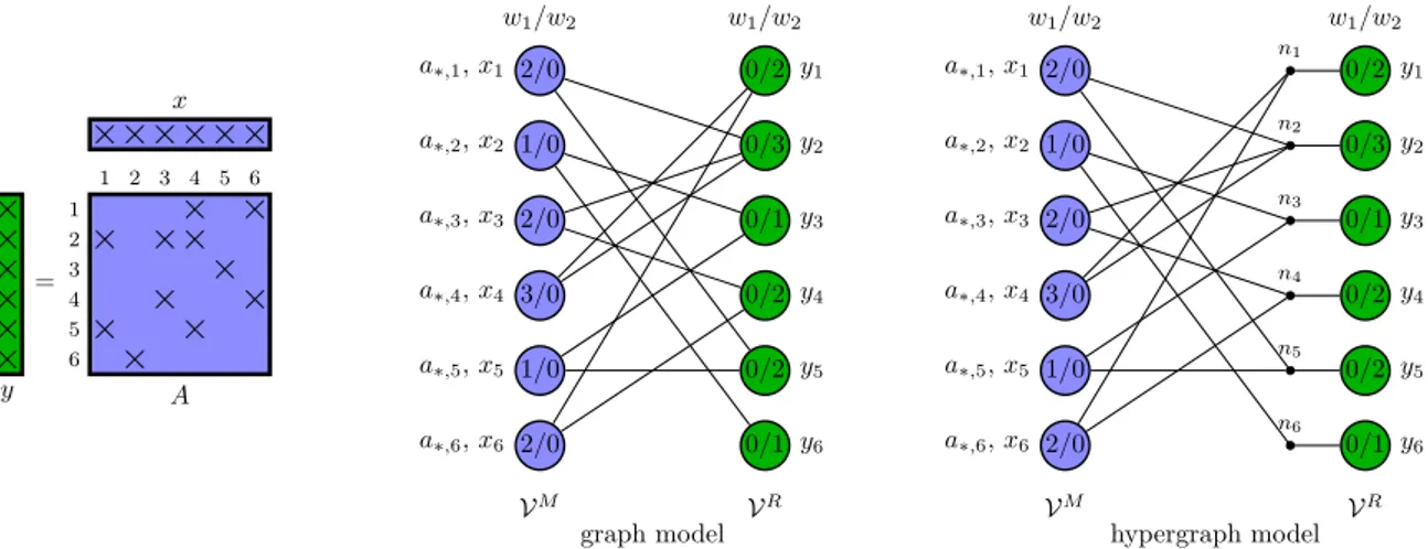
nnz(ai,∗).

The formation and partitioning of the graph/hypergraph for efficient parallelization of column-parallel SpMV in MapReduce framework follow the methodology described in Sections4.1and

4.2, respectively. All edges inGhave unit weights since mj

gen-erates a single KV pair for riif ai,j

̸=

0, and it does not generate

anything, otherwise. All nets inHhave unit costs as well. The K -way partitionsΠM₍_G

_/

_H_{) and}_ΠR₍_G

_/

_H_{) are used to schedule map}

and reduce tasks, details of which will be described in the following section. Fig. 2shows an SpMV operation and its representation with the graph and hypergraph models.

5.2. Implementation

We describe the parallelization of the SpMV operation under MapReduce paradigm. The parallelization is realized using the MR-MPI library [14]. We first give the MapReduce-based paralleliza-tion, and then explain how to assign the tasks to the processors in order to decrease the communication overhead in the shuffle phase and balance the loads of the processors in both map and reduce phases.

Algorithm1presents the MapReduce-based parallelization of SpMV. The SpMV operation is assumed to be repeated in an application-specific context and it is highlighted in gray in the algo-rithm. We omit the application-specific details and focus solely on the SpMV operation itself. Note that a similar routine is also used

(6)

Fig. 2. An example SpMV, and graph and hypergraph models to represent it. The numbers inside the vertices indicate the two weights associated with them. Vectors and

matrices are color-matched with the vertices they are represented with. (For interpretation of the references to color in this figure legend, the reader is referred to the web version of this article.)

in [14] without explicit usage of any hash function. In the algo-rithm, A and x are distributed among the processors via aggregate() operation prior to performing SpMV and they are keyed according to column index j (line 2 and 3). aggregate() operation can take a hash function as input (whose role is going to be clarified shortly). The keys regarding A and x are added to y and they are converted to the KMV pairs (lines 6–8). Then, the multiplication operations are performed via reduce(), in which the multiple values belonging to key j are reduced via multiplying value of each with xj. The results

of this operation are the partial results for y that are keyed by index

i. yj_i denotes the partial value generated by column j for yi. The

operations up to this point constitute the first computational phase of the column-parallel algorithm.

The first computational phase is followed by an optional local reduce in which the partial results are summed locally (note that these summations do not compute the final values of y yet). The partial results are then communicated and KMV pairs are created accordingly, producing possible multiple yj_ivalues for yi(line 12).

Notice that collate() also accepts a hash function as input.

Finally, the partial results are reduced and the final values of y are computed by simply summing them (line 13). The computation of final values constitutes the second computational phase of the column-parallel algorithm. Note that the first computational phase is the ‘‘map’’ phase even though a reduce call has been performed, as it emits KV pairs and is followed by a shuffle phase, which is in turn followed by a reduce operation to compute the final results.

We make use of the partitionsΠM

_{= {}

_VM

1

, . . . ,

V

M

K

}

andΠR

=

{

V₁R

, . . . ,

V_KR

}

described earlier in order to achieve an efficient distribution of data and computations in Algorithm1. ΠM and

ΠR_{can be utilized as hash functions in the algorithm, which are}

respectively denoted with hMand hR. hMis simply obtained from

ΠM_as

hM(j

:

v

jm

∈

VkM)

=

Pk, 1

≤

j

≤

n and 1

≤

k

≤

K

,

which allows distributing matrix columns, elements of x and the respective map tasks via aggregate() with hMas its input. Similarly, hRis obtained fromΠRas

hR(i

:

v

ri

∈

VkR)

=

Pk, 1

≤

i

≤

n and 1

≤

k

≤

K

,

which allows distributing elements of y and the respective reduce tasks on them via collate()1_{with h}

Ras its input.

1_{collate() is actually an aggregate() followed by a con}_v_ert().

6. Sparse matrix-sparse matrix multiplication

The literature on parallelization of sparse matrix-sparse ma-trix multiplication of form C

=

AB (SpGEMM) is more recent

compared to that on SpMV. One of the recent promising studies on this subject is based on parallelization with one-dimensional partitioning of input matrices (A and B) and outer product tasks via hypergraph models [33]. We first briefly review the parallel algorithm for SpGEMM and discuss the graph and hypergraph models in the context of MapReduce framework. Then, we describe the MapReduce implementation of SpGEMM and show how to use the partitions obtained by the graph/hypergraph models to assign map and reduce task to processors.

6.1. Parallel algorithm and MapReduce

We focus on one-dimensional partitioning of input matrices A and B, and two-dimensional partitioning of output matrix C . The matrices A and B are permuted into block structures as

⎡

⎢

⎣

A11

. . .

A1K

... ... ...

AK 1

. . .

AKK

⎤

⎥

⎦

and

⎡

⎢

⎣

B11

. . .

B1K

... ... ...

BK 1

. . .

BKK

⎤

⎥

⎦ ,

respectively, where A is an m

×

n and B is an n

×

p matrix.

Processor Pk is held responsible from the outer products in kth

column stripe Ac

k

= [

AT1k

. . .

ATKk

]

T of A and the respective kth row

stripe Br

k

= [

Bk1

. . .

BkK

]

of B. An outer product performed between

a column x of A and the respective row x of B is denoted with

a∗,x

⊗

bx,∗It is assumed if Pkstores a∗,x, it also stores bx,∗in order

to avoid redundant communication (i.e., a conformal partition of A and B). The described partitions of A and B do not induce a natural partition of C since the outer products performed by a processor may contribute to any nonzero in C . In other words, there is no locality in access to elements of C .

The parallel algorithm that results from the columnwise parti-tioning of A and the rowwise partiparti-tioning of B is called the

outer-product–parallel algorithm for SpGEMM and its basic steps for Pk

are as follows:

1. For each column x in column stripe Ac

k (and hence each

row in row stripe Br

k), Pkcomputes the outer product Cx

=

a∗,x

⊗

bx,∗. This outer product generates partial result(s) for

the elements of C , denoted with Cx. There exists a complete partial result set for each such outer product. Observe that two such different partial result set Cx_{and C}y_{may contain}

(7)

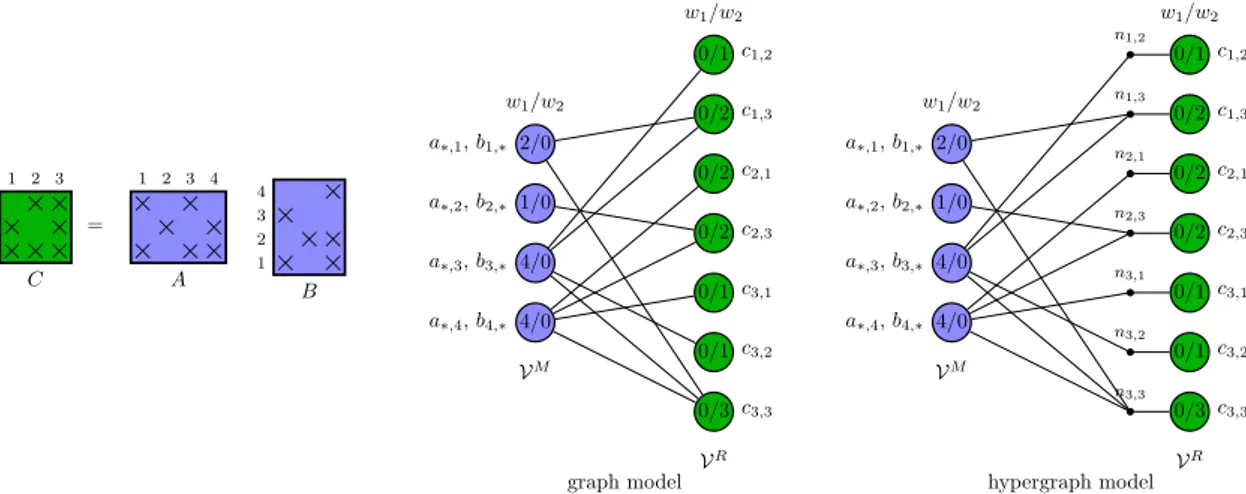
Fig. 3. An example SpGEMM, and graph and hypergraph models to represent it. The numbers inside the vertices indicate the two weights associated with them. Matrices

are color-matched with the vertices they are represented with. (For interpretation of the references to color in this figure legend, the reader is referred to the web version of this article.)

partial results for the same element of C . Pkmay sum them

by

∑

xCxor it may not do so and leave them as they are. If ci,jbelongs to Pk, it sets the initial value of this nonzero by ci,j

=

cik,j.

2. The partial results are communicated to aggregate each c_iℓ_,_j at Pk with the aim of computing the final result of this

nonzero whose accumulation responsibility is given to Pk.

To do so, Pkreceives each such partial result ciℓ,jcomputed

by P_ℓ(

ℓ ̸=

k).

3. In the final step, Pksums the partial results by ci,j

=

ci,j

+

ciℓ,j

for each P_ℓ.

As in the column-parallel SpMV, we assume no overlap of communication and computation and the steps proceed in a sim-ilar manner to the BSP model. Notice the resemblance of outer-product–parallel algorithm for SpGEMM to the column-parallel algorithm for SpMV. The outer-product–parallel SpGEMM has the same skeleton with the column-parallel SpMV, where there exists a single communication phase between two computational phases. Here too the first computational phase is likely to be more expen-sive compared to the second one.

In the parallel algorithm above, there are n map tasks and

nnz(C ) reduce tasks, i.e.,

|

M

| =

n and

|

R

| =

nnz(C ). A map

task mxis defined as the outer product a∗,x

⊗

bx,∗ (performed in

the first step of the outer-product–parallel algorithm). For each

ci,j

∈

Cx, mxgenerates a single KV pair, hence, k

v

p(mx)

= {⟨

ci,j,ai,x

∗

bx,j

⟩ :

ai,x,bx,j

̸=

0 for 1

≤

i

≤

m and 1

≤

j

≤

p

}

. A reduce

task ri,jis defined as the summation of partial results generated

for ci,j(performed in the third step of the outer-product–parallel

algorithm). The KV pairs destined for ri,jis given by k

v

p(ri,j)

= {⟨

ci,j,ai,x

∗

bx,j

⟩ :

ai,x,bx,j

̸=

0 for 1

≤

x

≤

n

}

.

The size of mx is proportional to the number of operations

per-formed in the respective outer product, hence, size(mx)

=

nnz(a∗,x)

×

nnz(bx,∗), whereas the size of ri,jis proportional to the number

of outer products that generate a partial result for ci,j, hence, size(ri,j)

= |{

Cx

:

ci,j

∈

Cx

}|

.

In the graph and hypergraph models used to parallelize the outer-product–parallel SpGEMM in the MapReduce framework, all edges and nets have unit costs, respectively. The K -way partitions

ΠM₍_G

_/

_H_{) and}_ΠR₍_G

_/

_H_{) are used to schedule map and reduce}

tasks, details of which will be described in the following section.

Fig. 3shows an SpGEMM operation and its representation with the

graph and hypergraph models.

Algorithm 2: Sparse matrix-sparse matrix multiplication Input: A

,

B

,

hM

,

hR

1 A.aggregate(hM) ▷ Key x, Value (i,ai,x,‘c’)

2 B.aggregate(hM) ▷ Key x, Value (j,bx,j,‘r’)

3 Let C be an empty MapReduce object 4 repeat ▷other computations... 5 C .add(A) 6 C .add(B) 7 C .convert() ▷ IN Key j, MultiValue[(i,ai,x,‘c’), . . . ,(j,bx,j,‘r’), . . .] 8 C .reduce()

▷ OUT: Key (i,j), Value cx i,j=ai,xbx,j

▷optional local reduce

9 C .convert()

10 C .reduce()

▷communication phase (shuffle)

11 C .collate(hR) ▷ OUT: Key (i,j), MultiValue[cx

i,j]

▷ IN Key (i,j), MultiValue[cx i,j]

12 C .reduce()

▷ OUT Key (i,j), Value∑

xcxi,j

▷other computations...

until application-specific condition is met

6.2. Implementation

We describe the parallelization of the SpGEMM operation un-der MapReduce paradigm. We first give the MapReduce-based parallelization, and then explain how to assign the tasks to the processors in order to decrease the communication overhead in the shuffle phase and balance the loads of the processors in both map and reduce phases.

Algorithm2presents the MapReduce-based parallelization of SpGEMM. The algorithm solely focuses on parallelizing SpGEMM and ignores the application-specific issues. In the algorithm, the matrices A and B are distributed among the processors via

aggregate() operation and matrix A is keyed according to column

(8)

Table 1

Matrices used in the experiments.

Number of Row/column degree Operation Matrix Rows/columns Nonzeros Average Maximum

SpMV y=Ax 333SP 3,712,815 22,217,266 6.0 28 adaptive 6,815,744 27,248,640 4.0 4 circuit5M_dc 3,523,317 19,194,193 5.5 27 CurlCurl_4 2,380,515 26,515,867 11.1 13 delaunay_n23 8,388,608 50,331,568 6.0 28 germany_osm 11,548,845 24,738,362 2.1 13 hugetrace-00000 4,588,484 13,758,266 3.0 3 rajat31 4,690,002 20,316,253 4.3 1252 rgg_n_2_24_s0 16,777,216 265,114,400 15.8 40 Transport 1,602,111 23,500,731 14.7 15 SpGEMM C=AAT crashbasis 160,000 1,750,416 10.9 18 crystm03 24,696 583,770 23.6 27 dawson5 51,537 1,010,777 19.6 33 ia2010 216,007 1,021,170 4.7 49 kim1 38,415 933,195 24.3 25 lhr71 70,304 1,528,092 21.7 63 olesnik0 88,263 744,216 8.4 11 rgg_n_2_17_s0 131,072 1,457,506 11.1 28 struct3 53,570 1,173,694 21.9 27 xenon1 48,600 1,181,120 24.3 27

and 2). The values contained in these keys are the nonzero ele-ments and additional information regarding row/column indices and identification of matrices. C is initially empty and it is filled with the KV pairs of A and B (lines 5 and 6). These pairs are converted to KMV pairs next (line 7). Then, the multiplication operations are performed via reduce(), in which each element of column x of A is multiplied with each element of row x of B, i.e., a∗_,x

⊗

bx,∗. The results of this outer product are the partial

results for C that are keyed with the row and column pair indices,

(i

,

j), in order to achieve a two-dimensional partitioning of C . This

first computational phase is followed by an optional local reduce in which the partial results are summed. Next follows a collate() in which the partial results are communicated and KMV pairs are created accordingly, producing possible multiple cx

i,jvalues for ci,j

(line 11). The final step of SpGEMM corresponds to the second computational phase of the outer-product–parallel algorithm and it contains the reduction of ci,jvia summation (line 12). Observe

that similar to SpMV, the functions aggregate() and collate() take hash functions as their input, which we exploit to achieve task assignments in Algorithm2.

We make use of the partitionsΠM

_{= {}

_VM

1

, . . . ,

VKM

}

andΠR

=

{

V₁R

, . . . ,

V_KR

}

obtained by the graph/hypergraph models and use them as hash functions in order to achieve an efficient distribution of data and computations, as done for SpMV. hMis obtained from

ΠM_as

hM(x

:

v

xm

∈

VkM)

=

Pk, 1

≤

x

≤

n and 1

≤

k

≤

K

,

and hRis obtained fromΠRas

hR((i

,

j)

:

v

ir,j

∈

VkR)

=

Pk, 1

≤

i

≤

m, 1

≤

j

≤

p

and 1

≤

k

≤

K

.

hM is used along with aggregate() to obtain a columnwise

dis-tribution of A, a rowwise disdis-tribution of B and a disdis-tribution of map tasks. hR, on the other hand, is used along with collate() to

obtain a two-dimensional nonzero-based distribution of C and a distribution of reduce tasks.

7. Experiments

We test a total of six schemes in our experiments:

• RN

: The tasks in the first and the second computation phases are distributed among the processors in a random manner

and local reduce is not performed (i.e., lines 10 and 11 in Algorithm1and lines 9 and 10 in Algorithm2are not exe-cuted). This scheme is equivalent to using the default hash function in the MapReduce implementation in Algorithms1

and2for aggregating data.

• RNr

: Similar to

RN

, but with the optional local reduce.

• GR

: The tasks in the first and the second computation phases are distributed among the processors with the graph models with the aim of decreasing communication overhead under the load balance constraint. Local reduce is not performed in this scheme.

• GRr

: Similar to

GR

, but with the optional local reduce.

• HY

: The tasks in the first and the second computation phases are distributed among the processors with the hypergraph models with the aim of decreasing communication over-head under the load balance constraint. Local reduce is not performed in this scheme.

• HYr

: Similar to

HY

, but with the optional local reduce. The experiments are performed on an IBM System x iData-Plex machine (dx360M4). A node on this machine consists of 16 cores (two 8-core Intel Xeon E5 processors) with 2.7 GHz clock frequency and 32 GB memory. The nodes are connected with an Infiniband non-blocking tree network topology. We tested for 32

,

64

, . . . ,

1024 processors. Recall that these are also the number of parts in partitioning models.

All sparse matrix operations (SpMV, SpGEMM) are imple-mented using the MR-MPI library [14]. The partitions obtained by the graph/hypergraph models are fed to the aggregate() and

collate() as hash functions. Each sparse matrix operation is

re-peated 10 times and the average is reported in the results in the upcoming sections. Metis [34] is used to partition the graphs and PaToH [32] is used to partition the hypergraphs, both in default settings. The maximum allowed imbalance in processors’ loads in both computational phases is set to 10% for each of the two constraints. Recall that this imbalance determines the maximum allowed imbalance in both computational phases.

We evaluate the performance of all schemes for each operation with the matrices given inTable 1, which are from the UFL Sparse Matrix Collection [35]. For each type of operation, we include 10 matrices. The maximum degree values presented in the table are the maximum of maximum number of nonzeros in rows and columns. For SpGEMM, we test the operation C

=

AAT_{, which}

(9)

Table 2

Volume, imbalance and runtime averages for SpMV (volume in megabytes and time in seconds).

Actual values Normalized within scheme Normalized wrtRNandRNr

K Scheme RNr RN GRr GR HYr HY RN/RNr GR/GRr HY/HYr GRr/RNr HYr/RNr GR/RN HY/RN

32 %imb-map 0.5 0.5 0.7 0.7 0.9 0.9 1.00 1.00 1.00 1.4 2.0 1.4 2.0 %imb-reduce 0.5 0.5 1.0 1.0 1.6 1.6 1.00 1.00 1.00 1.9 3.2 1.9 3.2 volume 406.3 448.9 0.6 1.0 0.5 1.6 1.10 1.60 2.91 0.002 0.001 0.002 0.004 time 1.26 0.93 0.61 0.59 0.61 0.60 0.74 0.96 0.99 0.49 0.48 0.64 0.65 64 %imb-map 0.8 0.8 1.6 1.6 0.9 0.9 1.00 1.00 1.00 2.1 1.2 2.1 1.2 %imb-reduce 0.7 0.7 2.1 2.1 2.0 2.0 1.00 1.00 1.00 2.9 2.7 2.9 2.7 volume 433.7 456.2 0.9 1.5 0.8 2.4 1.05 1.59 2.88 0.002 0.002 0.003 0.005 time 0.64 0.47 0.33 0.32 0.33 0.32 0.74 0.97 0.97 0.52 0.52 0.69 0.68 128 %imb-map 1.0 1.0 3.2 3.2 1.3 1.3 1.00 1.00 1.00 3.1 1.2 3.1 1.2 %imb-reduce 1.2 1.2 3.6 3.6 2.7 2.7 1.00 1.00 1.00 2.9 2.2 2.9 2.2 volume 448.5 459.9 1.4 2.2 1.2 3.5 1.03 1.59 2.84 0.003 0.003 0.005 0.008 time 0.34 0.25 0.20 0.18 0.20 0.19 0.71 0.91 0.93 0.59 0.59 0.75 0.76 256 %imb-map 1.6 1.6 4.2 4.2 1.6 1.6 1.00 1.00 1.00 2.7 1.0 2.7 1.0 %imb-reduce 2.0 2.0 5.3 5.3 3.6 3.6 1.00 1.00 1.00 2.6 1.8 2.6 1.8 volume 455.9 461.7 2.0 3.1 1.8 5.0 1.01 1.58 2.76 0.004 0.004 0.007 0.011 time 0.20 0.15 0.13 0.12 0.13 0.12 0.73 0.89 0.89 0.66 0.67 0.81 0.81 512 %imb-map 2.7 2.7 6.0 6.0 1.9 1.9 1.00 1.00 1.00 2.2 0.7 2.2 0.7 %imb-reduce 3.3 3.3 7.4 7.4 5.1 5.1 1.00 1.00 1.00 2.2 1.5 2.2 1.5 volume 459.7 462.6 2.9 4.5 2.6 7.1 1.01 1.57 2.71 0.006 0.006 0.010 0.015 time 0.17 0.13 0.10 0.09 0.10 0.09 0.78 0.86 0.86 0.60 0.60 0.66 0.66 1024 %imb-map 3.9 3.9 7.1 7.1 2.2 2.2 1.00 1.00 1.00 1.8 0.6 1.8 0.6 %imb-reduce 4.5 4.5 8.8 8.8 6.6 6.6 1.00 1.00 1.00 1.9 1.5 1.9 1.5 volume 461.7 463.1 4.1 6.4 3.8 10.1 1.00 1.56 2.68 0.009 0.008 0.014 0.022 time 0.23 0.19 0.09 0.07 0.09 0.07 0.85 0.83 0.82 0.39 0.40 0.38 0.39

is also listed as one of the key operations and included in the experiments of [33].

7.1. SpMV

The results obtained for the SpMV operation are presented

inTable 2. We compare the schemes in terms of four metrics:

computational imbalance in map and reduce phases in terms of KV pairs (indicated with imb-map and imb-reduce, respectively), communication volume (volume) and runtime (time). The volume is in terms of megabytes (Mb) and the time is in terms of seconds. The table is grouped under three basic column groups. The first column group presents the actual results obtained by the com-pared schemes. The second column group compares the schemes within themselves, i.e., with and without the optional local reduce. The last column group measures the performance of partitioning models against the baseline random assignment. Each value in the table is the geometric mean of the results obtained for the matrices used for SpMV on a specific number of processors. The last two column groups contain the normalized values in the format of A

/

B,

which means scheme A is normalized with respect to scheme B. When we compare the schemes that use partitioning models for task assignment (i.e.,

GR

,

GRr

,

HY

,

HYr

) against the ones that do not (i.e.,

RN

,

RNr

), the benefits of using a model are seen clearly. These models decrease the communication volume drastically by obtaining a volume of no more than 7 Mb in any K value, whereas the communication volume of

RN

or

RNr

is around 400 Mb. The reduction in communication volume is reflected as improvement in overall runtime of the SpMV. For example on 128 processors,

RN

obtains an SpMV time of 0.34 s, while

GR

obtains an SpMV time of 0.18 s. In terms of imbalance, the schemes that utilize random assignment usually exhibit better performance since the sole pur-pose of these schemes is maintaining such a balance, while for the schemes that utilize partitioning models balance is a constraint rather than objective.

The execution of the optional local reduce is expected to de-crease the communication volume. This is validated from the val-ues in the second column group and the volume row. For example on 128 processors,

RN

incurs 3% more volume than

RNr

,

GR

incurs

59% more volume than

GRr

and

HY

incurs 184% more volume than

HYr

. This difference is less in

RN

and

RNr

since random assignment already necessitates a large amount of communication. The results regarding the optional local reduce indicate that performing local reduce does not pay off as the parallel runtimes obtained by

RN

,

GR

and

HY

are lower than the ones obtained by

RNr

,

GRr

and

HYr

, respectively. However, this may not always be the case, especially when the savings from communication are drastic with the execu-tion of local reduce, which happens not to be the case for SpMV. Note that the imbalances in KV pairs in the first and second phases of computations are the same with or without the local reduce as their counts are independent of it.

Recall that without the local reduce, the graph model correctly encapsulates the total volume during the partitioning process. From the volume results inTable 2, when we compare

GR

and

HY

, it is seen that

GR

obtains lower volume for any K : for example on 512 processors the volume of

GR

is 4.5 Mb while it is 7.1 Mb for

HY

. On the other hand, with the local reduce, the hypergraph model correctly encapsulates the total volume. When we compare

GRr

and

HYr

, it is seen that

HYr

obtains lower volume for any K : for example on 512 processors the volume of

HYr

is 2.6 Mb while it is 2.9 Mb for

GRr

.

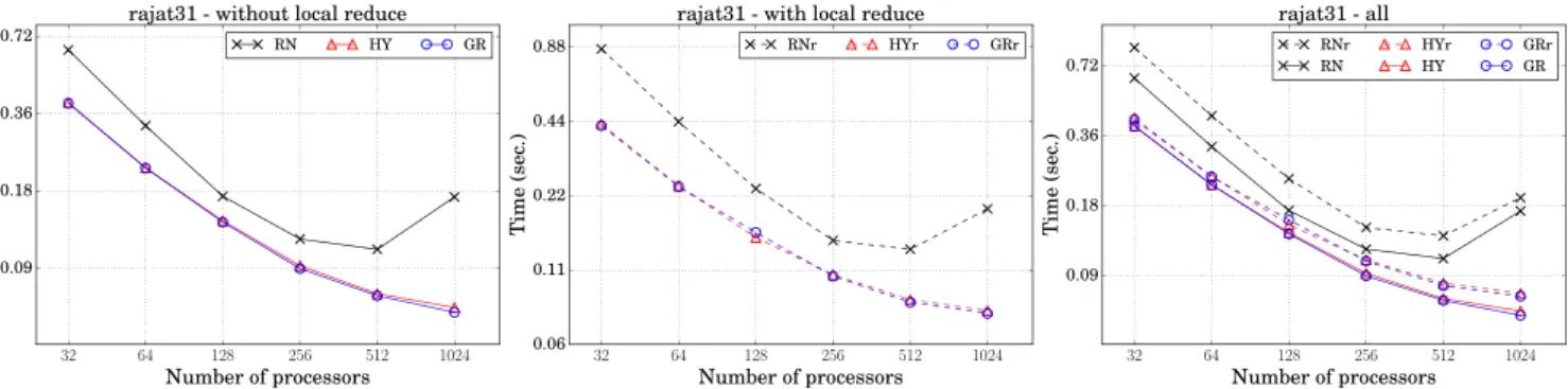
Fig. 4 presents the parallel SpMV runtimes obtained by the

compared schemes for matrix

rajat31

. There are three plots: the one in the left compares the schemes that do not contain local reduce, i.e.,

RN

,

GR

,

HY

, the one in the center compares the schemes that contain local reduce, i.e.,

RNr

,

GRr

,

HYr

, and the one in the right compares all. We display the plots for a single matrix only as the plots for other matrices exhibit similar behaviors. Both with and without local reduce, the task assignments realized by the partitioning models scale much better. Observe that the schemes without local reduce obtain lower runtimes compared to their counterparts, as also observed inTable 2. Up to 256 processors, all schemes seem to scale, but after that point, the schemes relying on random assignment scale poorly while the schemes relying on partitioning models scale further by being able to decrease the runtime. The reason behind this is the increased importance of communication in overall runtime, which we investigate next.

Fig. 5illustrates the dissection of parallel SpMV times as bar

(10)

Fig. 4. Parallel SpMV runtimes of compared schemes for matrixrajat31. Both axes are in logarithmic scale.

Fig. 5. Dissection of computation and communication times in parallel SpMV for matrixrajat31on 32, 128 and 512 processors. (For interpretation of the references to color in this figure legend, the reader is referred to the web version of this article.)

and yellow bars in the figure respectively represent the compu-tation and communication times. When we compare the perfor-mance of different schemes (

RNr

,

GRr

,

HYr

) for a specific number of processors with local reduce, it is seen that the computation times are roughly the same, whereas the communication times vary drastically. This is also the case without local reduce. When we compare the communication performance of a scheme for a specific number of processors, it is observed that local reduce decreases the communication time significantly as expected. Al-though it is expected that the total amount of computation of a scheme for a specific number of processors should stay the same with or without local reduce, this does not seem to be the case due to the overhead of the con

v

ert() and reduce() operations involved

in local reduce. As seen from both bar charts, the key to scalability is to address the communication bottlenecks, which is achieved by the partitioning models in a very successful manner.

7.2. SpGEMM

The results obtained for the SpGEMM operation are presented

in Table 3. The decoding of the table is the same with the one

presented for SpMV (Table 2). We experiment up to 512 processors for this operation.

As seen fromTable 3, the schemes that utilize a partitioning model decrease the communication volume drastically in the shuf-fle phase. For example on 128 processors,

GRr

and

HYr

incur a volume of 5–6 Mb, while

RNr

incurs a volume of 341.7 Mb. Sim-ilarly, on the same number of processors,

GR

and

HY

respectively incur a volume of 13.1 and 21.4 Mb, while

RN

incurs a volume of 356 Mb. The benefit of decreasing data transferred is seen as improvement in parallel SpGEMM runtime: the schemes relying on partitioning models obtain more than 2-4x speedup over the

ones that do not so for any number of processors. The schemes exhibit close performance in computational balance in the map phase. However,

RN

and

RNr

obtain better balance in the reduce phase.

As also observed in the SpMV operation, performing the op-tional local reduce leads to reductions in data transfer in the shuffle phase. For random assignment schemes, the optional local reduce does not seem to work as

RNr

obtains higher parallel SpGEMM times than

RN

. This is because there is not much difference in the volumes incurred by these two schemes. On the other hand, for small number of processors, the optional local reduce pays off for the schemes that rely on partitioning models up to 256 processors. Comparing the volumes incurred by the graph and hypergraph models, when there is no local reduce

GR

always obtains lower volume than

HY

for any number of processors. In the existence of local reduce,

HYr

obtains lower volume than

GRr

for 128, 256 and 512 processors, while

GRr

obtains lower volume than

HYr

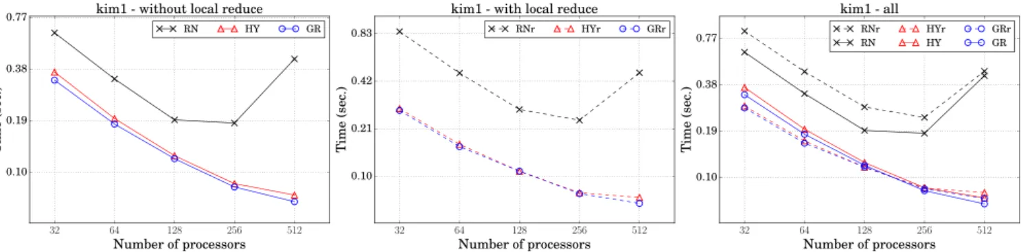
in 32 and 64 processors. Note that graph partitioners can perform close to hypergraph partitioners if the sparsity pattern of the underlying model accommodates uniformity.

Fig. 6presents the parallel SpGEMM runtimes obtained by the

compared schemes for matrix

kim1

. The left plot compares the schemes that do not contain local reduce, i.e.,

RN

,

GR

,

HY

, the center plot compares the schemes that contain local reduce, i.e.,

RNr

,

GRr

,

HYr

, and the right plot compares all. With or without local reduce, the schemes relying on partitioning models exhibit better scalability.

RN

and

RNr

scale up to 128 processors, while

GR

,

GRr

,

HY

and

HYr

scale all the way up to 512 processors. As also observed

inTable 3,

GRr

and

HYr

perform slightly better than

GR

and

HY

on small number of processors, while the opposite situation is observed on 256 and 512 processors.

(11)

Table 3

Volume, imbalance and runtime averages for SpGEMM (volume in megabytes and time in seconds).

Actual values Normalized within scheme Normalized wrtRNandRNr

K Scheme RNr RN GRr GR HYr HY RN/RNr GR/GRr HY/HYr GRr/RNr HYr/RNr GR/RN HY/RN

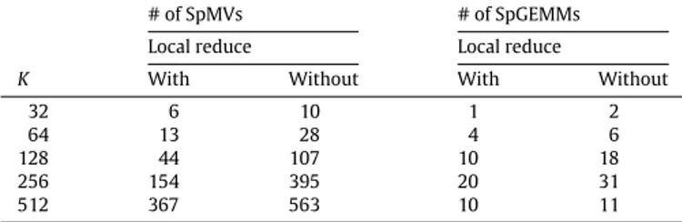
32 %imb-map 6.5 6.5 7.3 7.3 5.6 5.6 1.00 1.00 1.00 1.1 0.9 1.1 0.9 %imb-reduce 0.6 0.6 4.9 4.9 2.9 2.9 1.00 1.00 1.00 7.8 4.7 7.8 4.7 volume 299.7 347.6 2.2 4.4 2.4 10.1 1.16 2.00 4.28 0.007 0.008 0.013 0.029 time 0.76 0.57 0.30 0.32 0.31 0.36 0.75 1.08 1.17 0.39 0.41 0.56 0.63 64 %imb-map 9.1 9.1 10.4 10.4 9.0 9.0 1.00 1.00 1.00 1.2 1.0 1.2 1.0 %imb-reduce 0.9 0.9 7.2 7.2 4.5 4.5 1.00 1.00 1.00 7.7 4.8 7.7 4.8 volume 326.4 353.1 3.6 7.0 3.8 15.2 1.08 1.97 4.00 0.011 0.012 0.020 0.043 time 0.43 0.33 0.17 0.18 0.18 0.21 0.75 1.04 1.11 0.40 0.42 0.56 0.63 128 %imb-map 17.5 17.5 15.4 15.4 12.9 12.9 1.00 1.00 1.00 0.9 0.7 0.9 0.7 %imb-reduce 1.3 1.3 10.1 10.1 5.8 5.8 1.00 1.00 1.00 8.0 4.6 8.0 4.6 volume 341.7 356.0 6.1 13.1 5.7 21.4 1.04 2.15 3.73 0.018 0.017 0.037 0.060 time 0.25 0.19 0.12 0.11 0.12 0.12 0.73 0.99 1.02 0.45 0.48 0.61 0.66 256 %imb-map 20.0 20.0 23.4 23.4 18.0 18.0 1.00 1.00 1.00 1.2 0.9 1.2 0.9 %imb-reduce 2.0 2.0 15.9 15.9 8.2 8.2 1.00 1.00 1.00 8.0 4.2 8.0 4.2 volume 350.1 357.4 9.6 21.7 8.8 32.2 1.02 2.26 3.65 0.027 0.025 0.061 0.090 time 0.18 0.14 0.09 0.08 0.09 0.09 0.77 0.92 0.97 0.49 0.50 0.58 0.63 512 %imb-map 30.1 30.1 29.3 29.3 24.7 24.7 1.00 1.00 1.00 1.0 0.8 1.0 0.8 %imb-reduce 3.9 3.9 18.3 18.3 12.9 12.9 1.00 1.00 1.00 4.7 3.3 4.7 3.3 volume 354.4 357.8 14.2 32.4 13.4 46.8 1.01 2.28 3.49 0.040 0.038 0.091 0.131 time 0.30 0.27 0.07 0.06 0.08 0.07 0.90 0.87 0.89 0.24 0.25 0.24 0.25 Table 4 Amortization of partitioning. # of SpMVs # of SpGEMMs Local reduce Local reduce

K With Without With Without

32 6 10 1 2

64 13 28 4 6

128 44 107 10 18

256 154 395 20 31

512 367 563 10 11

Fig. 7illustrates the dissection of parallel SpGEMM times as bar

charts for matrix

kim1

on 32, 128 and 512 processors. Observe that, as also was the case for SpMV, the schemes with local reduce have less communication overhead compared to the schemes without local reduce. The arguments made for SpMV are also valid for SpGEMM. Compared to SpMV, the improvements in the commu-nication performance are more pronounced with the execution of the local reduce. This is due to the higher number of intermediate KV pairs produced in SpGEMM. Since all schemes achieve a good computational balance, the key to better parallel performance and scalability lies in the reduction of communication overheads.

7.3. Preprocessing and amortization

We evaluate the pre-processing overheads of the proposed models inTable 4. We only consider the schemes based on graph partitioning, i.e.,

GR

and

GRr

, in our analyses to compare with

RN

and

RNr

due to a number of reasons. First, graph partition-ing is faster compared to hypergraph partitionpartition-ing and when the close performance of graph and hypergraph models is taken into account,

GR

and

GRr

become more viable compared to

HY

and

HYr

in terms of pre-processing overhead. Second, while there exist several fast parallel partitioners for graphs, this is not the case for hypergraphs. Hence, the analyses in this section do not involve

HY

and

HYr

. InTable 4, an entry signifies the number of SpMV or SpGEMM iterations required to amortize the partitioning overhead and is the geometric average of the matrices used for the respective operation and K value. For example, the value of 44 in the table indicates that compared to

RNr

, partitioning the graphs and running SpMV in parallel using

GRr

amortizes

GRr

’s partitioning overhead in 44 SpMV iterations. We use ParMETIS [36] to partition the graphs.

From the values in Table 4, it is clearly seen that the graph models for SpGEMM amortize much better than the graph models for SpMV. For example, for K

=

128, while 44–107 iterations are required for SpMV to amortize, only 10–18 iterations are required for SpGEMM to amortize. This is simply because the graphs for SpGEMM are partitioned faster with ParMETIS compared to the graphs for SpMV.

Another important point is that the graph models amortize better in the existence of local reduce. The reason behind this does not lie in runtime differences between

GR

and

GRr

, which are very close, but between

RN

and

RNr

, which are quite distant especially at small processor counts. The high parallel runtimes of

RNr

compared to that of

RN

(seeTables 2and3), for example, lead

GRr

to amortize in 44 and 10 SpMV and SpGEMM iterations, respectively, at K

=

128, while, these values are 107 and 18 for

GR

. The amortization tends to slow down with increasing number of processors. The reason behind this is that ParMETIS does not scale after a certain number of processors and actually further scales down, where this scaling down is seemingly sharper in SpMV than SpGEMM. This trend seems to evaporate when increas-ing number of processors from 256 to 512, especially for SpGEMM. This is not because ParMETIS miraculously starts scaling up after a certain point, but because

RN

and

RNr

starts to scale down around 256 processors, which in turn decreases the amortization overhead at 512 processors as

GR

and

GRr

scale successfully at any number of processors.

All in all, it can be said that the amortization happens somewhat fast, often not in the magnitudes of tens of hundreds or a few thousands of iterations as expected from an application arising from scientific computing. This is due to the BSP nature of the MapReduce implementation and the HPC nature of the graph par-titioner ParMETIS, the former containing synchronization burdens once every a few operations for the ease of programming while the latter carries no such burdens at the expense of utilizing more complex algorithms.

8. Conclusions

In this work we focused on static scheduling of map and reduce tasks in a MapReduce job to achieve data locality and load bal-ance, where the data locality usually translates into reduced data transfer in the shuffle phase and the load balance usually translates into faster task execution in the map and reduce phases. Our

(12)

Fig. 6. Parallel SpGEMM runtimes of compared schemes for matrixkim1. Both axes are in logarithmic scale.

Fig. 7. Dissection of computation and communication times in parallel SpGEMM for matrixkim1on 32, 128 and 512 processors. (For interpretation of the references to color in this figure legend, the reader is referred to the web version of this article.)

approach relies on exploiting the domain-specific knowledge with the help of the models based on graph and hypergraph partitioning. This knowledge is obtained through scanning the input data in a preprocessing stage to determine the interactions among map and reduce tasks. In order to utilize our models within MapReduce, the information produced by them are used as hash functions to schedule the tasks in map and reduce phases. Our models’ capa-bilities are demonstrated on two key operations, sparse matrix– vector multiplication (SpMV) and sparse matrix-sparse matrix multiplication (SpGEMM) — both of which are common operations in scientific computations and graph algorithms. Using our models in the experiments that contain up to 1024 processors, the amount of data transferred in the shuffle phase has been reduced from several hundreds of megabytes to only a few megabytes, resulting in up to 2.6x speedup for SpMV and 4.2x speedup for SpGEMM.

As future work, we plan to integrate our models into more common dialects of MapReduce such as Hadoop and test them on commodity clusters. Since our models completely ignore the important issues such as fault tolerance in MapReduce, we also plan to investigate methods that will render the proposed models fault-tolerant. Lastly, we consider validating the impact of static task scheduling in more realistic scenarios via models constructed on the fly while running a MapReduce job.

Acknowledgment

We acknowledge PRACE (Partnership for Advanced Computing In Europe) for awarding us access to SuperMUC based in Germany at Leibniz Supercomputing Centre.

References

[1] J. Dean, S. Ghemawat, MapReduce: Simplified data processing on large clusters, Commun. ACM 51 (1) (2008) 107–113.http://dx.doi.org/10.1145/ 1327452.1327492. URL.http://doi.acm.org/10.1145/1327452.1327492. [2] Apache Hadoop.http://hadoop.apache.org/. (Accessed: 2017-01-3). [3] M. Hammoud, M.S. Rehman, M.F. Sakr, Center-of-gravity reduce task

schedul-ing to lower mapreduce network traffic, in: 2012 IEEE Fifth International Conference on Cloud Computing, 2012, pp. 49–58.http://dx.doi.org/10.1109/ CLOUD.2012.92.

[4] B. Palanisamy, A. Singh, L. Liu, B. Jain, Purlieus: Locality-aware resource allo-cation for MapReduce in a cloud, in: Proceedings of 2011 International Con-ference for High Performance Computing, Networking, Storage and Analysis, SC ’11, ACM, New York, NY, USA, 2011, pp. 58:1–58:11.http://dx.doi.org/10. 1145/2063384.2063462. URL.http://doi.acm.org/10.1145/2063384.2063462. [5] S. Ibrahim, H. Jin, L. Lu, S. Wu, B. He, L. Qi, Leen: Locality/fairness-aware key

partitioning for mapreduce in the cloud, in: 2010 IEEE Second International Conference on Cloud Computing Technology and Science, 2010, pp. 17–24. http://dx.doi.org10.1109/CloudCom.2010.25.

[6] M. Hammoud, M.F. Sakr, Locality-Aware reduce task scheduling for mapre-duce, in: Proceedings of the 2011 IEEE Third International Conference on Cloud Computing Technology and Science, CLOUDCOM ’11, IEEE Computer Society, Washington, DC, USA, 2011, pp. 570–576.http://dx.doi.org/10.1109/ CloudCom.2011.87.

[7] M. Liroz-Gistau, R. Akbarinia, D. Agrawal, E. Pacitti, P. Valduriez, Data parti-tioning for minimizing transferred data in mapreduce, in: A. Hameurlain, W. Rahayu, D. Taniar (Eds.), Data Management in Cloud, Grid and P2P Systems: 6th International Conference, Globe 2013, Prague, Czech Republic, August 28-29, 2013. Proceedings, Springer Berlin Heidelberg, Berlin, Heidelberg, 2013, pp. 1–12. URL.http://dx.doi.org/10.1007/978-3-642-40053-7_1.

[8] J. Li, J. Wu, X. Yang, S. Zhong, Optimizing mapreduce based on local-ity of k-v pairs and overlap between shuffle and local reduce, in: 2015 44th International Conference on Parallel Processing, 2015, pp. 939–948. http://dx.doi.org/http:/dx.doi.org/10.1109/ICPP.2015.103.

[9] L. Fan, B. Gao, X. Sun, F. Zhang, Z. Liu, Improving the load balance of mapreduce operations based on the key distribution of pairs, CoRR abs/1401.0355 (2014). URL.http://arxiv.org/abs/1401.0355.