Scheduling with tool changes to minimize total completion time: a study of heuristics and their performance

Time: A Study of Heuristics and Their Performance

1

Department of Industrial Engineering, Bilkent University, 06533 Bilkent, Ankara Turkey 2

Department of Operations Management and Business Statistics, Sultan Quaboos University, Oman

Received 10 June 1999; revised 12 June 2001; accepted 16 May 2002 DOI 10.1002/nav.10045

Abstract: The machine scheduling literature does not consider the issue of tool change. The parallel literature on tool management addresses this issue but assumes that the change is due only to part mix. In practice, however, a tool change is caused most frequently by tool wear. That is why we consider here the problem of scheduling a set of jobs on a single CNC machine where the cutting tool is subject to wear; our objective is to minimize the total completion time. We first describe the problem and discuss its peculiarities. After briefly reviewing available theoretical results, we then go on to provide a mixed 0 –1 linear programming model for the exact solution of the problem; this is useful in solving problem instances with up to 20 jobs and has been used in our computational study. As our main contribution, we next propose a number of heuristic algorithms based on simple dispatch rules and generic search. We then discuss the results of a computational study where the performance of the various heuristics is tested; we note that the well-known SPT rule remains good when the tool change time is small but deteriorates as this time increases and further that the proposed algorithms promise significant improvement over the SPT rule.© 2002 Wiley Periodicals, Inc. Naval Research Logistics 50: 15–30, 2003.

1. INTRODUCTION

It is widely recognized that there is an increasing need today for manufacturing firms to achieve a diverse, small-lot production capability in order to compete in the world market. Computer Numerical Control (CNC) is one form of programmable automation that efficiently accommodates product variations and thus supports the above capability. In this paper, we focus on a single CNC machine (one that is perhaps the bottleneck in a flexible manufacturing system) and address the problem of scheduling a set of jobs on this machine such that their total completion time is minimized. In so doing, we also take into account the disruptions caused by tool changes that are inevitable due to tool wear. This aspect of our work, where we attempt to combine tool management with scheduling, makes it interesting.

Tool management has been acknowledged to be an important issue in manufacturing. Gray, Seidmann, and Stecke [7] and Veeramani, Upton, and Barash [20], in their surveys on tool

Correspondence to: M. S. Akturk

management in automated manufacturing systems, emphasize that the lack of tool management considerations often results in the poor performance. Kouvelis [9] similarly reports that tooling costs can account for 25–30% of both fixed and variable costs of production; also see Tomek [19].

Despite this importance, the scheduling literature has ignored the impact of tool changes, particularly those induced by tool wear. This is striking because Flanders and Davis [6] conclude, from their simulation study of a flexible manufacturing system at Caterpillar, that the failure of the existing scheduling models to consider the constraints arising out of tool changes (as induced by tool wear) can lead to infeasible solutions. The parallel literature on tool management, on the other hand, considers tool changes but assumes that such changes are necessitated only by product mix considerations. This is also striking because Gray, Seidmann, and Stecke [7] note that tools lives are generally short relative to the planning horizon and that tool changes due to tool wear are ten times as frequent as those due to part mix. One exception in the tool management literature where tool wear and tool change issues receive active consideration is perhaps the work of Akturk and Avci [2], who propose a new methodology for jointly determining optimal machining conditions and tool allocation; they, however, do not address the scheduling dimension.

As we have noted above, in much of the tool management literature, tool changes are considered to be due to part mix (i.e., due to the different tooling requirements of the parts). A general overview of problems and solution methods related to tool management is given by Crama [5]. In the tool management studies, cost terms related to scheduling decisions (such as those involving job completion times) are not included in the objective function. The models are mostly motivated by past industrial experience that the time needed for interchanging tools overwhelmingly dominates the job processing times. Thus, the emphasis is on the minimization of the number of tool switches. Tang and Denardo [17] study the single machine case with given tool requirements where tool changes are required due to part mix; they provide heuristic algorithms for job scheduling in this environment and an optimal procedure (viz., the common-sense Keep Tool Needed Soon rule) for a fixed job sequence. They also study the case of parallel tool switchings in a companion paper [18] with the objective of minimizing the number of switching instants. Among others, in one of the earliest efforts, Stecke [15] formulates the tool loading problem as a nonlinear mixed integer programming problem.

However, with new technology, tool change times on CNC machines have been reduced considerably, and thus job processing times are not always significantly dominated by tool change times. For this reason, while scheduling a given set of jobs, considering only tool switches may not result in good solutions with respect to standard scheduling measures such as those involving job completion times.

Turning now to the scheduling literature, it appears that tool changes have not been considered at all. There are, however, a few studies that allow for machine unavailability, which bear similarity to scheduling with tool changes. To the contrary, it is traditional to assume that the machine is capable of continuous processing at all times. This is not very realistic since tools have limited lives and processing has to be interrupted when they wear out. We have already noted that tool wear is quite common and frequent.

The research on scheduling with machine availability constraints, which is related to our work, focuses mostly on machine breakdowns and maintenance intervals. A typical objective is the minimization of the total completion time. Adiri et al. [1] consider, for the first time, the flowtime scheduling problem when the machine faces breakdowns at stochastic time epochs, the repair time is stochastic, but the processing times are constant. They prove that the problem is NP-hard and show that the Shortest Processing Time (SPT) first rule minimizes the expected

total flow time if the time to breakdown is exponentially distributed. Lee and Liman [10] study the deterministic equivalent of this problem in the context of a single scheduled maintenance. They give a simpler proof of NP-hardness and find a tight performance bound of 9/7 for the SPT rule. Lee and Liman [11] also consider the scheduling problem of minimizing total completion time with two parallel machines where one machine is always available and the other is available from time zero up to a fixed point in time. They give the NP-hardness proof for the problem and provide a pseudo-polynomial dynamic programming solution. Lee [12] studies the problem of minimizing makespan in a two-machine flow shop where the availability constraint applies to one machine. In a companion paper, Lee [13] analyzes the scheduling problem with the machine availability constraint in detail, giving results for various performance measures such as makespan, total weighted completion time, total tardiness and number of tardy jobs in single-machine, parallel-machines, and 2-machine flowshop environments.

However, all of the above studies assume a single breakdown or a single maintenance interval and that the interval is of either random or constant duration. But, in scheduling with tool changes, this is not a reasonable assumption as there can be several tool changes over a given time period and the time between tool changes (while bounded by the tool life) can vary. Recently, Qi, Chen, and Tu [14] has considered scheduling with multiple maintenance intervals of variable duration. Their model turns out to be equivalent to ours and leads to the same theoretical results reported by us elsewhere [3]. We point out that variable intervals do not apply to scheduled maintenance where the maintenance activity is performed by a specialized crew at fixed intervals; variable intervals may only apply to routine maintenance performed by the machine operator (such as cleaning, lubricating, and adjusting). We provide here our treatment of the single-machine scheduling problem where processing is interrupted due to tool wear and tool changes and the objective is to minimize the total job completion time.

The rest of the paper is organized as follows. We first describe the problem and discuss its peculiarities. We then briefly summarize the available theoretical results; we go on to describe a mixed 0 –1 programming formulation for the exact solution of the problem, which is used by us in solving small problem instances. As our main thrust, we next propose a number of heuristic algorithms based on simple dispatch rules and generic search; these algorithms are then illustrated through the use of a numerical example. At this point, we also present and discuss the results of a computational study undertaken by us to evaluate the absolute/relative performance of the various heuristics. Finally, we close with a brief summary of our work and a few remarks.

2. PROBLEM DESCRIPTION AND DISCUSSION

We are given a single CNC machine that is continuously available (except when undergoing a tool change) and n independent jobs that are ready for processing at time zero. The job processing times are constant and known a priori. Only one type of tool with a known, constant life and an unlimited availability is required. (The use of one tool type is not unusual in practice as illustrated by the case of CNC drills.) When an active tool wears out, it is replaced with a new one; the time needed for this tool change is also known and constant. We do not allow the processing of a job to be interrupted because of a tool change or otherwise in order to achieve the desired surface-finish.

Under the above circumstances, we wish to find a schedule that will minimize the total completion time of the jobs. We see that it is not to our advantage to have any machine idle time other than what is forced by a tool change or to change a tool when it can process the job that is next in sequence. Thus, a job sequence translates uniquely to a schedule and a tool allocation.

We will use the terms sequence and schedule interchangeably. The notation used throughout the paper is now introduced:

TL⫽ tool life,

TC⫽ tool change time,

pi⫽ processing time of job i (assume w.l.o.g. that the jobs are numbered in the SPT order and that pi ⱕ TL),

p[k]⫽ processing time of job at position k in some schedule, Ci⫽ completion time of job i in some schedule,

tj⫽ sum of processing times of jobs using the jth tool in some schedule, ␩j␴⫽ number of jobs allocated to the jth tool in schedule␴,

K_␴⫽ number of tools used by schedule␴, Z_␴⫽ the total job completion time of schedule␴, Z1␴⫽ the contribution of the job processing times to Z␴, Z2␴⫽ the contribution of tool change times to Z␴.

Minimizing the total completion time is one of the basic objectives studied in the scheduling literature. It is well known that the SPT dispatching rule will give an optimal schedule in the single machine case if the tool life is considered infinitely long (i.e., there is no tool change). However, the structure of the problem changes dramatically when we introduce tool changes. Depending upon the value of TC, the SPT rule may or may not perform well. Note that the SPT rule in the present context will assign jobs to successive tools in nondecreasing order of their processing times and change tools when a job cannot be accommodated on the current tool.

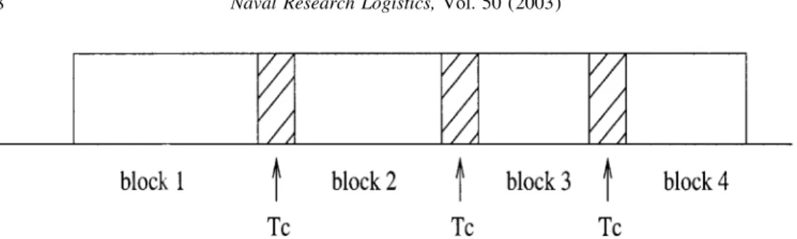
If we consider the jobs sharing the same tool as a block, a schedule can be viewed as blocks of jobs separated by tool changes (see Fig. 1); this representation is useful in describing a schedule. Note that the length of the blocks do not have to be equal. (This is because we change tools as soon as the current tool cannot handle the next job in sequence.) The block length shows only that portion of the tool which has been used. This aspect of the tool change problem is what distinguishes it from most of the scheduling models with machine availability constraints. In such models (see [10 –13], for example), the blocks are assumed to be of the same fixed length, regardless of whether the jobs within a block use up the fixed time available to them or not.

We now consider a partitioning of the total completion time of a job schedule into two components—the first showing the total completion time without tool changes and the second the increase in job completion times as a result of tool changes. This provides some useful insights.

When we ignore the tool changes, the total completion time of schedule ␴ is equal to

Z1␴⫽

冘

共n ⫺ k ⫹ 1兲p关k兴.

When we consider tool changes, we have to add the contribution of the tool change times to the objective function, which can be written as

Z2␴⫽

冘

共j ⫺ 1兲␩j␴TC.

This follows from the fact that ( j⫺ 1) tool changes occur before each job using the jth tool and this increases the completion time of such a job by ( j ⫺ 1)TC. Now, the total completion time of a schedule␴ is given by Z␴⫽ Z1␴⫹ Z2␴⫽

冘

冘

It is well known that Z1␴is minimized by the SPT rule. Therefore, as TC3 0, Z1␴dominates,

and the SPT rule is optimal. On the other hand, as TC3 ⬁, Z2␴becomes dominant. Minimizing Z2␴ entails the minimization of the total weighted cardinality over all the blocks; this can be

viewed as an extension of the bin-packing problem. The worst case performance ratio of the SPT rule for the bin-packing problem is 1.7, compared to 1.22 of the First Fit Decreasing (FFD) rule [4] and [8]. We conjecture that as TCincreases, the SPT schedule becomes progressively worse in the case of our problem. However, its performance may not be as bad as in the case for the bin-packing problem as we see later.

3. AVAILABLE RESULTS AND SOLUTION METHOD

We summarize below certain theoretical results on the solution of the scheduling problem with tool changes; further details can be found in Akturk, Ghosh, and Gunes [3]. Similar results can also be found in Qi, Chen, and Tu [14] for scheduling with preventive maintenance. First, we give some structural properties of an optimal solution (which are used by our heuristics).

PROPERTY 1: The jobs within a block appear in the SPT order.

PROPERTY 2: TL ⫺ ti ⬍ pk for any block i and job k scheduled in blocks

i ⫹ 1, . . . , m.

PROPERTY 3: ti⫹ TC

␩i␴ ⱕ

tj⫹TC

␩j␴ for any blocks i and j such that j ⬎ i.

PROPERTY 4: ␩_i␴ ⱖ ␩_j␴ for any blocks i and j such that j ⬎ i.

We note at this point that the problem is NP-hard in the strong sense. This has been proved independently in Akturk, Ghosh, and Gunes [3] and Qi, Chen, and Tu [14]. The upshot is that in general the scheduling problem with tool changes is hard to solve exactly. Our best hope is thus the use of heuristic algorithms, an issue that we explore at length soon.

We now give a mixed 0 –1 linear program (MILP) which has been used by us in our computational study.

Min

冘

冘

冘

冘

冘

冘

冘

冘

We define two new variables X_ijand K_j. X_ij is a binary variable, which is equal to 1 if job

i is scheduled at position j and 0 otherwise. K_jis also a binary variable, which is equal to 1 if tool is replaced after position j and 0 otherwise. We use the variable d_j to keep track of the remaining tool life.

4. HEURISTIC ALGORITHMS

Since our problem is strongly NP-hard and we cannot solve it exactly beyond small instances, we turn to heuristic algorithms for solving it in general. In developing these algorithms, we have used the structural properties stated earlier; the last step of all the proposed algorithms checks if these properties are satisfied and rearranges the jobs and the tools if necessary. The algorithms are described below.

4.1. Shortest Processing Time (SPT) Rule

It is widely known that the SPT rule minimizes the total completion time when there are no tool changes. However, it may or may not perform as well with tool changes. We use it anyway

as a benchmark. It is interesting to note that the SPT rule has a worst-case performance ratio of 1.5 if the number of tools it uses is 3 or less [3].

SPT is a simple rule. The jobs are assigned to successive tools in nondecreasing order of their processing times, changing tools when a job cannot be accommodated on the current tool. Note that the result does not require further rearrangement.

4.2. First Fit Decreasing (FFD) Rule

FFD is a well-known heuristic for the bin packing problem. Adapted to our context, it assigns the jobs in nonincreasing order of their processing times to the first among the active tools where they fit, starting with a single tool and adding tools when the currently active tools fail to accommodate a job. (FFD has been shown to have a worst-case performance ratio of 1.22 for the bin packing problem [8]. The objective of minimizing the number of tool switches, one that is studied in much of the tool management literature, corresponds to the objective of this procedure.) After assigning all jobs to tools using the FFD rule, the jobs and the blocks are rearranged according to the structural properties.

4.3. Modified First Fit Decreasing (MFFD) Rule

This heuristic combines the SPT and FFD rules to improve upon their individual performance. The main motivation behind this rule is to benefit from the fact that the tool change times have little or no impact on the flowtimes of the jobs using the first few tools. SPT, which maximizes the number of jobs using the first tool, does well in packing jobs on to these tools. Therefore, after a small and predetermined number of tools are SPT scheduled, we turn our attention to balancing the loads on the remaining tools so as to minimize the tool usage; the FFD rule is used for this purpose.

Thus, in the MFFD algorithm, we first assign the jobs in the SPT order until the first␮ blocks are filled; we then apply the FFD rule to assign the remaining jobs. (␮ is chosen to be 1 if the SPT schedule uses 3 or fewer tools and 2 otherwise.) After all the jobs are assigned, the jobs as well as the blocks are rearranged to fit to the properties of an optimal schedule.

4.4. Expected Gain Index (EGI) Heuristic

This heuristic uses a dynamic dispatching rule devised by us. At a given stage of the scheduling process, we compute a ranking index, expected gain index (EGI), for all the available jobs that can be processed on the current tool. This index acts as a surrogate measure for the expected relative decrease in the total flowtime if a certain job, instead of the shortest one, is dispatched next. The job with the highest EGI value is chosen for assignment on the current tool. At stage k of the algorithm, EGI values are calculated for all unscheduled jobs that can be processed on the current tool and the job with the highest EGI value is scheduled on this tool as the kth scheduled job. The final schedule obtained this way is rearranged in conformance with the structural properties given earlier. The index EGIqkfor an unscheduled job, job q, at stage

k is defined as follows:

EGIqk⫽ 共pq⫺ pmin兲关w1共Tc/TL兲 ⫺ w2共q* ⫺ k兲兴,

where pmin is the minimum processing time among the unscheduled jobs, q* is the minimum of the SPT indices of all jobs whose processing times equal pq, and w1and w2 are weights.

Note that the term ( pq⫺ pmin)(q⫺ k) purports to estimate the marginal cost of scheduling job q in position k (instead of the shortest available job). Similarly, the term ( pq⫺ pmin)(TC/

TL) purports to estimate the associated marginal gain (due to the higher utilization of the current tool and the potential savings in tool switches that may result from it). Based on the results from trial runs, we use w1⫽ 0.5 and w2⫽ 0.5 in the computation of EGI.

Further note that an advantage of using EGI is that it incorporates information on the (TC/TL) ratio. When this ratio is large, the index favors the scheduling of larger jobs early on so that the sequence found at the end approximates the longest processing time first (LPT) order. Thus, the bin packing aspect of the problem is addressed better (since good bin packing algorithms such as FFD also use an LPT ordered sequence). On the other hand, when this ratio is small, the index favors the scheduling of smaller jobs up front and the sequence found approximates the SPT sequence.

4.5. Knapsack (Knap) Heuristic

This algorithm is a single-pass procedure, which jointly uses the SPT rule and the solution of a knapsack problem. One observes that when the SPT rule performs badly for our problem, it is mostly because of the underutilized blocks in the later part of the schedule. This increase in the number of tools, which may lead to an increase in Z2␴, can be avoided by moving some large

jobs to the earlier blocks.

In this algorithm, successively for each tool, the SPT rule is applied until a predetermined amount of tool life is used; a knapsack formulation is used afterwards to utilize the remaining tool life as best as possible. In order to favor the assignment of shorter jobs early on, the objective function is written as the weighted sum of the number of jobs assigned and the total processing times of the assigned jobs. The knapsack formulation is as follows:

Maximize w1

冘

冘

冘

冘

where xqis a 0 –1 variable indicating if job q (as yet unscheduled) is assigned to the current tool or not, w1and w2are weights, and RL represents the remaining life on that tool.

The algorithm uses a parameter␥ (a real number less than 1) to decide when to stop the SPT ordering on the current tool. The jobs on any tool are assigned in the SPT order until at most ␥TLtool life is used up. The remaining tool life, RL, at this point is at least (1⫺ ␥)TL. More unscheduled jobs are now assigned to the current tool using the knapsack formulation given above. Once all jobs are assigned, jobs and tools are rearranged as before. Based on our trial runs, we use␥ ⫽ 0.7, and w1⫽ 0.5 and w2 ⫽ 0.5.

4.6. Two Bin (2Bin) Heuristic

This is a local search procedure, which takes the SPT schedule as the initial incumbent and tries to improve upon it iteratively. A knapsack formulation is used here once again with a view to getting more use out of the tool lives.

At each iteration of the algorithm, a new schedule is generated from the incumbent one by reassigning jobs between two tools such that the earlier tool is utilized as best as possible and most space frees up on the later. The tools are chosen at random, and a knapsack problem is solved for the jobs assigned to them. The knapsack solution repartitions the jobs possibly yielding a different schedule. This schedule is rearranged, if necessary, to be in conformity with the structural properties. The next iteration begins with this possibly new schedule as the incumbent. The search continues in this manner for a fixed number of iterations (50 in our case). The best solution found upon termination is reported as the result of the algorithm. In order to do this, the minimum total completion time encountered at any time during the search and the associated schedule are stored until the end.

The knapsack formulation used here is quite similar to the one used in the Knap heuristic. But this time the knapsack size is the whole tool life, not just a fraction of it. Letting xq be a 0 –1 variable representing whether job q (one of the jobs currently assigned to either one of the two tools under chosen) is to be reassigned to the earlier tool or not, we have the following formulation (with w1 ⫽ 0.2 and w2⫽ 0.8):

Maximize

冘

冘

4.7. Genetic Algorithm with Problem Space Search (GAPS)

In GAPS, we apply a recently proposed search technique called “problem space search” [16] within the framework of a genetic algorithm. GAPS starts with the generation of an initial population of perturbation vectors. A vector consists of n real numbers (randomly drawn from a specified range), which shows the perturbation amounts to be applied to each job’s processing time. In terms of the genetic algorithm, these vectors essentially represent the chromosomes.

The objective function value corresponding to a perturbation vector is calculated in three steps. First, the actual job processing times are perturbed by the amounts given in the vector. Second, a base heuristic is applied to the resulting processing times and a job sequence is obtained. Last, the objective function value for this sequence is calculated using the actual processing times. We use both the SPT and FFD heuristics described earlier as our base heuristics.

At each iteration of the algorithm, two parents are selected from the population. This is done in two steps using a tournament selection method. First, two chromosomes are chosen at random and the one with the better objective function value is chosen as Parent1. The same procedure is then repeated for choosing Parent2. That done, Parent1 and Parent2 are crossed to obtain an offspring. This crossing is accomplished by first determining a crossover point randomly, and then combining the genes of Parent1 until the crossover point with those of Parent2 after the crossover point. The chromosome thus formed is allowed to undergo mutation (when the perturbation amounts are redrawn from a different range) with a small probability. Finally, the objective function value corresponding to this new chromosome is calculated, and it is added to the population replacing the chromosome having the worst objective function value. This process is repeated over the desired number of iterations.

GAPS requires the specification of certain parameters at the outset. These are population size,

set them to 50, (⫺3.5, 3.5), (⫺1.75, 1.75), 0.1, and 1000, respectively. Note that the perturbation range gives the interval from which the perturbations are sampled; the mutation range does the same when mutation occurs; the mutation probability is the probability of mutation occurring; the population size is the number of chromosomes present during any iteration; and the iteration count specifies the total number of iterations.

5. ILLUSTRATIVE EXAMPLE

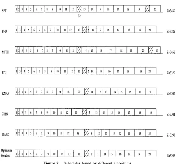
In this section, we illustrate the heuristic algorithms with a numerical example involving 20 jobs. The problem data are as follows, TC ⫽ 182, TL ⫽ 108:

job l 1 2 3 4 5 6 7 8 9 10 11 12 13 14 15 16 17 18 19 20

pl 3 3 6 6 8 9 9 9 10 11 11 13 13 13 13 14 15 16 16 17

We now explain briefly how each algorithm proceeds for this problem.

SPT: The jobs are already arranged in the SPT order. The first 12 jobs fit into the first tool, whereas 2 more tools are needed for the remaining 8 jobs. The resulting schedule, shown in Figure 2, has a total completion time of 3439 units.

FFD: The jobs are now rearranged in the LPT order. The initial FFD schedule has jobs 14 –20 in reverse order followed by job 2 on tool 1 and jobs 3–13 in reverse order followed by job 1 on tool 2. Conformance with the structural properties are now checked. Since the jobs are not SPT ordered on the individual tools (Property 1), they are first reordered as such. We then see that the (ti⫹ TC)/␩iratio for tool 1, (107⫹ 182)/8, is not less than the same ratio for tool 2, (108 ⫹ 182)/12; since this contradicts Property 3, the tool positions are switched. The final schedule with a total completion time of 3329 units is shown in Figure 2.

MFFD: Since the SPT solution uses only 3 tools, we set␮ to 1. Thus, at first, jobs 1–12 are SPT scheduled on tool 1; then jobs 13–20 are FFD scheduled, putting jobs 14 –20 in the LPT order on tool 2 and job 13 on tool 3. The final schedule, upon application of the structural properties, is shown in Figure 2 and is seen to have a total completion time of 3452.

EGI: At stage 1: k ⫽ 1 and pmin ⫽ 3. The EGI rankings obtained are as follows:

q 1 2 3 4 5 6 7 8 9 10

EGIqk 0.00 0.00 ⫺0.47 ⫺0.47 ⫺5.79 ⫺9.94 ⫺9.94 ⫺9.94 ⫺22.10 ⫺29.26

q 11 12 13 14 15 16 17 18 19 20

EGIqk ⫺29.26 ⫺46.57 ⫺46.57 ⫺46.57 ⫺46.57 ⫺73.23 ⫺85.89 ⫺99.55 ⫺99.55 ⫺121.20 Jobs 1 and 2 have the largest EGI value; job 1 is chosen to be scheduled first. We continue in this manner until stage 20 to obtain a complete schedule. The final schedule, upon revision, is shown in Figure 2 and has a total completion time of 3329.

Knap: Since␥ ⫽ 0.7 and 0.7 䡠 TL⫽ 75.6, the first 75 units of any tool’s life will be filled with the available jobs using the SPT rule. Here jobs 1–10 totaling 74 units of processing are first assigned to tool 1. The remaining life RL equals 34 (⫽ 108 ⫺ 74). The knapsack formulation is solved for jobs 11–20 yielding x18 ⫽ x20⫽ 1. Therefore, jobs 18 and 20 are

assigned to tool 1 as well. The process is repeated for tool 2. The final schedule, with a total completion time of 3305, is shown in Figure 2.

2Bin: 2Bin starts with the SPT schedule shown in Figure 2. The first and third blocks are chosen at random in the first iteration. The knapsack formulation is solved for jobs 1–12 and 20; all xqexcept x5are 1. Thus tool 1 gets jobs 1– 4, 6 –12, and 20, and tool 3 gets job 5; tool 2

retains jobs 13–19. At this stage, the new schedule is revised using the structural properties; this results in assigning job 5 first on tool 2 and eliminating tool 3. The schedule obtained is also the final schedule (as shown in Fig. 2) and has a total completion time of 3301.

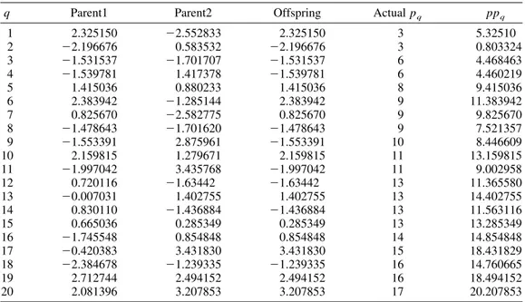
GAPS: We just show one iteration of GAPS using SPT as the base heuristic. An initial population of 50 chromosomes is generated, and the objective function value corresponding to each chromosome is computed. Two parents, Parent1 and Parent2, are now chosen from this population as described earlier. The perturbation vectors for Parent1 and Parent2 are shown in Table 1.

The crossover point is randomly chosen to be 11. The offspring thus copies the first 11 genes from Parent1 and the remaining genes from Parent2. The offspring vector as well as the corresponding perturbed processing times (represented as ppq) are shown in Table 1. At this

stage, mutation is attempted with a probability of 0.1; but it does not occur here. The base heuristic, SPT, is next applied to the perturbed processing times, and it yields the following schedule:

2 4 3 1 8 9 11 5 7 12 6 14 TC 10 15 13 18 16 17 19 TC 20

Upon the use of the actual processing times and the application of the structural properties, we get a schedule with a total completion time of 3446 as shown below:

1 2 3 4 5 6 7 8 9 11 12 14 TC 10 13 15 16 17 18 19 TC 20

The procedure is repeated 1000 times each for both base heuristics SPT and FFD. The final schedule with a total completion time of 3298 is shown in Figure 2.

Optimal Solution: The optimal schedule in this case turns out to be different from all the schedules delivered by the various heuristics. The optimal value of the total completion time, found by the mixed 0 –1 linear program of Section 3, is 3293; the associated schedule is shown in Figure 2.

6. COMPUTATIONAL RESULTS

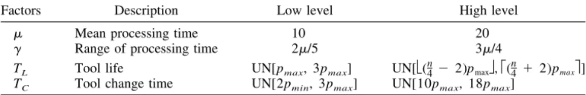
In this section, we report on the performance testing of the proposed algorithms. All the algorithms are coded in the C language and compiled with the Gnu C compiler. The knapsack formulations are solved by using the callable library routines of the CPLEX MIP solver on a Sun-Sparc 1000E. We use a 24full-factorial design involving 4 experimental factors that may affect the performance of the algorithms; the factors and their 2 levels are shown in Table 2. The

Table 1. GAPS example.

q Parent1 Parent2 Offspring Actual pq ppq

1 2.325150 ⫺2.552833 2.325150 3 5.32510 2 ⫺2.196676 0.583532 ⫺2.196676 3 0.803324 3 ⫺1.531537 ⫺1.701707 ⫺1.531537 6 4.468463 4 ⫺1.539781 1.417378 ⫺1.539781 6 4.460219 5 1.415036 0.880233 1.415036 8 9.415036 6 2.383942 ⫺1.285144 2.383942 9 11.383942 7 0.825670 ⫺2.582775 0.825670 9 9.825670 8 ⫺1.478643 ⫺1.701620 ⫺1.478643 9 7.521357 9 ⫺1.553391 2.875961 ⫺1.553391 10 8.446609 10 2.159815 1.279671 2.159815 11 13.159815 11 ⫺1.997042 3.435768 ⫺1.997042 11 9.002958 12 0.720116 ⫺1.63442 ⫺1.63442 13 11.365580 13 ⫺0.007031 1.402755 1.402755 13 14.402755 14 0.830110 ⫺1.436884 ⫺1.436884 13 11.563116 15 0.665036 0.285349 0.285349 13 13.285349 16 ⫺1.745548 0.854848 0.854848 14 14.854848 17 ⫺0.420383 3.431830 3.431830 15 18.431829 18 ⫺2.384678 ⫺1.239335 ⫺1.239335 16 14.760665 19 2.712744 2.494152 2.494152 16 18.494152 20 2.081396 3.207853 3.207853 17 20.207853

processing times are drawn randomly from a discrete uniform distribution over [ pmin, pmax], where pminis ␮ ⫺ range and pmaxis ␮ ⫹ range and ␮ is the mean processing time. We consider 3 different problem sizes (n ⫽ 20, 50, and 100) and 10 problem instances for each combination of the 4 factors and the problem size. Thus, a total of 480 randomly generated problem instances are solved using the proposed algorithms.

The performance measures used in evaluating the experimental results are the total comple-tion time values and the run times in CPU seconds. The relative differences among the solucomple-tions from the various algorithms are calculated in two ways. The first deviation measure, denoted by d1, is the relative percentage deviation of the heuristic solution value from the minimum obtained. It is calculated as: d1⫽ 100(h ⫺ min)/min, where h is the solution value delivered by a given heuristic and min is the minimum of all solution values obtained. The second deviation measure, d2, is the relative deviation of a solution value from the minimum, scaled by the range of all solution values. It is calculated as: d2⫽ (h ⫺ min)/(max ⫺ min), where max is the maximum of all solution values; consequently, the results are normalized between 0 and 1, 0 corresponding to the best solution.

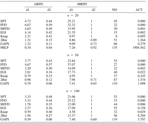
Performance of all seven algorithms are presented using the deviation terms d1 and d2 in Table 3. In this table, ARPD is the average relative percentage deviation, MRPD is the maximum relative percentage deviation, NO is the number of problem instances for which a given heuristic gives the best result, and ACT is the average computation time in CPU seconds. The summary results are presented for the different problem sizes separately. For n⫽ 20, we have also solved the MILP formulation given in Section 3 to find an optimal solution for evaluating the absolute performance of the heuristics. Since some of the problem instances took a long computation time, we had to put a time limit of 3600 s for the CPLEX MIP solver. Therefore, in 25 runs out of 160, the upper bound solutions found by the CPLEX MIP solver at the end of the time limit were worse than the corresponding solutions found by the proposed GAPS algorithm in less than a second. We can see from the results that the computation time requirements are reasonable for all the heuristic algorithms.

The highest total completion time values on the average come from the FFD and SPT algorithms. This is expected since all the other heuristics are developed in order to improve upon these two simple rules. We get better solutions with the EGI and MFFD algorithms, which require almost the same amount of computation time. Moreover, the FFD rule’s inferior performance indicates that minimizing the number of tool switches may not be a satisfactory approach for scheduling purposes. The FFD heuristic may deviate up to 37.07% from the best result; this happens in a problem instance where all the factors are at high levels. Thus, we see that our scheduling problem cannot be viewed as merely a bin-packing problem even when the tool change time is high.

The MFFD heuristic performs better than the first two heuristics. The reason for this is that MFFD’s main advantage comes from assigning more jobs to the first few tools, and it combines the SPT and FFD rules. Overall, among the single pass dispatching heuristics proposed, Knap is the best in terms of the d1 value, whereas EGI for the d2 value. The 2Bin and GAPS heuristics

Table 2. Experimental factors and levels.

Factors Description Low level High level

␮ Mean processing time 10 20

␥ Range of processing time 2␮/5 3␮/4

TL Tool life UN[pmax, 3pmax] UN[( n

4 ⫺ 2)pmax, ( n

4 ⫹ 2)pmax]

give better results than all the others do, GAPS being clearly the best. We also see from the number of best (NO) column that GAPS dominates all the other algorithms, and from its maximum d2 values that GAPS never has performed the worst in these 480 problem instances. We report the effects of the tool life and tool change times on the d1 value in Table 4 (note that a 0 and a 1 in the first column respectively represent the low and the high level of the associated factor). The values shown are averages over 120 randomly generated problem instances. It is observed that, when the tool change time is high, the deviation of SPT from the best increases significantly. When the tool life is low and the tool change time is high, the average relative percentage deviation of SPT is as much as 10.07%. In this case, the perfor-mance of FFD is much better than that of SPT. However, when the tool life is also at a high

Table 3. Summary results.

ARPD MRPD NO ACT d1 d2 d1 d2 n ⫽ 20 SPT 4.72 0.44 25.21 1 45 0.000 FFD 6.67 0.59 32.32 1 22 0.000 MFFD 4.65 0.49 15.95 1 30 0.001 EGI 4.14 0.42 21.35 1 33 0.002 Knap 2.31 0.41 9.97 1 8 0.095 2Bin 1.31 0.15 8.86 0.89 51 1.264 GAPS 1.22 0.11 9.09 0.73 66 0.279 MILP 0.34 0.04 7.26 0.92 135 1904.562 n ⫽ 50 SPT 3.77 0.43 23.84 1 52 0.000 FFD 4.67 0.57 37.07 1 27 0.000 MFFD 3.20 0.50 14.09 1 32 0.003 EGI 2.81 0.34 17.73 1 40 0.022 Knap 0.79 0.33 4.95 1 37 0.245 2Bin 0.96 0.12 7.96 0.71 67 1.534 GAPS 0.70 0.06 7.41 0.65 110 1.098 n ⫽ 100 SPT 3.33 0.48 21.06 1 53 0.000 FFD 3.31 0.44 25.22 1 33 0.000 MFFD 1.78 0.35 12.00 1 44 0.006 EGI 2.37 0.36 17.09 1 55 0.158 Knap 0.59 0.40 4.58 1 32 0.629 2Bin 1.94 0.27 13.37 1 56 8.204 GAPS 0.59 0.06 7.40 0.60 119 3.707

Table 4. Average percentage deviations (d1) for changing TLand TCfactors.

TL, TC SPT FFD MFFD EGI Knap 2Bin GAPS

00 4.22 5.08 3.26 3.94 1.39 1.69 0.81 01 10.07 6.33 5.24 6.63 1.74 3.30 1.97 10 0.18 0.90 0.77 0.17 0.86 0.16 0.10 11 1.29 7.24 3.58 1.68 0.94 0.47 0.48

level, we see that the performance of SPT is not as bad. In this situation, FFD’s deviation increases to 7.24%. This shows again that even when the tool change time is high, the bin-packing solution may not give good results for the scheduling problem.

In summary, we see from the computational results that all the other algorithms provide improvements over the performance of SPT and FFD. Using GAPS, we find schedules that improve the total completion time values over an SPT schedule by up to 3.50% on the average and 16.12% for the maximum and over an FFD schedule by 5.45% on the average and 23.23% for the maximum absolute percent deviation, for relatively small problem sizes. When there are a relatively large number of jobs (say 100), GAPS continues to provide improvements over SPT and FFD in the order of 2.74% on the average and 17.82% for the maximum relative percent deviation. The computation time requirements for all the proposed algorithms are quite low.

7. CONCLUSION

We have introduced a scheduling problem that considers the tool change requirements due to tool wear in flexible manufacturing systems. In manufacturing settings, tool changes are done more often due to tool wear than due to part mix (because of the relatively short lives of the cutting tools). The existing scheduling models ignore the tool replacement constraints and hence could lead to infeasible solutions, whereas the existing tool loading models by assuming infinite tool change times ignore the job attributes and hence could lead to inferior results (as shown by our computational results).

Our focus in this paper has been on the minimization of the total job completion time. In terms of this scheduling problem and its solution, we have proposed a number of heuristics based on dispatch rules and local search, and have tested the absolute/relative performance of the various algorithms. It has been seen that the other algorithms proposed generally outperform the better-known SPT and FFD dispatch rules.

Before we conclude, a few remarks may be in order concerning future research directions. Clearly, one can study the same model as ours in the presence of different scheduling criteria such as the weighted completion time and the weighted tardiness. (It should be noted that much of what we have done here extend rather easily to the weighted completion time case.) In addition, one can relax the assumption of a single tool type and allow multiple tool types and different tooling requirements for the jobs. Finally, we have assumed in this study that the tool life and the processing times are constant and given. However, processing times can be controlled by changing the machining conditions such as cutting speed and feed rate, which directly affect tool wear. This possibility can be incorporated into the model and an objective such as the minimization of manufacturing and scheduling related costs can be pursued.

REFERENCES

[1] I. Adiri, J. Bruno, E. Frostig, and A.H.G. Rinnooy Kan, Single machine flow-time scheduling with a single breakdown, Acta Inf 26 (1989), 679 – 696.

[2] M.S. Akturk and S. Avci, Tool allocation and machining conditions optimization for CNC machines, Eur J Oper Res 94 (1996), 335–348.

[3] M.S. Akturk, J.B. Ghosh, and E.D. Gunes, Scheduling with tool changes to minimize total completion time, Technical Report 99-05, Department of Industrial Engineering, Bilkent University, Ankara, Turkey, 1999.

[4] S. Anily, J. Bramel, and D. Simchi-Levi, Worst-case analysis of heuristics for the bin-packing problem with general cost structures, Oper Res 42 (1994), 287–298.

[5] Y. Crama, Combinatorial optimization models for production scheduling in automated manufacturing systems, Eur J Oper Res 99 (1997), 136 –153.

[6] S.W. Flanders and W.J. Davis, Scheduling a flexible manufacturing system with tooling constraints: An actual case study, Interfaces 25 (1995), 42–54.

[7] E. Gray, A. Seidmann, and K.E. Stecke, A synthesis of decision models for tool management in automated manufacturing, Manage Sci 39 (1993), 549 –567.

[8] D.S. Johnson, A. Demers, J.D. Ullman, M.R. Garey, and R.L. Graham, Worst-case performance bounds for simple one-dimensional packing algorithms, SIAM J Comput 3 (1974), 299 –325. [9] P. Kouvelis, An optimal tool selection procedure for the initial design phase of a flexible

manufac-turing system, Eur J Oper Res 55 (1991), 201–210.

[10] C.Y. Lee and S.D. Liman, Single machine flow-time scheduling with scheduled maintenance, Acta Inf 29 (1992), 375–382.

[11] C.Y. Lee and S.D. Liman, Capacitated two-parallel machines scheduling to minimize sum of job completion times, Discrete Appl Math 41 (1993), 211–222.

[12] C.Y. Lee, Minimizing the makespan in two-machine flowshop scheduling problem with an avail-ability constraint, Oper Res Lett 20 (1997), 129 –139.

[13] C.Y. Lee, Machine scheduling with an availability constraint, J Global Optim 9 (1996), 395– 416. [14] X. Qi, T. Chen, and F. Tu, Scheduling the maintenance on a single machine, J Oper Res Soc 50

(1999), 1071–1078.

[15] K.E. Stecke, Formulation and solution of nonlinear integer production planning problems for flexible manufacturing systems, Manage Sci 29 (1983), 273–288.

[16] R.H. Storer, D.S. Wu, and R. Vaccari, New search spaces for sequencing problems with application to job shop scheduling, Manage Sci 38 (1992), 1495–1509.

[17] C.S. Tang and E.V. Denardo, Models arising from a flexible manufacturing machine, Part I: Minimization of the number of tool switches, Oper Res 36 (1988), 767–777.

[18] C.S. Tang and E.V. Denardo, Models arising from a flexible manufacturing machine, Part II: Minimization of the number of switching instants, Oper Res 36 (1988), 778 –784.

[19] P. Tomek, Tooling strategies related to FMS management, FMS Mag 5 (1986), 102–107.

[20] D. Veeramani, D.M. Upton, and M.M. Barash, Cutting tool management in computer integrated manufacturing, Int J Flexible Manuf Syst 4 (1992), 237–265.