Free-form solid modeling using deformations

FREE-FORM SOLID MODELING USING

DEFORMATIONS

By

Uğur Güdükbay

June 1989

I certify that I have read this thesis and that in my opinion it is fully adequate, in scoi^e and in quality, as a thesis for the degree of Master of Science.

r

Prof. Dr. Bülent ÖZGÜÇ (Princijaal Advisor)

I certify that I have read this thesis and that in my opinion it is fully adequate, in scope and in quality, as a thesis for the degree of Master of Science.

J h c-t

Prof. Dr. M ehm et_^ray

I certify th at I have read this thesis and that in my opinion it is fully adequate, in scope and in quality, as a thesis for the degree of Master of Science.

Asst. Prof. Dr. Varol Akman

Approved for the Institute of Engineering and Sciences:

'A _{iC > a}

ABSTRACT

FREE-FORM SOLID MODELING USING DEFORMATIONS

Uğur Güdükbay

M.S. in Computer Engineering and

Information Sciences

Supervisor: Prof. Dr. Bülent ÖZGÜÇ

June 1989

One of the most important problems of available solid modeling systems is that the range of shapes generated is limited. It is not easy to model ob­ jects with free-form surfaces in a conventional solid modeling system. Such objects can be defined arl^itrarily but then operations on them are not trans­ parent and complications occur. A method for achieving free-form effect is to define regular objects or surfaces, then deform them. This keeps various properties of the model intact while achieving the required visuaJ appear­ ance. This thesis explains a number of geometric modeling techniques with deformations applied to them in attempts to combine various approaches de­ veloped so far. Regular deformations, which include twisting, bending, and tapering, and free-form deformation technique are combined as a new defor­ mation method. This eliminates some of the disadvantages peculiar to each method and utilizes the advantages of both.

Keywords: Deformations, geometric modeling of solids, free-form surfaces, user interface design, shading, hidden surface elimination, computer graphics.

ÖZET

DEFORMASYON TEKNİKLERİ KULLANILARAK

DÜZENSİZ NESNELERİN MODELLENMESİ

Uğur Güdükbay

Bilgisayar Mühendisliği ve Enformatik Bilimleri Yüksek Lisans

Tez Yöneticisi: Prof. Dr. Bülent ÖZGÜÇ

Haziran 1989

Bugüne kadar yapılmış olan katı modelleme sistemlerinin en önemli sorun­ larından birisi de üretilebilen şekillerin kısıtlı olmasıdır. Alışılagelmiş bir katı modelleme sisteminde düzensiz jdizeyleri olan nesnelerin modellenmesi kolay değildir. Bö}de nesneler, üzerindeki her nokta verilerek tanımlanabilir, fakat bu yöntem kullanıldığında bu nesneler üzerindeki işlemler belirgin olmamakta ve bazı zorlukizır ortaya çıkmaktadır. Bu nesnelerin modellenmesinde etkili bir yöntem de düzenli şekilleri oluşturduktan sonra onlar üzerinde defor- masyon tekniklerini uygulamaktır. Bu yolla gerekli nesneler elde edilirken ortaya çıkan zorluklar da önlenmekte ve işlemlerde açıklık sağlanmaktadır. Bu araştırm a bazı modelleme yöntemlerine deformasyon tekniklerinin uygu­ lanması ve deformasyon tekniklerinde bugüne kadar kullanılan değişik j'^akla- şımlarm birleştirilmesi konuları ile ilgilidir. Kıvırma, bükme ve inceltme gibi düzenli deformasyonlar serbest deformasyon tekniği ile birleştirilerek yeni bir deformasyon yöntemi elde edilmiştir. Böylece bu yöntemlere özgü bazı kısıtlamalar yokedilmiş ve her iki yöntemin yeteneklerinden daha etkin bir şekilde yararlanılmıştır.

Anahtar Kelimeler: Deformasyon, katiların geometrik modellenmesi, dü­ zensiz nesneler, kullanıcı arabirimleri, tarama, görünmeyen yüzeyleri j’oketme, bilgisayar grafiği.

ACKNOWLEDGMENTS

I would like to thank my thesis advisor, Prof. Biilent Özgüç, for his guidance and support during the development of this study.

I appreciate mj^ colleagues, Aj'dm Açıkgöz, Veysi İşler, Aydın Kaya, Ah­ met Coşar, Faruk Polat, İsmail Hakkı Toroslu, Cem Evrendilek, and Ufuk Çelikkan, for their valuable discussions and comments.

I am also grateful to Cemil Türün for his technical help.

Special thanks to Prof. Mehmet Baray and Asst. Prof. Varol Akman for their encouragement and support.

TABLE OF CONTENTS

1 INTRODUCTION 1

2 MODELING 4

2.1 History of M o d e lin g ... 4

2.1.1 Classification and Properties of Solid Modelers . . . . 6

2.1.2 Modeling Free-Form S u rfa c e s ... 7

2.2 Modeling in Our S y stem ... 8

2.2.1 Supercpiadrics... 8 2.2.2 Bezier S u rfa c e s... 13 3 DEFORMATIONS 18 3.1 Regular D e fo rm a tio n s... 19 3.1.1 Scaling ... 20 3.1.2 Tapering ... 21 3.1.3 T w isting... 21 3.1.4 B e n d in g ... 24 3.2 Free-Form Deformations ( F F D ) ... 25 3.2.1 Formulation of FFD’s ... 27 vi

3.3 Combination of Regular Deformations and FFD Technique . 30 3.4 An Example of Generating a Composite S h a p e ... 32

4 DISPLAY FACILITIES PROVIDED BY THE SYSTEM 36

4.1 Hidden Surface E lim in a tio n ... 36

4.2 S h a d in g ... 38

5 THE USER INTERFACE 42

5.1 Facilities for Creating Bezier Surfaces and Superquadrics . . . 42

5.2 Facilities for Deforming O b je cts... 43

6 CONCLUSIONS 45

REFERENCES 46

APPENDICES 49

A THE USER’S MANUAL 49

A .l Description of the Panel Items ... 49

A.2 Help Facilities Provided by the S ystem ... 51

LIST OF FIGURES

2.1 Superquadric ellipsoids with different exponents... 11

2.2 Superquadric hjqDerboloids of one piece with different exponents. 12 2.3 Superquadric hyperboloids of two pieces with different expo­ nents... 14

2.4 Superquadric toroids with different exponents... 15

2.5 Four Bezier surfaces... 17

3.1 Tapered superquadric ellipsoids... 22

3.2 Twisted superquadric ellipsoids... 23

3.3 Bent superquadric ellipsoids... 26

3.4 A twisted, tapered superquadric ellipsoid, and a tapered, bent superquadric ellipsoid... 26

3.5 An ellipsoid deformed using different FFDs... 29

3.6 Results of applying combination of regular deformations and FFDs... 31

3.7 The rounded bar initially... 33

3.8 The rounded bar after applying FFD three times... 33

3.9 Telephone handset generated... 34

3.10 Telephone handset (hidden surfaces eliminated). 34 3.11 Telephone handset (shading applied)... 35

4.1 Shaded Bezier surfaces... 39

4.2 Shaded superquadric objects... 40

4.3 Objects obtained through deformations with shading applied. 41

5.1 The layout of the screen while parameters of superquadrics are given... 43

5.2 A lattice of control points created and deformed by our sj'^stem. 44

A.l The help window giving a general idea about the system. . . 52

A.2 The help window explaining how scaling factors of superquadrics are entered... 52

A.3 The help window explaining the entry of control points of Bezier Surfaces... 53 A.4 The help window giving a general idea for the operations that

can be done by the system... 53

A.5 The help window explaining how parameters are entered for the bending operation... 54

A.6 The help window explaining how different twisting and taper­ ing functions can be entered for these operations... 54

A.7 The help Avindow explaining how rotation parameters are en­ tered... 55 A.8 The help window explaining how scaling parameters are entered. 55

A.9 The help window explaining how the lattice of control points are created and modified for performing an FFD ... 5G

A. 10 The help window explaining how translation parameters are entered... 56

1. INTRODUCTION

A system for deforming three dimensional models to obtain objects with free­ form surfaces is explained in this thesis. The system is implemented using C language [15] on a Unix ^ workstation environment. In the implementation of the system, care has been taken to include user interface facilities to simplify the usage [14].

In advanced CAD/CAM applications, designers need to model solid ob­ jects with complex surfaces [16]. Objects whose surfaces are free-form defy

description in terms of analytical surfaces such as planes, cones, spheres, or toroids [8]. There are various approaches to model objects with free-form surfaces in a solid modeling system.

One approach uses Boolean operations on arbitrary free-form surfaces. To implement Boolean operations, the computation of intersecting curves between two different free-form surfaces is required. This takes a long com­ putation time since intersection algorithms compute points iteratively and perform some type of curve fitting that yields an approximate intersection curve. Because of this, the interpolating curve will never lie exactly on both surfaces. Consequently, intersection algorithms are unreliable.

The second approadi involves generating free-form surfaces from a poly­ hedron. This approacli uses rounding operations on polyhedral objects for integrating solid modeling and free-form surface modeling [9]. Since complex calculations are not needed, computation time and reliability are not prob­ lems. However, there are several restrictions in the range of shapes generated.

Another approach to model free-form surfaces is based on parametric polynomial functions [10]. This is a unified approach and geometric opera­ tions can be performed with equal facility on simple primitives and complex

sculptured geometries by using it. This approacli combines a number of para­ metric polynomial geometry representations, such as Bezier, Coons, B-spline into a unified modeling system that is capable of interchanging between these representations through mathematical transformations.

A new approaclr, deformations, is similar to the second approach in the sense that both provide methods of changing the existing models to create irregular classes of objects. Deformations, first introduced by Alan Barr [4], are highly intuitive and easily visualized set of operations. Deformations al­ low the user to treat a solid as if it were constructed from a special type of topological putty or clay, which may be bent, twisted, tapered, compressed, expanded and otherwise transformed into a final shape. Deformations can be incorporated into traditional CAD/CAM solid modeling and surface patch methods, reducing the data storage requirements for simulating flexible ge­ ometric objects, such as objects made of metal, fabric or rubber. Without deformations, to simulate an irregular object, one has to save every point on the object. However, one can create a regular object and then apply deformations to it to create an irregular object with much less data.

Our system currently uses superquadric objects and Bézier surfaces to model regular classes of objects. There are two main approaches used to deform solid geometric moclels:

• Regular deformations [4].

• Free-form deformation (FFD) technique [21].

Our system combines these two approaches for deforming regular classes of objects to create objects with free-form surfaces. Both deformation tech­ niques can be applied hierarchically and interchangeably in our system. The combination seeks to offer benefits of both regular deformations and FFD technique.

The remaining parts of this thesis are organized as follows. Chapter 2 surveys the concepts related to geometric modeling by explaining the history of geometric modeling and shows how objects are modeled in our implemen­ tation. Mathematical details of superquadrics and Bezier surfaces are also explained in this part.

Chapter 3 describes different deformation techniques and compares them by giving the advantages and disadrantages of them. It also gives the rea­ sons why these techniques are com]:>ined to obtain a different deformation

technique and explains how deformations are implemented in our system by giving examples.

Chapter 4 gives a detailed explanation about the display facilities provided by the system (shading and hidden surface elimination) and describes the methods used for these purposes together with the reasons why they are used.

Chapter 5 contains information about the user interface issues of the im­ plementation. The user interface facilities for creating the objects that the user desires and manipulating them through the set of operations provided by the system are exidained in detail.

2. MODELING

2.1 H istory o f M od elin g

The application of computers to drafting and design started with Sketchpad, which is a remarkable program devised by Ivan Sutherland at MIT in the earl}'^ 60’s. First, the techniques of Sketchpad were applied to circuit design where the connectivity or topological properties of the data, represented as a graph of nodes and links, are important [6].

Later, drafting systems progressed in two ways; firstly, in the amount of structure captured and in the variety of graphics entities represented, and secondly, by moving from two to three dimensions. Wireframe models have emerged as a result of these developments where perspective views and re­ moval of hidden lines have gained importance.

Wireframe models can be defined as a collection of curve segments which represents an object’s edges. Wireframe models have some serious deficien­ cies. These deficiencies can be listed as follows [19]:

• The wireframe may be ambiguous; it may represent more than one object.

• Nonsense objects such as ii wireframe with one of the edges missing cannot be detected by the system.

• Representation of lines to depict viewpoint-dependent artifacts in the wireframe creates problems.

The first two deficiencies limit various automatic processes that can be done by a system using wireframe modeling. For example, calculating vol­ umes of objects represented by a wireframe and automatic sectioning of them are almost impossible to implement automatically.

A further step in the progress of drafting systems was to allow 3-D wire­ frame models to be surfaced. The surfaces are represented by embedding of the graph formed by edges and vertices of a wireframe model. This embedded graph represents the boundary model of the solid.

The systems addressing the problem of designing classes of parts comes after drafting systems. These systems are dedicated to a family of special products, such as j^umps. They calculate design properties of pumps, gen­ erate pictures of them, etc. These sj'stems cover three stages of product definition, namely, design, analysis, and manufacture. Consequently, they reduce the chance of error from stage to stage. Their drawback is that they are expensive to write and develop, and they can act as a barrier to progress since they embody certain design rules which new knowledge maj' make ob­ solete.

Later, solid modelers have emerged as a new development in drafting systems. The term solid modeling encompasses a body of theory, techniques, and systems focused on informationally complete representation of solids — representations that permit (at least in principle) any well-defined geometric property of any represented solid to be calculated automatically [19].

Solid modeling is a powerful and promising concept for computerized product definition [16]. Systems used in the design of products cover not only design but also analysis and manufacture. This means that the same data are repeatedly used at design, analysis and manufacturing steps. For this reason, if the information were captured in a. suitable, general form at the design time, it could be used again for analysis and for manufacture. In this way, mistakes could be avoided, and time and money saved. This re­ quires to decide on a product representation that is suitable for all types of computations. The representation must be accurate, must contain enough information for all subsequent inquiries to be made, and should be concise. To achieve this goal, solid modelers have been developed.

2.1.1

C lassification and P ro p erties o f Solid M odelers

Solid modelers can be classified into two broad categories: regional (descrip-

tive) modelers, and boundary modelers. Regional modelers can be further

classified as subdivisional modelers and cellular modelers.

One type of descriptive modeler is based on Constructive Solid Geometry (CSG). It uses trees (CSG trees) of building block primitives, such as par­ allelepipeds, spheres, cylinders, etc. combined by geometi'ic transformations and Boolean set operations as a representation of three-dimensional solid objects [20].

Another type of descriptive modeler represents solid objects using half spaces, each described by an equation of the form /(x , y, z) > 0. Some of the CSG models also decompose primitive solids into subtrees whose leaves are halfspaces so that they combine both pure CSG and halfspaces [20].

Modelers using octree methods are in the group of cellular modelers. They represent solid objects by a'binary tree defining recursive subdivision of space and recording which parts are empty and which parts are solid. The trees used to represent two dimensional objects are called octrees and the ones used to represent solid objects are called quadtrees [7].

Subdivisional modelers are similar to cellular modelers, but the subdivi­ sion of space into smaller parts is not necessarily regular, as in the case of cellular modelers.

Boundary (or surface-based) representation techniques describe solid vol­ umes in terms of their enclosing surfaces. Such models can be called solid models when they completely describe the form and the extent of the indi­ vidual surfaces of the objects. They must also contain enough information to determine how the surfaces are joined together to form completely closed and connected volumes [11].

Boundary representation (B-rep) techniques use some low-level operators, called Euler operators, as a convenient and consistent way of creating and modifying the topological data of the solid model. Most common Euler op­ erators are [6]:

1. Create shell (a shell of an object S is defined as a maximal connected set of faces of 5 ), face (face's can be defined as contiguous surface areas of the volume enclosed by face boundaries), and vertex.

2. Add edge and vertex.

3. Add edge, face and loop (a loop on a face / is defined as a closed chain of edges bounding / ) .

4. Add genus and loop, remove face and loop. 5. Add loop, remove shell, face and loop.

Boolean operations are not included in the representation of a B-rep model, but they often are employed as one of the means of creating and manipulating the model. Since B-rep systems require an explicit representa­ tion of the boundary of the solid, they must evaluate the new boundary that is the result of the Boolean operation applied [8].

Other methods for creating and manipulating geometry in B-rep sj'^stems include sweeping, whicli defines the bounding surfaces of the solid by moving a cross-section along a path in space, and tweaking, which performs local operations on the geometry,'but leaves the topology of the model unchanged. Tapering is an example to tweaking. Some other operations which introduce strain, shear, and torsion into models are bending, which changes the topology of a model in a well-defined way, blending, which rounds off and chamfer sharp edges, and stretching, which occurs in physical bending.

2.1.2

M odeling Free-Form Surfaces

Although there are a number of solid modeling systems that can be used as a basis for product modeling, solid modeling capabilities have not been fully utilized. There are several technical problems remaining, such as dimension­ ing and tolerancing, user interface, and speed and reliability of processing [16]. Treatment of solid objects with free-form surfaces is another major problem of curi'ent solid modeling systems. Objects with free-form surfaces cannot be described in terms of analytical functions. Some examples of objects with free-form surfaces are the fender of a sports car, the transition between the wing and fuselage of an aircraft, the hull of a destroyer, the handle of a hand­ held mixer, etc. [8]. Free-form surface design capability should be integrated into solid modeling systems in order to model objects with complex surfaces. The approaclies for free-form surface design (explained in Chapter 1) can be used in solid modeling systems for this purpose.

2.2 M od elin g in Our S ystem

Since our system uses regular objects to create objects with free-form sur­ faces, we have to provide methods to model these regular objects. In the implementation of the system, two different surface modeling methods based on param etric polynomial functions, namely superquadrics and Bezier sur­ faces, are used to model regular classes of objects. They are explained in detail with some examples in the following sections.

2.2.1

Superquadrics

One long-term goal of computer graphics and numerical methods for three- dimensional design is a unified mathematical formalism. Such a unified m ath­ ematical formalism for geometric representation and computation provides a natural base for a geometric modeler of considerable versatility and robust­ ness [10]. Superquadric objects show potential to achieve this goal [3]. Su­ perquadric objects are a new collection of smooth parametric objects produc­ ing a new spectrum of flexible forms. The chief advantage of superquadrics is that they allow complex solids and surfaces to be constructed and altered easily by changing a few interactive parameters. The superquadrics family mainly consists of superquadric ellipsoids, toroids, hyperboloids of one piece, and hyperboloids of two pieces. These shapes differ from the corresponding quadrics in the exponent of their terms. The exponent of their terms, two for the quadric shapes, is replaced by an arbitrary positive number. By changing the exponent of the terms, the shapes can be rounded, pinched, and can have different properties in different sections.

Superquadrics can be defined by either nonparametric or parametric equa­ tions. The parametric form is used for calculation, since surface points and normal vectors can be generated more easily with this method than with the implicit form, but the sampled points are sometimes very unevenly spaced. The nonparametric form, which is developed using computational geometry techniques, uses explicit equations or series approximations for generating points on the curve. Advantages of the nonparametric form are [2]:

• It naturally produces equally spaced points. • It requires much less CPU time for each point. • It can produce surfaces of great generality.

Our implementation uses parametric equations to generate superquadrics since generation of surface points is easier with this method. Also, we need normal vectors for shading and hidden surface elimination. Calculation of normal vectors at each surface point is much easier using parametric equa­ tions. To speed up the generation of points, the values th at will be needed to produce the points are calculated once and they are stored in look-up tables so that they will be retrieved when they are needed.

The mathematics used to define superquadrics can be summarized as follows [3].

Given are two two-dimensional curves

h{u) = hi{Lj)

h2(oj) , Wo < w < Wi,

and

22l(?7) =

777.2(77) ,770 < 77 < 771.

The spherical product x = m ® h oi the two curves is a surface defined as

477, w) = 777.1 ( 7 7 ) /? .i( w ) 777i(77)/l2(w) 777.2(77) ^ ^ ^ »70 <11 <

ih-Geometrically, h{u)) is a horizontal curve vertically modulated by 777(7/); 7771(77) changes the relative scale of h, while 7772(77) raises and lowers it. 77 is a north-south parameter, like latitude, whereas w is an east-west parameter, like longitude. Spherical product surfaces can be rescaled by a separate vector

a = [01, 02, 03]^ where T denotes the transpose.

Types of superquadric shapes and the formulation of them are explained in the following sections.

Superellipsoids

Position vector of surface:

^ - f < »? < f

=

t\ is the squareness parameter in the north-south direction and cj is the

squareness parameter in the east-west direction. Cuboids are produced when both €i and €2 are < 1. Pillow shapes are produced when ci ~ 1 and €2 < 1· Pinched shapes eire produced when either Ci or £2 > 2. Flat-beveled shapes are produced when either ej or £2 = 2.

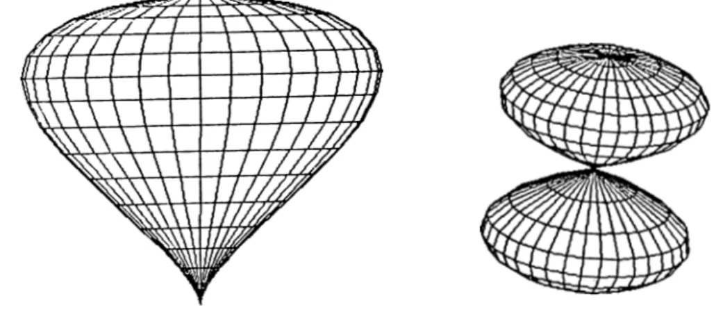
Wireframe examples of superquadric ellipsoids with different exponents are shown in Figure 2.1.

Superhyperboloids of one piece

Position vector of surface:

aised^ TfC^ 02sec'i7/5‘* a^tan^^ rj

-f <7? < f

Wireframe examples of superquadric hyperboloids of one piece with dif­ ferent exponents are shown in Figure 2.2.

Figure 2.2: Supcrquadric hyperboloids of one piece with different exponents.

Superhyperboloids of two pieces

Position vector of surface:

aisec'^'iisec^^u a2sec^^ i]tan^'^io aatan^^ rj

- f <T7< f

02

'

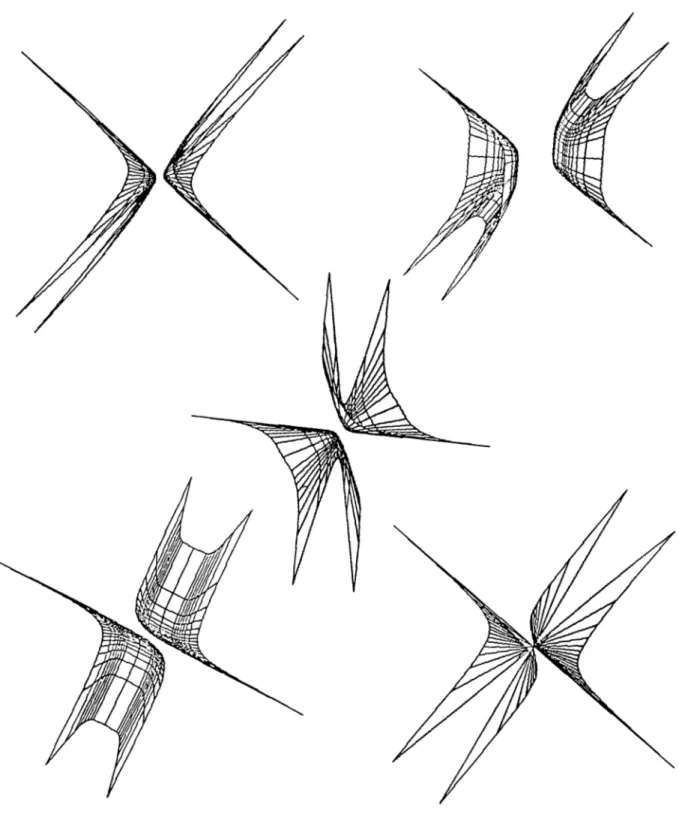
Wireframe exami^les of superquadric hyperboloids of two pieces with dif­ ferent exponents are shown in Figure 2.3.

Supertoroids

Position vector of surface:

£ (t/ ,w) = Oi(a4 + C;>)C:^ 02(^4 + C''* )S ^ — 7T < 77 < 7T — 7T < iO < TT Normal vector: E(li.w) = J_ C2-£i

03*^*)

where 04 = ° ,t, and 2 is the radius of the torus.

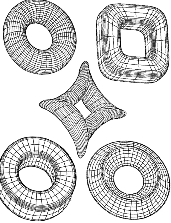
Wireframe examples of superquadric toroids with different exponents are shown in Figure 2.4.

2.2.2

B ezier Surfaces

For an arbitrary curve, it may be difficult to devise a single set of parametric ec^uations that completely defines the shape of the curve. However, any curve can be approximated by different sets of parametric functions over different

Figure 2.3: Superquadric hyperboloids of two pieces with different exponents.

Figure 2.4: Superquaclric toroids with different exponents.

parts of the curve. Since finite degree polynomials are, in many respects, ideal forms for representing and approximating functions, they are used to form these approximations. The smoothness of a curve from one section to another can be described in terms of curve continuity between sections [5].

Parametric equations for surfaces are formulated with two parameters

u and V. A coordinate position on a surface is then represented by the

parametric vector function P (u, u) = (a;(u, u), y(u, v), z(u, u)). The equations for coordinates x, ?/, and ^ are often arranged so that parameters u and v are defined within the range 0 to 1.

To define a curve or surface in design applications, a set of control points indicating the shape of the curve or surface is interactively specified. Bezier formulated a method for displaying curves specified with control points using the Berstein polynomial basis. A useful feature of Berstein basis is its convex- hull property, which means that any curve defined using it smootlily follows the control points without erratic oscillations.

Formulation of Bezier curves can be summarized as follows [5].

Suppose n -|- 1 control points are input and designated as the vectors

Pk — {^kiyki2k)i^ < < n. From these coordinate points, we calculate an approximating Bezier vector function P{u) which represents the three parametric equations for the curve that fits the input control points pk- It can be calculated as

P ( u ) = è p i B i , „ ( u ) (*)

Jt=0

Each Bk,n(u) is a polynomial function defined as 5 , » = C '( n ,A :y ■ ( l- u r - ^ where C{n, k) represents the binomial coefficients

111

C ( n , k ) =

Equation (*) can be written as a set of parametric equations:

x(u) = Y^XkBk,n{u)

k=0

y(.^<) = Y , ykBk,A^i) k=0

•^(^) = ^kBk,n{u)

k=0

Two sets of Bezier curves can be used to represent surfaces of objects specified by input control points. The parametric function for a Bezier surface is formed as the cartesian product of Bezier blending functions:

P{u,v) — ^ Pj,kBj,miu)Bk^ni'v)

j=0 k=0

with pj^k specifying the location of {m + 1) by {n + 1) control points.

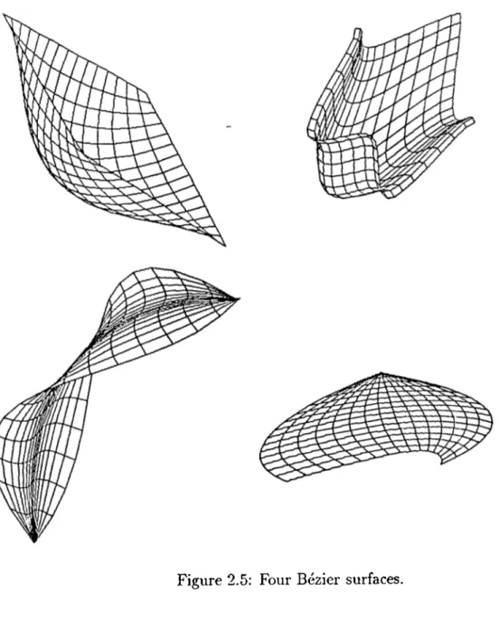
Figure 2.5 shows four Bezier surfaces generated by our system.

Figure 2.5: Four Bezier surfaces.

3. DEFORMATIONS

Since the primary goal of our system is to create the free-form objects and scenes th at the user desires, we have to supply the user with the operations th at can be used to achieve this goal. We have implemented deformations for this purpose. Two deformation techniques are used in the implemen­ tation. Regular deformations [4] simulate twisting, bending, tapering, or similar transformations of geometric objects. Free-form deformation (FFD) technique [21] is mainly developed to define solid geometric model of an ob­ ject bounded by free-form surfaces, and further sculpturing it with flexibility and freedom. Both of these "techniques have advantages and disadvantages.

Although results of FFD can be guessed according to the movement of control points, desired objects can be obtained by trial and error. However, regular defoi'inations are well-defined and their results are straightforward. On the other hand, using FFD as a free-form modeling technique is better than using regular deformations due to the generality of FFD.

A very important disadvantage of FFD is the speed of the deformations since operations on trivariate Berstein polynomials are very costly. It can be made faster by converting trivariate Berstein polynomials to standard power basis polynomials. However, this operation also takes a fair amount of time.

The speed of deforming an object with FFD technique also depends on the number of control points. A deformation defined by larger number of control points can cause the deformed shape to follow the control points more closely than for lower degree deformations [22]. This produces better results at the expense of slowing down the operations. Regular deformations are very fast compared to FFD technique.

These two approaches have some common properties:

• Both approadies can be applied hierarcliically to create complex objects

from simpler ones.

• Both approaches can be applied to any solid modeling scheme.

• Both approaches compute the new x, y, z coordinates of a point as polynomial functions of the original x, y, z coordinates of that point.

Due to the reasons stated above, our system combines the two approaches to alleviate the problems of them and to offer the benefits to the user. When regular deformations are suitable for modeling an object, the user may use them to gain in speed. When they are not sufficient for modeling an ob­ ject, either FFD technique can be used or both of the techniques can be applied hierarclrically and interchangeably. The two deformation techniques are explained in detail with some examples in the following sections.

3.1

R egular D eform ation s

A globally specified deformation of a three dimensional solid is a m athem at­ ical function F which explicitly modifies the global coordinates of points in space. Mathematically, it can be represented by the equation X = F(x) where x represents the point in the undeformed solid, and X represents the points in the deformed solid.

A locally specified deformation modifies the tangent space of the solid. It is used to manipulate the tangent vectors which is used for delineating and constructing the local geometry. In other words, it is used to obtain more general shapes.

Tangent and normal vectors on the undeformed surface may be trans­ formed into the tangent and normal vectors on the deformed surface; the algebraic manipulations for the transformation rules involve a single multi­ plication by the Jacobian matrix ¿ of the transformation function F.

The Jacobian matrix ¿ for the transformation function X = F(x) is a function of X , and is calculated by taking the partial derivatives of F with

respect to the coordinates x i, X2,X3’.

U n ) = _dxi

In other words, the column of X is obtained by taking the partial deri\'ative of F(;c) with respect to .r,.

New tangent vectors of the deformed surface are calculated by multiplying the tangent vectors of the undeformed surface by the Jacobian and new normal vectors of the deformed surface are calculated by multiplying the normal vectors of the undeformed surface by the inverse transpose of the Jacobian matrix.

Each of the regular deformations are explained in detail in the following sections.

3.1.1

Scaling

One of the simplest deformations is a change in the length of the three global components parallel to the coordinate axes. This produces an orthogonal scaling operation which is represented by the following equations:

X = a^x

y = a^y

Z - azz

The components of the Jacobian matrix are given by

■’ '> dxi

’

0 ^

0

0 02

The volume change of a region scaled by this transformation is obtained from the Jacobian determinant, which is 010203. The normal transformation matrix is given by:

det =

02O3 0 0 ^ 0 0103 0 0 0 01O2 /

After converting a point [a;i, 3-2, 3:3]^ lying on a roughly spherical surface cen­ tered at the origin, with normal vector [/Jd ^^2? >^3]^» transformed surface point on the resulting ellipsoidal shape is [oi.Ti, 023'2, 03.T3]^ and the trans­

formed normal vector is parallel to volume ratio between the shapes is 01O2O3.

i

Tapering is making an object become gradually narrower towards one end of it. Mathematically, it differentially changes the length of the two global components without changing the length of the third.

To do a tapering operation along the z-axis, one should choose a tapering function depending on the z-coordinates of the points. When the tapering function f{ z) = 1, the portion of the deformed object is unchanged; the object increases in size as a function of z when f'( z) > 0 and decreases in size when f'{z) < 0. The object passes through a singuleirity at f ( z ) = 0 and becomes everted when f ( z ) < 0. Global tapering along the z-axis is given bj'^ the following equations:

r = f ( z )

X = rx Y = rxj Z = z

Tangent vector transformation matrix is given by

3.1.2

Tapering

1 =

^ r 0 f'{z)x ^ 0 r f'{z)y

0 0 1

Normal vector transformation matrix is given by

=

Examples of tapering are shown in Figure 3.1 where a superellipse is tapered using different tapering functions. The first object is obtained using the tapering function f {z) = and the second one is obtained using

f {z ) = c o s { z ^ ) .

3.1.3

T w isting

A twist operation can be approximated as a differential rotation, just as tapering is a differential scaling of the global basis vectors, ^^^e rotate one

Figure 3.1: Tapered superquadric ellipsoids.

pair of globed basis vectors as a function of height, without altering the third globed basis vector. An exami^le to twisting operation is the twisting of a deck of cards, by which, each card is rotated somewhat more than the card beneath it. Twisting operation preserves the volume of the original solid.

To do a twisting operation along the z-axis, twisting angle 0 should be a function of the z-coordinate of the point to be deformed. Global twisting along the z-axis is given by the following equations:

e

The twist proceeds along the axis at a rate of /'(2 ) radians per unit length in the z direction.

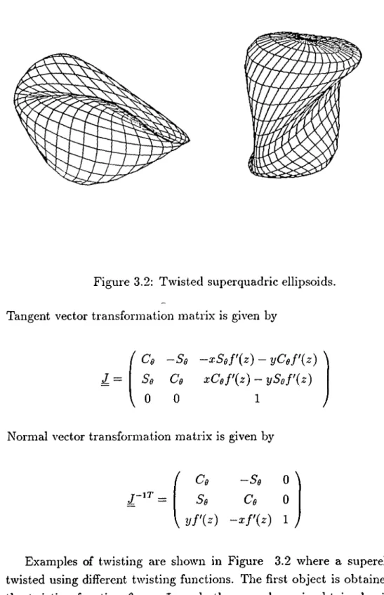
Figure 3.2: Twisted superquadric ellipsoids.

Tangent vector transformation matrix is given by

1 =

Ce - S e - x S o f'iz ) - yC ef'{z) \ Se Ce xC gfXz) - yS o f'(z)

0 0 1

Normal vector transformation matrix is given by

Ce Se y f'( - ) - S e 0 \ Ce 0 - x f i z ) 1

Examples of twisting are shown in Figure 3.2 where a superellipse is

twisted using different twisting functions. The first object is obtained using the twisting function ^ flie second one is obtained using 9 =

Bending simulates an important manufacturing process for fabricating ob­ jects. An example to this operation is the bending of a bar stock or sheet metal.

To make a bending along the y-axis, one has to specify a bent region along the y-axis. The range of the bending deformation is controlled by

y-mini and Углах» with the bent region corresponding to values of у such that Утш < у ^ Утах- The axis of the bend is located along [5,уо, where s is the param eter of the line. The center of the bend occurs at у = уо- The radius of curvature of the bend is p The bending angle $ is constant outside the bent region, changes linearly in the central region. In the bent region, bending rate k, measured in radians per unit length, is constant. Outside the bent region, the deformation consists of a rigid body rotation and translation. The length of the centerline passing through the object along the y-axis does not change during the bending process.

The bending angle в is given by:

в = h{y - Уо) C$ = со${в) Se = sin{9) where yminj У — У min У ^ У? У min ^ У ^ Угпаг ^ Утах^ У ^ Утах

The formula for bending along the у axis centerline is given by the following equations:

.Y = X

Sq{^Z jt) "h Уо? Утт ^ У ^ Утах

^ ^ So{^ it) Уо "I" Утт)? У ^ УтЫ

-S e { z - ¿) + Уо + Ce(y - Утах), У > Утах Cq(^Z ¿) "b ^? Утт ^ У ^ Утах

Z = I Co{z “ i) + ^ + Se(y - ymin), У < Утт Co{z it) it ^^{y Утах), У ^ Утах

3.1.4

B en d in g

Tangent vector transformation matrix is given by 1 = ( 1 0 o ' ' 0 C g ( l - k z ) - S e ^ 0 — kz) C$ y where k = k , y = y

0,

-Normal vector transformation matrix is given by

(1 - =

i 1 - k z 0 0 ^ 0 C$ —Se{l — kz)

y 0 S$ Ce(l — kz) j

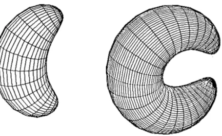
Examples to bending operation are shown in Figure 3.3. In these exam­ ples, bent region includes the whole object. In the first figure, an ellipse is bent 90°, and in the second one an ellipse is bent 360°.

The transformations explained above can be combined with rotation around some axes so that these operations can be performed around other axes than the ones explained above.

Results obtained by applying regular deformations hierarchically are shown in Figure 3.4.

3.2

Free-Form D eform ation s (F F D )

Free-form deformations can be thought of as a method for sculpturing solid models in a free-form manner. FFD can sculpt solids bounded bj»^ any analyt­ ical surface; planes, cjuadrics, parametric surface patches, or implicit surfaces. Its application is not restricted to solid models, but it can also sculpt surfaces or polygonal data.

In our system, two kinds of parametric surface patches, namely Bezier surfaces and superquadrics, are deformed in a free-form manner using FFD techniques. In fact, the objects are apiDroximated using small polygons. Thus, the deformed data are actually polygonal data.

Figure 3.3r Bent superquadric ellipsoids.

Figure 3.4: A twisted, tapered superquadric ellipsoid, and a tapered, bent superquadric ellipsoid.

3.2.1

Form ulation o f F F D ’s

The free-form deformation is initiated by defining a three dimensional grid of control points about the region to be deformed. The objects to be deformed are embedded in the grid of control points that can be interactively deformed as if it is made out of a flexible material. The objects themselves can also be regarded as if they are made out of a flexible material, so th at when the whole grid is deformed, the objects inside them are also deformed respectively.

The control points form a regular lattice which is defined within a paral­ lelepiped generated by three non-coplanar vectors S, T , and U, and a point Xo- Any point has ( s ,t,u ) coordinates in this system such that

X = X q 4" áS -f- t T -|- u U .

In our system, X will tyi^ically be a polygon vertex expressed in (a:, y, z) coordinates, and S ,T , and U are analogous to the unit vectors in X ,Y , and Z direction. The ( s ,i,u ) coordinates of X can be found as follows:

s = T X U · ( X - X o ) T x U - S t = S X U - ( X - X o ) S X U - T u = S X T - ( X - X o ) S x T - U

In our system, the above calculation is not necessary since x, y, and 2 coordinates of the points are calculated automatically. It can be used when the coordinates of a point are given in vector form.

For any point interior to the parallelepiped, 0 < 5 < 1 , 0 < < < 1 , and 0 < u < 1. The grid of control points P,jjt imposed on the jDarallelepiped forms / 4 - 1 planes in the S direction, ?n 4- 1 planes in the T direction, and -f- 1 planes in the U direction. So the number of control points is (/ 4- l)(m 4- l)(i^ 4-1) and their undisplaced locations are defined as

Po-, = Xo4 - 7 S 4 - ^ T + - U

/ m n

The deformation function is defined by a trivariate tensor product Berstein polynomial. The deformation is specified by moving the Pijk from their undisplaced, latticial positions. A point X is transformed to its free­ form deformation position by first computing its (s, t, u) coordinates of X and then evaluating the Berstein polynomial

(1

- .)

m

X

I E (

i=0 V

( 1 - u r - V 'P . y * ] ]

The control points Pijk are actually the coefficients of the Berstein poly­ nomial. For a polygonal model, each node is ¡massed through the deformation function, and the connectivity is unchanged.

Since it is very time consuming to evaluate a tiivariate Berstein poly­ nomial for lots of polygon vertices th at are to be transformed, it is wise to convert the Berstein polynomial to standard power polynomial basis which can then be evaluated using Horner’s method.

Our system uses the algorithms in [22] to convert a Berstein basis poly­ nomial to a standard basis polynomial and to evaluate the power basis poly­ nomial.

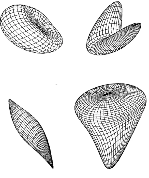
Examples to FFD techniciue are shown in Figure 3.5 where an ellipsoid is deformed using different FFDs.

Figure 3.5; An ellipsoid deformed using different FFDs.

3.3

C om bin ation o f R egular D eform ation s and FFD

Technique

Since FFD is a method for deforming three-dimensional objects in a free-form manner, regular deformations can also be performed using it. However, using FFD to make twisting, bending, and tapering operations brings some unde­ sired effects. For example, when an object is bent using FFD technique, the result will not be as predictable as when the same object is bent using regular deformations. This is also true for other regular deformations. Another rea­ son why using FFD to deform an object is more difficult than using regular deformations is that the user should perform trial and error until the desired object is obtained. FFD technique is slower since using it involves operations with trivariate tensor product Berstein polynomials. Regular deformations are faster since the whole operation is just a single matrix multiplication. Consequently, when regular deformations can perform the desired operation, it is better to use them.

In addition to twisting,-tapering, and bending, Barr [4] explains some operations for deforming objects locally when the Jacobian of the deformation function is known. This is another way of obtaining more general shapes. However, the implementation of local deformations is very difficult. FFD technique Ccin be used to achieve the results that can be obtained by using the local operations described by Barr, since it can either be applied locally or globally.

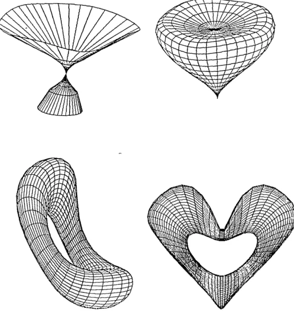
We have applied the two deformation techniques hierarchically to regular classes of objects in our system. Results are shown in Figure 3.6. The first object is obtained by initially tapering a superquadric hyperboloid of one piece and then appljdng an FFD to the tapered object. The second object is also obtained in the same way , but the initial object is an ellipse. The third object is obtained by applying an FFD to a superquadric toroid to compress it and bending the compressed object, and the last object is obtained by tapering a superquadric toroid and applying FFD to the tapered object.

Figure 3.6: Results of applying combination of regular deformations and FFDs.

3.4

A n E xam ple o f G en eratin g a C o m p o site Shape

In this section, the use of the system is described by an example. In the following example, the system is used to generate a telephone handset from a rounded bar. Steps of the process are as follows :

1. First, it is necessary to generate a rounded bar. This is accomplished by creating a superquadric ellipsoid similar to a rectangular prism. The superquadric ellipsoid in Figure 3.7 is generated by setting the “Resolu­ tion” to 72, and giving ei and C2 as 0.52 and 0.52 respectively. Scaling factors are arranged interactively by the user as described in Figure A.2. The superquadric ellipsoid is seen from the top when it is gen­ erated. To obtain the shape in the figure, the initial shape is rotated around X axis.

2. FFD technique is hierarchically applied to the rounded bar to obtain the shape in Figure 3.8. The shape is obtained by ¡performing FFD three times. The number of planes in i , y, and z directions of the lattice of control points are (8, 8, 2) in the first and second FFD, and (4, 4, 2) in the third FFD. The way how the coordinates of the control points in the lattice are changed interactively is described in A.9. 3. The shape in Figure 3.8 is applied a bending operation to impart

a slight cu]~vature to make it similar to a real handset. To perform bending, the shape should first be positioned in an appropriate way. It is rotated around y axis for this purpose. Then, a 90° bending operation is applied. The way how bending operation is accomplished is described in Figure A.5. The shape is rotated back to its original position to obtain the shape in Figure 3.9.

4. Finally, the hidden surfaces are removed and shading is applied (Figures 3.10, 3.11).

This example also shows how regular deformations and free-form defor­ m ation technique can be comljined in an appropriate way to utilize the ad­ vantages of them.

Figure 3.7: The rounded bar initially.

Figure 3.8: The rounded bar after applying FFD three times.

Figure 3.9: Telephone handset generated.

Figure 3.10: Telephone handset (hidden surfaces eliminated).

Figure 3.11: Telephone handset (shading applied).

4. DISPLAY FACILITIES PROVIDED BY

THE SYSTEM

Realistic display of objects are obtained by generating perspective projections with hidden surfaces removed and then applying shading and color patterns to the visible surfaces [1].

In our system, curved surfaces, which are superquadric oljjects and Bezier surfaces, are approximated by small polygons. This helps us to solve hidden surface problem easily. However, it brings some other problems; e.g. to shade an object, we have to use a smooth shading technique, such as Gouraud shad­ ing [13], to prevent intensity discontinuities between adjacent polygons of the object. This takes much more time than shading each polygon with a con­ stant intensity value. However, the resolution of objects produced by the system is specified by the user. In other words, the size of the polygons that are used to approximate the objects can be made smaller or larger depend­ ing on the quality desired. Consequently, making the polygons smaller and smaller, and applying constant shading on these polj'^gons produces pictures nearly as good as the ones obtained by applying Gouraud shading.

4.1

H idden Surface E lim ination

Since our system’s primary goal is the generation of realistic scenes of three- dimensional objects, the identification and removal of the parts of the picture definition that are not visible from a chosen viewing position becomes an important issue. There are many approaches th at can be taken to solve this problem. Since the objects are approximated using lots of small polygons, hidden line elimination requires lots of intersection calculations. So we chose to implement hidden surface elimination.

Hidden surface and hidden line algorithms are often classified according to whether they deal with object definitions directly or with their projected im­ ages. These two approaclies are called object-space and image-space methods, respectively. An object-space method compares objects and parts of objects to each other to determine which surfaces and lines, as a whole, should be labeled as invisible. In an image-space algorithm, visibility is decided point by point at each pixel position on the projection plane [1].

The depth-sorting method, which we chose to solve hidden surface elim­ ination problem is a combination of these two approaches. It performs the following basic operations to eliminate hidden parts:

1. Surfaces, which are small polygons in our system, are sorted in the order of increasing dei^th.

2. Surfaces are scan-converted in order, starting with the surface of great­ est depth.

Sorting operations are carried out in object space, and the scan conver­ sion of the polygon surfaces is performed in image space. Surfaces are sorted according to their distance from the view ¡jlane. The intensity values for the farthest surface are then entered into the refresh buffer. Taking each succeed­ ing surface in turn (in decreasing depth order), we •paint the surface intensities onto the frame buffer over the intensities of the previously processed surfaces.

Steps of painting polygon surfaces onto the frame buffer according to depth can be summarized as follows:

1. Surfaces are ordered according to the largest 2 value on each surface. 2. The surface with the greatest depth (call it S) is then compared to the

other surfaces in the list to determine whether there are any overlaps in the depth. If no depth overlaps occur, S is scan converted.

3. Steps (1) and (2) are repeated for the next surface in the list until all of the surfaces are scan converted (provided that no overlaps occur).

If S overlaps with other surfaces, following tests should be done to de­ termine whether reordering is necessary or not. (The tests are performed in order of increasing difficulty.)

1. The bounding rectangles in the .ry-plane for the two surfaces do not overlap.

2. Surface S is on the outside of the overlapping surface, relative to the view plane.

3. The overlapping surface is on the inside of surface S', relative to the view plane.

4. The projections of the two surfaces onto the view plane do not overlap.

As soon as one test is found to be true for an overlapping surface, we know that the surface is not behind S. Then the same process is repeated for the next surface that overlaps S. If all the surfaces pass at least one of these tests, no reordei'ing is necessary and S can be scan converted. If all of the tests fail with a particular overlapping surface S \ S and S ' are interchanged in the sorted list.

4.2

Shading

An iirtensity model can be applied to surface shading in various ways, depend­ ing on the type of surface and the requirements of a particular application

[1]·

Approximation of curved surfcices using a large number of small polygons causes Mach band distortion [18] when each polygon is shaded with a constant intensity value in which each small polygon is distinctly visible. However, in the case where a surface is exposed only to the light from a point source, and the planes subdividing the surface are made small enough Mach band distortion will be very little. It also depends on the surface curvature, the position of the light source, and view position. The curvature of the objects created by the system changes gradually which helps in decreasing the Mach band distortion.

To shade an object approximated by small polygons using constant shad­ ing technique, we have to calculate an intensity for each polygon. For su- perciuadric objects, the normals calculated for each surface point are used to calculate the intensity for each polygon. Also, applying regular deformations on these objects does not bring any problem since new surface normals can be calculated using normal vector transformation rules described in previous

Figure 4.1: Shaded Bezier surfaces.

sections. However, for Bezier Surfaces and for the objects obtained by apply­ ing Free-Form Deformations, the system uses analytical methods to find the normals for each polygon.

Figures 4.1, 4.2, and 4.3 show Bezier surfaces, superquadric objects, and objects obtained through deformations with shading applied on them, respectively.

Figure 4.2: Shaded superquadric objects.

Figure 4.3: Objects obtained through deformations with shading applied.

5. THE USER INTERFACE

It is very important to pay careful attention to the design of interactive user interfaces. Bad user interfaces are not onlj»^ difficult to learn but they also make a system inefficient to operate even in the hands of an experienced user. In extreme cases an entire system may be invalidated by poor user interface design, that is, it may prove impossible to train users to operate the system, or the user interface may be so inefficient and unreliable that the cost of using the system cannot be justified [17].

Since our system is an interactive one, we have to provide the user some facilities for defining parameters in creating objects and for defining defor­ mation parameters so that the user can use it in an efficient manner. The facilities provided by the system are explained in detail in the following sec­ tions.

5.1

F acilities for C reating B ezier Surfaces and Super­

quadrics

In our system, the user can create the desired objects with the help of a menu. He can either select Bezier surfaces or one of the superquadrics to create a three-dimensional object.

To create Bezier surfaces, number of control points and number of curve points on each curve of the surface can be specified by the user, and control points for a Bezier surface can be interactivelj'^ entered with the help of a mouse.

To create superquadrics, scaling factors and exponents are interactively input from the user and the user is presented with a rough sketch, namely the bounding box, for the ol:)ject that will be created. Then he may want^

C ontrol P o in ts n i : n2 : 3 Curve P o in ts ml : 15 m2 : 15 R e so lu tio n (1-360) : 36

C H S C . O r r C0EPTH_S0RT CSHAnC.OTF

No. p lenes In k d ir e c t io n : 3 No. p ls n s s In y d ir e c t io n ; 3 No. planes In z d ir e c t io n : 3

E p silo n 1 : l. B E p s ilo n 2 : 1.0 Torus ra d iu s : 200.0

S c a lin g fa c to r In z : (130) 0 ________________

Filename : dump R l: Help R2: D is p la y R3: Save R4: Copy prev. plane R5; D isp . C n t r l. P ts. 600

Figure 5.1: The layout of the screen while parameters of superquadrics are given.

the system to create the object specified by the parameters or discard it and specify different values for the parameters. The layout of the screen while parameters of superquadrics are l^eing specified is shown in Figure 5.1. The items in the panel subwindow are exi^lained in detail in Appendix A. The rectangular prism gives an idea to the user about the size of the object. Resolution of the superquadric objects can also be specified. In order to obtain very good polygonal approximations of superquadric objects, a high resolution may be specified. However, using a high resolution will produce better results at the expense of slowing down the operations.

5.2

Facilities for D eform in g O bjects

The implementation also provides facilities for deforming the created objects. Different twisting and tapering functions can be selected using menus. The user may select currently available twisting and tapering functions for these

operations or select the option

appears on the screen

which

TTT _E22aZi5

^ n t r o ) P o in t! n l : I n2 : 3 Curve P o in t· ml : 15

^HSE.orF Cdcpth.sort C shade orr

No. p lan e · In k d ir e c t io n : 3 No. p la n ·· In y d ir e c tio n : 3 No. planer. In z r i l r e - t l o n : 3

I : l .e E p e llo o 2 : 1.0 Torus r a d iu s : 200.0 S c a lin g fa c t o r In z : [130] 0 -- --- ] [;nn

l i ' ' " · " ' · "‘"P Bl: H»lp R2; D lipliy H3: S .v . R<; p |,n . B5: CIsp. CMrl. PI.

Figure 5.2: A lattice of control points created and deformed by our system.

using keyboard. Also, bending region and center of bend can be specified interactively for bending operation.

To do an FFD, the user is presented with a regular lattice of control points. The number of planes in x, y, and z directions can be specified interactively. In this way, the user may select between high quality and speed of the operations. If the number of control points in each direction is high, the deformation specified will be better, but operations will be slower. On the other hand, if the number of control points in each direction is low, operations will be faster, but deformations will not be high quality.

The user may take each plane parallel to the a;j/-plane and change the coordinates of points interactively with the lielp of a mouse. He may see the lattice of control points any time during that process. After deforming lattice of control points, he can get the deformed object according to the specified lattice. Figure 5.2 shows a lattice of control points generated by our system.

The implementation uses the facilities ¡provided by Sun View^ system such as windows, panels, and menus [23].

’Sun View is a registered trademark of Sun Microsystems. 44

6. CONCLUSIONS

A system has been developed to create the objects and scenes that the user desires through the use of a set of primitive objects and a set of operations to deform these primitives. Parametric surface modeling methods, namelj»^ superquadrics and Bezier surfaces, are used to model undeformed surfaces. Two different deformation techniques, which are regular deformations includ­ ing twisting, tapering and bending, and free-form deformation technique, are used to deform these objects.

Since both deformation techniques have advantages and disadvantages, we have combined them. FFD technicpie has two major disadvantages: re­ sults are obtained by trial and error and deformations are slow because of operations on trivariate Berstein polynomials. However, FFD is a very good modeling technique because of its generality. Regular deformations are re­ stricted, but their results are straightforward and they are very fast. By combining the two approaclies some of the problems peculiar to each method disappear and the advantages of both approaches are utilized.

Our system can be used to model objects with free-form surfaces or to sculpt objects. Both of the deformation techniques can be applied hierarchi­ cally and interchangeably through a set of user interface facilities provided by the implementation.

The user interface of the system is designed to increase the quality of interaction with the system according to the combination of some criteria such as the time any user must spend accomplishing a particular project which the system is intended to support, the accuracy with which the user can accomplish the project, and the pleasure the user derives from the process [12]. Future efforts can be directed towards improving the system in these three aspects.