MARS: a tool-based modeling, animation and parallel rendering system

A TOOL-SASED MODELWQ,

а

МШАТІОМ AND

PAFiALLEL RENDERING SY-STE.^·

’ í 't 'A* ,^'·v I

SÜSM3TÍSD το TriS

Ш-^ШГмтГГ

ОЯ

СОШРиГЁп

1

'i

EWT

о т

THS

j

':S

f

-· Y'O'^

ÿ

O’' ”!0

^•' w »w & M. ¿ 4 ш л іт W ·' ' ^ ^ і т J J W Ч * * < ^ І Ѵ « ^ ‘ '*->' і * « · · \

J T .

3 S S

■лз»

ІЗЭ2.

MARS : A TOOL-BASED MODELING, ANIMATION AND

PARALLEL RENDERING SYSTEM

A THESIS

SUJ3MJTTED 'rO THE DEPARTMENT OF COMPUTER ENGINEERING AND INFORMATION SCIENCE

AND THE INSTITUTE OF ENGINEERING AND SCIENCE OF BILKENT UNIVERSITY

IN PARTIAL FULFILLMENT OF THE REQUIREMENTS FOR THE DEGREE OF

MASTER OF SCIENCE

By

taraf.nL'a.) L:..,D..ir)i§tii.

^ O Z i S Î

T

5<P

I certify that I have read tliis thesis and that in my opinion it is fully adequate, in scope and in quality, as a thesis for the degree of Master of Science.

Prof. Dr. Bülent Özgüç (Principal Advisor)

I certify that I have read this thesis and that in my opinion it is fully adequate, in scope and in quality, as a thesis for the degree of Master of Science.

Assoc. Proi. Dr. Cevdet Aykanat

I certify that I have read this thesis and that in my opinion it is fully adequate, in scope and in quality, as a thesis for the degree of Master of Science.

Fatih Ulupmar

Approved for the Institute of Engineering and Science:

Z

Prof. Dr. Melunet Baray

ABSTRACT

MARS : A T O O L -B A SED MODELING, A N IM A TIO N AND PA RA LLEL R ENDERING SYSTEM

M urat Aktihanoglu

M. S. in G om puter Engineering and Inform ation Science Supervisor: Prof. Dr. Bülent Özgüç

December, 1992

A b s t r a c t : This thesis describes a system for modeling, animating, previewing and rendering articulated objects. Tl^^ system has a modeler which models objects, consisting of joints and segments. The animatoi- interactively positions the articu­ lated object in its stick, control vertex or rectangular prism representation into the keyframes, interpolates inbetweens and previews the motion in real time. Then the data representing the motion and the models is sent to a multicomputer {iPSC /2

Ilypercube^). The frames are rendered in parallel by distributed processing tech­

niques, exploiting the coherence between successive frames, thus cutting down the rendering time significantly. The main aim of this research has been to make a de­ tailed study on rendering of a sequence of 3D scenes. The results show that due to an inherent correlation between the 3D scenes, a much more efficient rendering than the conventional sequential one can be done.

Keywords: 3D Modeling, Computer Animation, Rendering, Parallel Processing, Distributed Rendering, Temporal Coherence.

ÖZET

MARS ; BİR M O D ELLEM E, CA NLANDIRM A V E PA R A LEL BOYAMA SİSTEMİ

M u rat Aktıhanoğlu

Bilgisayar Mühendisliği ve Enformatik Bilimleri Bölüm ü Yüksek Lisans Tez Yöneticisi: Prof. Dr. B ülent Özgüç

Aralık, 1992

Bu ara.5tınna, bir ınodelleıne, canlandırma ve boyama sistemini tanımlamaktadır. Sistemin modelleme bölümünde, eklem ve parçalardan oluşan modeller yaratılmakta­ dır. Canlandırma sürecini oluşturan kişi daha sonra, bu nesneleri anahtar çerçevelere yerleştirip, canlandırma sürecini oluşturmak için ara çerçevelerin ara değerlerini bulma işlemini başlatır. Boyama işlemi içinse model ve canlandırma bilgileri bir hiperküpe gönderilir. Tüm çerçeveler burada paralel bir şekilde'dağıtımlı-işleme yöntemiyle ve çerçevelerin arasındaki benzerlikten faydalanılarak boyanır. Boyama işlemi bu şekilde önemli ölçüde kısaltılır. Bu araştırmanın ana amacı bir dizi çerçe­ venin boyanması üstüne ayrıntılı bir inceleme yapmaktır. Sonuçlar, bir canlandırma filminde varolan -çerçeveler arasındaki benzerlikten- yararlanarak geleneksel boya­ madan daha etkili bir boyama yapılabileceğini göstermektedir.

Anahtar kelimeler : Modelleme, Canlandırma, Dağıtımh İşleme, Zamansal Benzeşim, Anahtar Çerçeve, Hiperküp Topolojisi.

ACKNOWLEDGEMENTS

I wish to extend iny tlianks to my supervisors Prof. Dr. Bülent Özgüç and Assoc. Prof. Dr. Cevdet Aykanat. who have guided and encouraged me during the developinent of this thesis.

I am grateful to Prof. Dr. Yılmaz Tokat for his valuable guidance and encour­ agement through this thesis.

I exjiress my gratitude to Asst. Prof. Dr. Fatih Ulupmar, who provided me with his va.luable suggestions about my research.

My sincere thanks are due to my parents for their moral support.

Finally, I would also like to thank to all of my friends who helped and cooperated during thesis.

C on ten ts

2.4 Animation-Preview Model Type 9 3 A N IM A T IO N 13 3.1 Display Techniques... 14

3.2 Animation T e c h n iq u e s... 15

3.2.1 Algorithmic Animation 16 3.2.2 Goal-directed A nim ation... 17

3.2.3 Procedural A n i m a t i o n ... 19

3.2.4 Keyframe A n im a tio n ... 19

3.3 Motion Specification... 21

3.4 I n t e r p o l a t i o n ... 23

CONTENTS

3.5 Previewing 28

3.6 Communication between the Animator and the Renderer 30

4 R E N D E R I N G 32 4.1 Illumination M o d e l ... 32 4.2 Hidden Surface R e m o v a l... 33 4.3 Temporal C o h e r e n c e ... 35 4.4 Parallel Proce.ssing... 36 4.5 The Algorithm 37 4.6 Model Data D istribution... 40

4.7 Film Data Distribution... 40

4.8 Processing of a Keyframe 42 4.3 Processing of an Inbetween Frame 48 4.10 How Host Interprets the Image D a t a ... 48

4.11 Performance R e s u l t s ... 49

List o f Figures

1.1 General view of the MARS s y s t e m ... 2

1.2 Process of Generating Computer A n im a tio n ... 4

2.1 Structure of a Model 6 2.2 A joint rotates with its coordinate axes 7 2.3 The sbb^s of a model and the actual m o d e l ... 8

2.4 Transformation matrix kept for each s e g m e n t ... ‘ ... 9

2.5 Two different models created from the same segments with different parameters 10 2.6 Stick, Control vertex, and Rectangular P r i s m ... 11

2.7 Model screen of M a r s ... 12

3.1 2D In b e tw e e n in g ... 14

3.2 A sample s c r i p t ... 20

3.3 Animation screen of M a r s ... 24

3.4 Matrix Interpolation Scheme 25 3.5 Axis and angle of tra n s fo rm a tio n ... 27

3.6 Interpolation and previewing screen of M a r s ... 29

L IST OF FIGURES IX

3.7 Data formats for c o m m u n ic a tio n ... 31

4.1 Formation of the Edge Boxes in the Z-buffer Algorithm 34

4.2 High degree of coherence in a film 36

4.3 Screen space subdivision 37

4.4 Object space subdivision (4 processors) 39

4.5 Load Distribution of the Frames (4 processors) 41

4.6 Buffers in a F r a m e ... 43

4.7 Pseudo code of heuristic based mapping sc h e m e ... 45

4.8 Edge list formation with counter for each l i n e ... 46

4.9 Prefix and global sums of EBC 47

4.10 Exchange of Edge Box Data Between Processors 47

4.11 How positioning affects processing time 50

List o f Tables

4.1 Results of the rendering algorithm (in ms) for data size = 3900 (3 s e g m e n t s ) ... 53

4.2 Results of the rendering algorithm (in ms) for data size = 10400 (8 s e g m e n t s ) ... 53

4.3 Results of the rendering algorithm (in ms) for different data sizes of

a keyframe 54

4.4 Results of the rendering algorithm (in ms) for same data sizes (27664) and percent of moving data (2 segments) but different topologies of a

C h a p te r 1

IN T R O D U C T IO N

During the last fifteen years, three-dimensional computer animation has become widely accepted as a powerful tool in a variety of appbcations, from entertainment industry (television, cinema, video ) to education and business. Computer anima­ tion, although greatly assisted by the computer, is a very labour intensive job. Even with very sophisticated equipment and tools, animators work months for a high- quality computer generated animation. Mostly, the equipment ( special architecture computers, video cards, single frame recorders ) and the development tools (model­ ing, animation and rendering softwares ) cost so much that only large, professional communities can afford them.

M A R S (Modeling, Animation and Rendering System) is an ongoing study to provide a framework or environment for developing high-quality and cost-effective computer-generated animations. The animator is presented with an interactive, flexible, powerful and fast system.

There have been several goals while designing Mars. First, the system was not intended to be designed for a specific application. Usually, animation tools are designed and implemented such that they only perform some specific tasks. For example, there are animation tools that animate only human body models, or only some scientific phenomena. VVe have designed and implemented Mars such that an animator can create any imaginable character and animate it without limits. Mars is a multi-purpose animation generator.

CHAPTER 1, INTRODUCTION

Figure 1.1. General view of the MARS system

or jiew tools can be added to the system, without disturbing the integrity of the environment. This property is very important since all techniques and algorithms in computer graphics are due to a rapid change, in an effort to create realistic looking pictures. Because of this rapid change, tools often get out of date. For example, an animation tool that has been written 10 years ago is no longer in use, because many things in rendering have changed, like ray tracing and radiosity. We have designed Mars such that any part of it can be easily replaced, in order to update and improve the system.

Third, Mars was designed such that it makes the most of the current resources in the development environment (Figure 1.1). Mars is poor m an ’s high-quality graphics supercomputer. It employs each architecture in the development environment such that it exploits the most efficient parts of each architecture and as those efficient parts are put together, a virtual super graphics computer comes into the picture.

To generate a computer animation, characters of which structured models are defined in three dimensions, are needed. This structure should be well defined and flexible to allow the animator to create any imaginable character. Then, the char­ acters should be placed and oriented appropriately for each frame, and then the characters and the background objects should be painted (rendered) with respect to the lighting conditions and the camera position.

The process of generating computer animation by Mars can be broken down into three phases (Figure 1.2) : modeling, animation and rendering. In the modeling

phase, the modeler creates a three-dimensional model of the scene and its compo­ nents.

In tlie animation phase, the animator describes how tlie model will change its place and orientation over time, thus generates the keyframes and subsequently, us­ ing a simpler model of the object, views the described motion in real time. Those two l)hases ( modeling and animation ) are done on Sun Sparc computers, running Xwin- dows, because the most important notion in these two phases is the user-interface. The modeling and animation tools should be highly user-interactive to involve the user further in the animation. If the user cannot easily control what he has created, the tool would become useless.

CHAPTER!. INTRODUCTION

The most important tool of the system is the renderer. In the rendering phase, the renderer running on the iPSC/2 multicomputer currently with 32 processors, takes the model and animation data and for each frame in the sequence, generates a two- dimensional image using the specified shading algorithm and the camera position.

In Mars, an animator can use graphical primitives or B-spline surfaces. The models can have any number of joints, thus any general object can be modeled using the modeler. By scaling dilferent segments of the model, many difl'erent versions of a model can be created.

To create a frame with models in desired positions and orientations., Mars modeler has a user friendly interface. The animator can switch between models by clicking on them, and orient the current model by selecting an axis, an angle, and a joint through a menu [12, 18].

The rendering process which is the most expensive phase of the three phases, is done by a multicomputer. The patches are rendered on 32 processors concurrently. One of the most important concepts in rendering is distribution of load among pro­ cessors, i.e. load-balance.

Moreover, the rendering process is done even more efficiently by exploiting the temporal coherence that exists between the frames of the animation. Thus, rendering time is quite short, compared to the traditional straight ahead renderers that work on uniprocessor machines and do not use the principle of coherence.

CHAPTER 1. INTRODUCTION

C h a p te r 2

M A R S M O D E L E R

For a coiripiiter program to generate correct inbetweens, it has to be given the three- dimensional definition of the articulated objects that will be animated. Then the computer manipulates those given points with respect to a methodology, which is the princi])le of cascaded transformations. Each segment is defined with res])ect to its parent segment, and it is affected from all transformations that is applied to its parent segment. That is, if the parent segment is rotated 90 degrees, all its sibling segments are also rotated 90 degrees with respect to the parent segments joint position. The structure of the representation of a model is an important issue,

because it is directly related to how easily a model can be manipulated.

The problem of presenting a three-dimensional definition to the computer has been well researched in the past. There have been many approaches and studies on modeling in three dimensions: [G, 9, 15, 16, 17. 27].

Most of the time, methods like imitating the real objects are used and according to the needs of the application, sometimes very simple and irrelevant models are employed. For example, to model a human body, simple spheres have been used, since the aim was to investigate the human behavior, as how they walk, sit, etc. Because of the complexity of the models that further resemble reahty, such models have been limited to special applications where reality is of more importance than computation time.

The Mars Modeler treats a model as a composition of a library of predefined or ready graphical primitives. The model consists of joints and their base segments and

CHAPTER 2, MARS MODELER

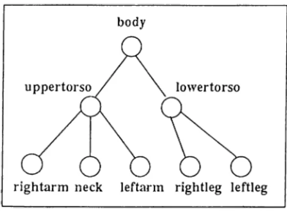
Figure 2.1. Structure of a Model

the modeler connects those base segments with each other as specified in the joint definitions. The connection of segments to each other is of great importance. That is, for a realistic animation the segments of a model should act meaningfully in any kind of orientation. If a segment looks unrealistic in some orientation, it means the joint structure of the model is not planned carefully enough. In fact, each model has a different nature of segment connection and the problem of modeling the joints in a realistic way is a topic of importance in computer animation.

The models of the Mars system consist of joints connected to each other and their base segments defining the shape of the model.

2.1

J o in ts

The joints form an n-ary tree structure (Figure 2.1), i.e. there is no limit on the number of child joints of a joint (so, we can define caterpillars!). Each joint has a parent joint and n children. Two vectors are used to define the X and Y - axis of the joint. The Z - axis is the vector product of X and Y - axis of that joint.

A joint can be rotated about each of its local Xj Y and Z axes, thus has up to three degrees of freedom. This is actually the most ideal situation, but most joints cannot move in each of the three axes. For the sake of ease-of-realism from the animator’s point of view, an upper and a lower limit are specified for the rotation of the joints about each axis. Consequently, a joint may be restricted to one or two degrees of freedom by permitting the joint to rotate about only one or two of the

CHAPTER 2. MARS MODELER

Figure 2.2. A joint rotates with its coordinate axes

axes. Using this method, simple joints, such as fingers (hinge joints), and complex joints such as shoulders (ball-and-socket joints) can be simulated. Also, each joint has its own coordinate axis, which is given in the definition of the model. Most of the time, the Z axis is along the direction of the segment as a convention, but this can be modified to suit the needs of the animator.

As a joint is rotated along its coordinate axes, the axes are also rotated, so it does not matter what the orientation of the joint with respect to the world coordinate axes is. The local coordinate axes are always aligned in the same way with respect to the segment (Figure 2.2).

2.2

S eg m e n ts

Each joint has a base segment that is defined with respect to its local coordinate axis. Detailed, realistic looking models are always preferred and desired in computer animation but the animator does not want to mess with those detailed models while planning the motion. Detailed models are difficult to manipulate. It takes more time to orient a complex model than a simpler one. Mars has a multi representation of the models: one real and others simpler representations. To achieve this, segments of a Mars model are defined as Bezier surfaces [9, 21, 22, 26]^ but instead of directly giving a set of Bezier control points for each segment, the user first defines the

CHAPTER 2. MARS MODELER

Figure 2.3. The sbEs of a model and the actual model

segment bounding box (sbb) of the segment, which is simply the rectangular prism

that bounds the segment itself, and then a set of Bezier control points which are in normalized form. The Bezier control points are defined in a unit cube so that all the points have coordinates with values between 0 and 1.

Eventually this normalized segment definition is scaled with respect to the defined

sbb. If no sbb is defined, a unit cube is assumed (Figure 2.3). As each segment's sbb is defined, we use this simpler representation in the positioning and previewing

phases. This speeds up the respective processes.

For each frame of a film, a transformation matrix is kept for each segment of each model (Figure 2.4).

This matrix is generated from the local and the world coordinate axes and the joint positions. It is updated at every frame should the segment change its place or orientation [25].

2.3

M o d ifyin g a M od el

To create a model, we scale the normalized base segment definitions so that the segment fits into the segment’s sbb. If one changes the dimensions of an sbb without changing its Bezier control points, a new model would be created. It then becomes straight forward to create many models from the same segment definitions. Changing the dimensions of the sbbs and the directions of the local coordinate axes of the model, the base segment is sheared, j'esulting in a number of different models created from

CHAPTER 2, MARS MODELER

p

Transformation

P

world

_Matrix

local

X

World Coordinate Axes

Figure 2.4. Transformation matrix kept for each segment

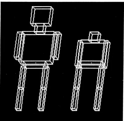
the same normalized segment definitions. This gives us flexibility in creating our models. Creating just one set of Bezier control points^ representing a speciflc segment (e.g. human torso), would be enough to create many types of human bodies (Figure 2.5).

2.4

A n im a tio n -P r e v ie w M od el

Type

Mars uses a simpler representation of the model during the motion planning phase, so that extensive calculations need not be done to position and orient the models. The animator can interactively change the position and orientation of the model and see it instantly. Then, when the keyframes are prepared, he can view the whole motion in real time. He can frequently switch back and fortli between the positioning and previewing phases without having to wait for long minutes for the computer to calculate the inbetween positions of the complex model.

The animator has three choices for the simpler model :

• stick model

• control vertex model rectangular prism model

CHAPTER 2. MARS MODELER

Figure 2.5. Two different models created from the same segments witli different parameters

CHAPTER 2. MARS MODELER

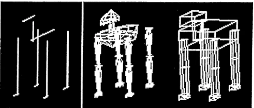
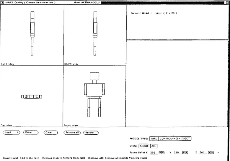
Figure 2.6. Stick, Control vertex, and Rectangular Prism

The stick model is simply a wire man, the control vertex model is composed of the interconnection of the control vertices of the model data and the rectangular prism model is a com])osition of rectangular prisms of the .sbbs of each joint (Figure 2.6). While choosing the models through interactive menus, the animator can view the model from many directions. The model selection screen of Mars can be seen in Figure 2.7. The animator can view the model in any of the three rej)resentations. The representation of the model for the previewing and keyframing should be chosen according to the needs of the models and the animation scene. If real-time playback is achieved by using the control-vertex representation, the animator can clearly see the animation characters and the scene. If flickers occur during playl)ack with the control vertex model, then a simpler representation should be chosen in order to view the animation clearly. Timing is very important in an animation because of the issues like anticipation, staging, slow in and out and etc. The success of an animation de])ends wholly on the timing arrangements of the animator, so the animator should have a strict control on timing.

CHAPTER 2. MARS MODELER

T ) M Ans CasUng ( Choose the ch ara cters ) Murat A KTlJtA N O G LU 0

Le-ft vle^f

□TC I T P ID

R ig h t vle^r

1 ” 1

C c T Y ^ it Model : rdoot ( Z = 50 )

'lo a d ( Draw (Clea.»· ") ( Remove alT) ( Return ^

M O D E L T Y P E ; WIRE CO M TR O L-M ESH R E CT

VIEW : SINGLE ALL

F o c u s P o in t X 2 5 § _ E Q Y 2 30 Z 500 (Load Model : Add to the casO (Rem ove Model : Remove from ca$.0 (Remove A ll : Remove all models from the stack)

C h a p te r 3

A N IM A T IO N

Animation is to give a series of pictures the feeling of motion by using the persistence of vision phenomenon of the human eye. The lower limit for the eye to perceive a series of pictures as continuous is 15 pictures/second. Below this rate, the eye can detect each picture separately. Above this limit, human eye perceive a sequence of still pictures as continuous and moving. Those series of pictures can also be thought of as samples of a real motion taken at regular intervals.

Traditional animators started to use computers first in the painting of drawings. To do this, all the pencil drawings were being scanned into the memory of the computer and then the lines were being enhanced and painted by very simple seed- fill algorithms. Usage of computers has speeded up the preparation of animations so much that, animators started thinking about employing those perfect partners more in the process of animation preparation as inbetweeners. Inbetweeners were those people who drew the inbetweens from the drawings of the chief-animators and painted them. There were so many faults most of the time, either some paint leaped over the line or the inbetween did not look realistic.

This led to the development of tools that produced the inbetweens from the drawings given by the chief-animator. This process is called 2D inbetweening. 2D inbetweening always caused deformations because the information given to the com­ puter lacked one dimension (Figure 3.1).

The thought of giving the computer the 3D definition of the characters wa5 the next step. This has been done by means of the algorithms th at could produce the

CHAPTERS. ANIMATION

2D inbetweening will produce defomiations.

Figure 3.1. 2D Inbetweeiiing

2D view of scene by applying some rendering techniques ( hidden surface elimination and shading) to the 3D data. Also, by the use of homogeneous coordinate systems, fast matrix operations were introduced, to apply rotatiojis and translations to the 3D data of the animation characters. Those developments led to the result that computers started producing meaningful inbetweens from the given 3D keyframes (keyframes are those frames prepared by the chief-animator).

However, there were further problems. There were many possibihties and tech­ niques to make a character move on the computer screen, or to display a series of frames.

3.1

D isp la y T ech n iq u es

The frames of an animation can be displayed on the screen of a computer in one of the three ways:

Read from disk and display

Frames of the animation can be rendered and stored on a storage medium, to be displayed later on. Another program reads those frames from the storage one by one and display them on the screen. Very fast-access disk-drives can reach the 25 frames

CHAPTERS, ANIMATION

per second speed, which is the default value for the PAL system ( 30 frames per second for NTSC system). Storing only the differences between frames may speed up this process.

Frame Buffer Anim ation

Frames, which are rendered and stored on a storage medium can be read into the memory and can be displayed from the memory, which can write to a screen faster than directly from storage medium. But it is obvious that only short sequences of frames can be shown this way, as RAM sizes are small compared to the size of a frame. Using very large random access memories, this technique can be employed. There are special hardware designed to do frame buffer animations like AbekasGOOO^

R ealtim e

The other way is to render the frames and show them instantaneously on the screen. To use this technique, one should use either very simple shading models and algo­ rithms or very fast graphics-devoted machines. Because of the necessity to render each frame in less than a 1/25^^^ of a second, this is most of the time reserved for applications with very simple shading requirements. Flight simulators are a good ex­ ample for real-time display animations. They use flat shading and very sophisticated graphics devoted computers.

3.2

A n im a tio n T ech n iq u es

As computer science and computer graphics techniques improved, many animation techniques other than keyframe animation has been put into use [1, 2, 3, 4, 7, 11, 14, 19, 23, 27]. These techniques are:

Algorithmic Animation

- Kinematic Algorithmic Animation - Dynamic Algorithmic Animation

CHAPTERS. ANIMATION

• Goal-directed Animation

- Goal-directed animation by kinematic laws - Goal-directed animation by dynamic laws • Procedural Animation

• Keyframe Animation

- Image ba.sed interpolative animation - Semi goal-directed keyframe animation - Joint parameters interpolative animation

3 .2 .1 A l g o r i t h m i c A n i m a t i o n

Most phenomena can be successfully animated using abstract motion specification methods, like keyframing, etc. When an animator wants to animate an elastic ball hitting a wall and bouncing back, he has to work very hard to make the whole sequence look realistic. Usually the timing, which is required for a realistic animation, is very hard to achieve manually.

Algorithmic animation is a method that is developed to achieve the realistic animation of physical phenomena of which laws are well defined. Motion specification is done algorithmically, in which physical laws are applied to the parameters of the animated characters. We can classify algorithmic animation system into two as applying kinematic physical laws and as applying dynamic physical laws to the characters. But sometimes the system can admit laws which is apparently specified by the animator, that is the physical laws of the animator.

K inem atic Algorithmic Anim ation

The algorithmic animation systems which use kinematic laws are called the kine­ matic algorithmic animation systems. In this type of motion specification strategy, the animator assigns an initial velocity and an initial acceleration to the animation character or any segment of it. The laws used are;

CHAPTERS. ANIMATION

17

x = v * i = a*f r

where x is the distance taken by the object, i is the time, v is the velocity and a is the acceleration of the object.

By using those laws, functions which specify the trajectories of the animation characters are found and employed in the animation.

The kinematic laws usually produce acceptable but not very realistic motions. They are used when computation time has to be short and dynamic laws cannot be employed.

D y n a m ic Algorithmic A nim ation

The algorithmic animation systems which use dynamic laws, in addition to the kine­ matic laws are called the dynamic algorithmic animation systems. In this type of motion specification strategy, the animator assigns an initial force (torque) to the animation characters or any segment of it. Each segment of each character has a specified mass and the rules used for animating the characters are as follows:

X = a + / “ F = m ^ a

where x is the distance taken by the object, i is the time, F is the force applied on the object, m is the mass and a is the acceleration of the object.

This kind of motion specification is very expensive in terms of processing time and it is only used when strict reahsm is needed. The results are highly remarkable. The bouncing of an elastic ball can only be successfully animated through the use of such dynamic rules.

3 .2 .2 G o a l- d ir e c te d A n i m a t i o n

Sometimes the motion that the animator wants to create is a very specific motion that can be specified to the machine by simple English-like commands hke walk, sit, nod, jump, run.

CHAPTERS, ANIMATION

If the animation program is equipped with a strong knowledge-base, it can per­ form those actions by simple English-like commands. The motion planning and control is done entirely by the machine and the animator only specifies a command.

Usually, a simple command like run is composed of several different actions. What is done is that motion units are defined like lift left leg and those are composed into more complex motion units.

This motion specification method eases the job of the animator, but it also puts strict limits to what the animator can do with the models. If a specific motion is not defined in the knowledge-base, the animator cannot move the models in that way. The quality of a goal-directed animation system depends on the amount of information embedded in the system and how the motion units are implemented. There are two approaches in the implementation of the motion units:

Goal-directed A nim ation by kinematic laws

Goal-directed animation systems that use kinematic motion specification rules are used commonly. Although tliis usually does not give realistic and satisfactory results, its performance superiority over other methods lets the animator produce acceptable results. The basic tools of kinematic motion control are position, displacement, velocity and acceleration of the models.

Goal-directed A nim ation by dynamic laws

Goal-directed animation systems that use dynamic motion specification rules are employed in systems that require high realism. The output of dynamic motion control is highly realistic but it is as much expensive as it is realistic. There is a trade off between realism and computation times.

In dynamic control, energy, force and torque are employed in addition to position, displacement and velocity. The analysis of real physical variables produces very realistic results but the knowledge-base for such a system is huge and the processing time is very long. Real-time animation systems cannot employ such techniques.

CHAPTERS. ANIMATION

3 .2 .3 P r o c e d u r a l A n i m a t i o n

An animation scripting language is used in the specification of motion of the char­ acters. This approach is used in applications where the motion of the models can be procedurally defined.

Examples of such an scripting language is CINEMIRA [10] and ASAS [26] (Actor Script Animation System).

In this approacli the animator writes an program to produce a sequence of ani­ mation. The program is either written in a high level language, and the animation produced through a graphical interface, or it is written in a specially designed ani­ mation scripting system.

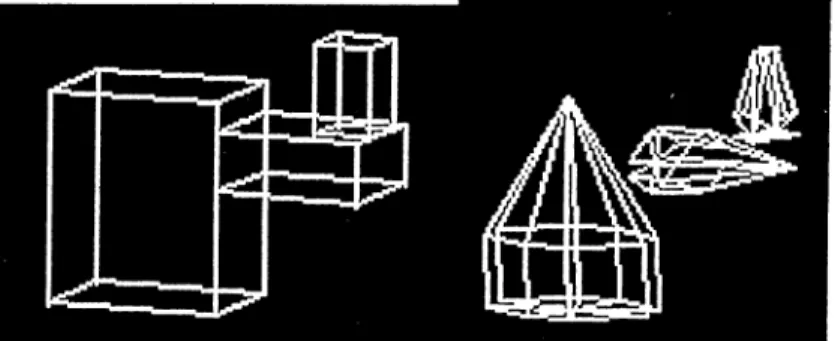
The animator cannot see the result until the script is complete, and this is a major disadvantage. Another disadvantage of this approach is that the effects that will be created by the language cannot be intuitively guessed by the animator, that is the language is very abstract and cannot serve as a user-interactive system. For example the program in Figure 3.2 does not give a good feeling of what will happen in the film.

What the script does is that it spins two cubes on the screen but it is not in­ tuitive. The use of procedural animation is restricted to specific areas, where the animators are experienced programmers and the motions required for the animation are procedurally definable.

3 .2 .4 K e y f r a m e A n i m a t i o n

Keyframe animation is the oldest technique used to generate computer animations. It is adopted from traditional animation. The idea, as referred above, is the same with traditional animation: the animator gives the motion parameters for some specific frames, which are main breakpoints of the desired motion. Then the com­ puter generates the motion parameters for other inbetioeeii It dimes as it has the three

dimensional definitions of the models. There are different techniques in keyframe animation with respect to motion specification or interpolation methodologies to obtain the inbetweens.

CHAPTERS. ANIMATION

(script myprogram

(local: (runtime 96)

(midpoint(half(runtime)))

(animate (cue (at 0)

(start(spin-cube-actor green)))

(cue (at midpoint)

(start(spin-cube-actor blue)))

(cue (at runtime)

(cut))))

Figure 3.2. A sample script

Im a g e based in te rp o la tiv e a n im a tio n

Input to the computer is given as two dimensional pictures and the computer per­ forms two dimensional inbetweening (Figure 3.1). This technique except for some special conditions produces results that are incorrect. Shear effect is observed in the inbet ween frames and models seem distorted. User intervention is needed to achieve a sequence of frames without distortions.

J o i n t p a r a m e t e r s in te rp o la tiv e a n im a tio n

In this approach, the animator specifies the joint parameters of models for some specific frames, which are called keyframes. Then the computer interpolates those joint parameter values and generates the inbetween frames. This approach is very efficient and widely used in computer animation.

CHAPTERS. ANIMATION

Sem i-goal directed keyfram e anim ation

This approach is the same with joint parameters interpolative animation except that the animator specifies the keyframes in a more user-interactive fashion. Бог each keyframe, the animator positions the models by using some simple, English-like commands. This technique is suggested by Ozgiif and Mahmud [IG] and the system developed by this method efficiently melts many approaches in one pot and gives flexibility to the animator in choosing a way to specify the keyframes.

The Mars Animator animates the 3D articulated rigid models using the para­ metric keyframe interpolation method among the many methods in literature.

3.3

M otion Specification

Motion control has always been a problem in computer animation, as the data to be manipulated is 3D and our tools ( mice, digitizers, lightpens, cursors) are 2D. Il is very hard for an animator to visualize a 3D object on a 2D screen, and it is even harder for him to manipulate that object by using 2D manipulators.

From aU these points, we conclude that an interactive manipulation of our 3D animation characters is very hard to achieve, but we want to position and orient our characters any way. We have to give keyframes to the computer, so that it produces an animation.

First, it would be better to examine the criteria of control, that an animator would like to have over the 3D d ata of the animation characters. The animator should be able to apply

• translations to the characters

• rotations (about any of the 3 fundamental axes) to the characters

• rotations (about any of the 3 fundamental axes) to the segments of the char­ acters

There are many possibilities for achieving those criteria. The computer may be loaded with a knowledge base (as with goal-directed approach) and the animation

CHAPTERS. ANIMATION

may be abstracted from the low-level details of the transformation, or the anima­ tor may be required to go into the depths of the motion specification and do the transformation at a very low level.

Indeed, there is a trade-off between high and low-level motion specification schemes. As the motion specification level gets higher, computer does more job, the anim ator’s job gets easier, but the anim ator’s control over the characters is re­ duced. As the motion specification level gets lower, the computer does less job, the animator works more, but his control over the characters increases.

In Mars, we chose a way in between: Joint parameters manipulation. The trans­ lations and rotations are performed as follows:

T ranslation :

To translate an object, a new coordinate:

^ new '> ^VllGW '>

is needed. and can be obtained by the mouse, and we obtain Pzy,^^ by using a slider. As those parameters are chosen by mouse and slider, the object is moved to its new position.

R otation :

To rotate a segment of an model or the model itself (which is the main segment of the model), a quadruple of the form:

R = (^modelname^segmentname^ axis^Q)

is needed. Modelname is the name of the model, segmentname is the name of the segment of the model, axis is either of the three fundamental axes x^y^z and 0 is the rotation angle about this specified axis.

Modelname is selected interactively from the screen. 0 is selected by using a slider. Axis is selected by an exclusive toggle menu. The rotation is applied to

CHAPTERS. ANIMATION

the model with the given modeliiame, axis and 0 as the segment is selected from a pop-up menu. The instance of choosing a segment from the segments pop-up menu can be seen in Figure 3.3. This way. many segments can be rotated with the same parameters consecutively.

Full control of the motion of the models is given to the animator. Each segment can rotate along any of the three axes and by this method, all joints can access any point in 3D space. The animator can create any alignment position of the models by selecting each joint one by one and rotating them.

3.4

Interpolation

When all keyframes are ready, the computer interpolates the parameters of the joints of each model and creates the frames between the keyframes. This is done by an in­ terpolation scheme that depends mainly on the matrix operations. This interpolation is performed as shown in Figure 3.4.

In fact, what is done is tliat, we find the matrix that transforms the first position to the final position. Then from this transformation matrix, a rotation axis and a rotation angle are found. After this angle is divided into the number of inbetween frames, a new transformation m atrix is formed from these axes and the rotation angle step. The details of this process is as follows:

An animation tool should find the inbetween positions and orientations of a moving segment fast and correct. In our implementation of Afars, we have used a mathematically-based approach to find the transformation matrices for the inbe­ tween positions.

In Mars, every segment has a transformation matrix th at transforms the local defined segment points to the world coordinates for each keyframe. Each segment is defined in a local coordinate axis to ease the manipulation of the shape of the models. Also, a defined segment can be used in many orientations and sizes in many models.

Let the local defined points be Piocal their projections onto the screen with re­ spect to the world coordinates be Pworid· The transformation matrix that transforms

CHAPTER 3. ANIMATION

CHAPTER 3. ANIMATION

Pxuorld — localtoHuorId * P lo c a l

for any frame. Note that Piocal does not change throughout the film (if some morpli is not employed in tlie film!).

We want to find the inbetween positions for two points with a known step size

N . We have all the transformation matrices of all segments of all models for each

keyframe. Let us consider a specific interval that is to be interpolated. Let the starting keyframe have the label s and the final keyframe / .

The starting position is given by ^^^d the final position is given by

/local/world· From those two matrices, we can find the transformation m atrix th at

transforms starting position to the final one. It is given by

^ local/local '^'^ / world/local ^ ^ local ^ world

We know M,_^local^world, and as those transformation matrices are orthogonal,

/world/local /local/world / uocal J world

Using this 4x4 homogeneous coordinates transformation matrix -^^^5,000///oca/> can find the axis and the angle of this transformation which can be seen in Figure 3.5.

The angle 0 of the transformation is given by:

0 — cos {{i'l'CLCci^Adij^ans/ormaiion^ ~~ 1)/^)

This angle obviously can take infinitely many values but we chose the smallest positive value as a convention.

Then the arbitrary axis around which the rotation is done is found first by finding the 4x4 vector matrix K:

CHAPTERS. ANIMATION

Then the column matrix k is found from K and finally the column vector n (the axis of rotation) is found by:

n = k / s i n { Q )

After finding the arbitrary axis and the rotation angle, we divide the rota­

tion angle by frame number of first keyframe minus the frame number of the next keyframe, to find the step rotation angle Qstep- The step transformation matrix

MiransJormalion,tep foUlld by:

^^trans Jorviation,tcp = COs(Q^tap) * / + (1 - COs(Qstep)) * 71 * 71^ + Sİ7l{Qstep) * N

All the transformation matrices in that interval are updated using this step trans­ formation matrix.

3.5

Previewing

When the transformation matrices for all the segments of all models for all frames are found, the sequence of animated frames becomes ready to be viewed by the animator. The interpolation and previewing screen of Mars can be seen in Figure 3.6.

Tlie player draws each frame on the screen consecutively one by öne. For this process, it makes many m atrix multiplications of the form:

^world ~ ^'^iransformation * Plocal

for each point of the model. If these multiphcations are done for a complex model with many points, the animation on the screen would be very slow and does not give the feeling of moving models.

Instead Mars uses one of the three skeleton views according to the needs of the animator. This way, real-time playback can be achieved. The modes of the preview model type has been explained in the Modeling chapter.

CHAPTER 3. ANIMATION

0 MAH33tage HehearsW ( K a y Xi^·3c n p t) Mural A K TIH A H O G LU _a

Tco view

R iç tit vievf

P e rs p e c tIv e v l

C u rre n t Model : r i p c i k t l ( Z » 240 )

( C l e a r c a n v a i ) ( I n t e r p e l a n ) ( S e e f i l m ~ ~ )

Save Iilm ^ F ile n a m e : ;mr _f un ^R etu rn ^

( R e c o r d M o d e l s ' )

M O D E L T Y P E : I W I R E | C O N T R O L - H E S H | R E C T |

VIEW : SIN GLE ALL

Fo c u s P o In t X 25§ ^ Q 3 Y 236 Z 500 I ^ F I

CHAPTERS. ANIMATION

The benefit of choosing a multi representation becomes clear at this stage. The anim ator can view the created motion in real time, so editing is easier and faster. By means of this preview phase, the animator can see the created motion and make changes, before the long process of rendering begins.

Up to the previewing phase, the model is treated with its stick, control points or sbb representations. At this stage, the Mars animator creates the Bezier surfaces from the control points or directly reads the patch definitions of segments from file.

After editing, when the desired motion sequence is achieved. Mars sends the model’s data and the motion data to the multicomputer for rendering of the scene.

3.6

Communication between the Animator and the Ren-

derer

After all the previewing is done and the desired motion sequence is achieved, the scenes get ready to be rendered. This expensive process is done on a multicomputer, to cut down the total film-making process. This means that the data representing the models and the animation should be transm itted to the multicomputer in an appropriate form.

After previewing, we have the model data and the motion sequence data. The im portant point in this stage is the way this model and motion data is communicated between the Animator and the Renderer. There are a number of ways to.do this. The criterion of optimized communication is that this data should be well compressed and it should have no redundancy as well as containing all the necessary information about the models used and the specifications of the motion.

The format of this data is very significant. There is a trade off between the data size and the data interpretation time. If the animator sends the data to the renderer in a very compact form, it takes more time for the renderer to achieve the data. For example, the data for the inbetween frames which the animator ha^ might be omitted from the communication packet because the renderer can find those values by itself if it is given the necessary database. This obviously increases the processing time of the renderer and since the animator already has this data, it would take less time for the renderer to read it from file than compute itself. So, we have to be careful

CHAPTERS. ANIMATION

Figure 3.7. Data formats for communication

about what to insert into and what to omit from this data. The communication format of Mars is shown in Figure 3.7. The model data communication is straight forward. Each model has some segments, and each segment has its own definition. But for motion data, the transformation matrices for each segment of each model is communicated only for the first frame of the film. Then, a transformation matrix of a segment is transm itted to the multicomputer if the segment has changed its place or orientation since the previous frame. This provides a significant compression of data since only the necessary matrices are transm itted. This is also exploited in the processing of data, as will be seen in the next section.

C h a p te r 4

R E N D E R IN G

Rendering is the process of producing realistic images or pictures. Visual perception involves mainly physics and positioning of the surfaces and objects observed. In the rendering process of a three-dimensional scene that is composed of three-dimensional objects and surfaces, two issues are considered: how the surfaces reflect the incident bght, th at is the illumination model of the objects and which surfaces and objects are seen and which are hidden.

4.1

Illumination Model

When light energy falls on a surface, it can be absorbed, reflected or transmitted. It is the reflected or the transmitted light that makes a surface visible. W hat makes us see an object colored is that some wavelengths of the incident light may be absorbed more than other wavelengths. When a white light falls on a surface and red and green components of the light is absorbed by the surface, the surface is visually percepted as blue. To give this effect computationally in computer generated pictures, there are mainly two illumination models used by the computer scientists: P h o n g [5] and C o o k -T o rra n c e [20] illumination models.

Phong model is an illumination model that deals with only a few illumination parameters, but yet stiU gives acceptable results. Another model, the C ook an d T o rra n c e illumination model is a more realistic model. It deals with a lot of pa­ rameters bke the Fresnel term, attenuation factor, surface distribution function and

CHAPTER 4. RENDERING

the non-uniform reflectance hemisphere o f the surface. As the Cook and Torrance model is a more physically-based model than the Phong model, which is roughly an approximation of the former, it requires more computations than the Phong model. The more complex the illumination model is, the more expensive the computations but the more realistic our pictures are. More realistic pictures are always justified in computer graphics but after all, Phong shading model is used almost all the time instead of Cook and Torrance model which is very expensive. Phong model provides realism enough to avoid all those parameters. In our implementation of rendering a sequence of animated film frames, we have used Phong’s algorithm.

4.2

Hidden Surface Removal

For rendering a scene, first the liidden surfaces should be removed, and the projection of the scene onto the two dimensional screen must be performed. This process also includes the rasterization on the projected surfaces.

A comparison of hidden surface removal algorithms may be found in [24]. In this survey, hidden surface removal algorithms are classified as operating on object-space or the image-space, and the degree of cohei'cnce they employ. Here coherence means the processing of geometrical units, such as areas or scan line segments, instead of single pixels.

There are currently two popular approaches to hidden surface removal: Z-bufFer based systems and scan line based systems. Other approaches like area subdivision or depth-list schemes are not extensively used and they are only reserved for special- purpose applications like flight simulators.

The Z-buffer algorithm developed by Catmull [8], combined with the Phong re­ flection model represents the most popular rendering scheme. This algorithm, using Sutherland’s classification scheme, works on image-space or screen-space.

Pixels in the interior of a polygon are shaded by an incremental shading technique and their depths are evaluated by interpolation from the z values of the polygon vertices. For each pixel the nearest visible point is buffered and compared to the next coming point, which is projected onto the same pixel (Figure 4.1).

CHAPTER 4, RENDERING

There is a variation of the Z-bufFer algorithm for use with scan line based sys­ tems, whicli is called scan line Z-buffer. The rendering method, Mars uses is scan

lijie Z-buffer hidden surface removal algorithm [26]. This algorithm consists of two

phases. In the first phase, the algorithm goes through all the polygons in the scene to find and store the intersection points of each polygon with the scanlines of the image. Hence, the first phase effectively constructs a one-dimensional array of point­ ers scanlines scanlines(i) Y>omis to the linked list that contains the edgeboxes

on the i^^^ scanline (Figure 4.8). In the second phase, scanlines are processed one after another. In each scanline, the segments indicated by the edgeboxes in the cor­ responding linked list are rendered. All the pixels between two intersection points are shaded with Phong shading model and with an incremental shading technique. There are two approaches to calculate the intensities of the pixels, that lay between the two edgebox pixels. The first one, which is called Gouraud interpolation, is to calculate the intensities at the edges and then bnearly interpolating those intensities for the inbetween pixels. The second approach, which is called Phong interpola­ tion, is to interpolate the normals linearly for each inbetween pixel and calculate the intensity value afterwards. The second approach is apparently more expensive than the first one, but generally, more expensive methods generate realistic looking

CHAPTER 4. RENDERING

pictures. Phong interpolation generates highlights that look more realistic, while Gouraud interpolation results are narrower. Mars uses Phong interpolation, because realistic looking pictures form realistic animations after all.

We have preferred this algorithm mainly due to its very special nature that perfectly suits our tools of optimizing the rendering process. It first runs on the object-space and then the image space. Moreover it requires much less memory than conventional Z-buffer algorithms that holds all the screen space for the rendering. Scan line Z-buffer hidden surface removal algorithm is easy to implement, but as each pixel of each patch is visited, it is compu-tationally expensive. The speed of this algorithm is the bottleneck of all the film-making process.

Of the three phases, rendering has attracted the most attention and research. More efficient techniques were needed to be developed to make the images look more realistic and to finish the overall process in a shorter amount of time.

If we think of rendering a picture as reducing a 3D scene to a 2D image, then the rendering of an ani!n?J:ed film, i.e. a sequence of fram.es, is reducing a 4D scene (including time as the fourth dimension) to a 3D image (a series of frames, including time as the third dimension). Thus, rendering an animated sequence of frames must be thought differently than the rendering of a static scene. Hence, rendering a scene and a film are considerably different processes.

If we do the rendering of a sequence of animated frames separately, i.e. render each frame as totally irrelevant to each other, the result would be acceptable, but there are surely better ways to do this, as long as the sequence of frames has a very im portant characteristic that must be thought of. In terms of efficiency of processing, what makes a sequence of animated film frames different from a sequence of totally irrelevant frames is the concept of temporal coherence [26].

4.3

Temporal Coherence

Any object or joint in an animated film has a great degree of coherence between successive frames. That is to say, in consecutive frames, an object or a joint makes a relative translation or a rotation to its previous position and orientation [13].

CHAPTER 4. REhWERING

c = ^ l

Figure 4.2. High degree of coherence in a film

should fully exploit the tem})oral coherence between successive frames in order to reduce the rendering job. It should avoid rendering the parts of the picture that do not change after the ])revious frame. Such an algorithm should have a buffering

mechanism tliat buffers the parts of the ])icture that 4n not change and parts of

the picture that will change in the next frame. After rendering a frame totally, creating the next frame can be done by simply rendering only those parts of data that have changed their place and orientatioîi since the i)revious frame. The basis of such an algorithm is the coherence between successive frames of an animated film (for an example see Figure 4.2). Temporal coherence is one phenomena exploited fully to render animated film sequences more efficiently. As long as efficiency is our main academic goal, we must think also of oi)timizing our conventional sequential rendering algorithm. As will be seen in the Algorithm section, it is optimized to its best in terms of sequential ])rocessing but there is still something more we can do :

parallel processing.

4.4

Parallel Processing

In literature, there are several works done on parallel rendering of a scene [2(S]. Most of the studies have a great dependency on the nature of the parallel architecture employed. The architecture we have implemented our algorithm on is Intel’s iPSC/2 hypercube. iPSC/2 is a distributed memory and message-passing multicomputer. The iPSC/2 we are currently using ha.s 32 processors. We have tried to improve an algorithm that would give good results on other parallel machines as well.

CHAPTER 4. RENDERING

Figure 4.3. Screen space subdivision

4.5

The Algorithm

The algorithm to render the sequence of animated frames mainly depends on the temporal coherence and parallelism concepts and it is based on a modification of the conventional scan line Z-biiffer hidden surface removal algorithm.

If we modify the Z-buffer algorithm such that, first all the patches are processed to form the edgeboxes, and then this heap of edgeboxes is processed to generate the intensity values, it becomes an algorithm that runs first in object space and then in the image (screen) space. This is the most im portant part of the parallel algorithm. The subdivision problem will be solved with the addressed concept.

Load balance is one of the main goals in parallel algorithm design process, but to achieve load balance in the rendering process of a scene, composed of 3D objects, the distribution of the objects th at consist of patches to the processors is a critical job. Most of the time some assumptions and approximations are made.

There are mainly two approaches to the load distribution problem. One of them is screen (image) space subdivision and the other is object space subdivision.