A goal programming approach to mixed-model assembly line balancing problem

(1)

produhtion

economics

ELSEVIER Int. J. Production Economics 48 (1997) 177-185

A goal programming approach to mixed-model assembly line

balancing problem

Hadi Gokce+*,

Erdal Erelb

“Industrial Engineering Department, Gazi University Maltepe 06570 Ankara, Turkey bFaculty of Business Administration, Bilkent University. Bilkent 06533 Ankara, Turkey

Received 16 February 1995; accepted 27 June 1996

Abstract

In this paper, a binary goal programming model for the mixed-model assembly line balancing (ALB) problem is developed. The model is based on the concepts developed by Patterson and Albracht [l] and the model of Deckro and Rangachari [2] developed for the single-model ALB problem. The proposed model provides a considerable amount of flexibility to the decision maker since several conflicting goals can be simultaneously considered.

Keywords: Assembly line balancing; Goal programming

1. Introduction

Assembly line balancing (ALB) has been a focus of interest to the production/operations manage- ment community for the last 40 years. The classical ALB problem was first described in 1955 by Salveson [3], who presented a mathematical formulation of the problem and suggested a solution procedure. Since that time, several techniques have been proposed for the solution of the ALB problem; see the review papers of Baybars [4] and Ghosh and Gagnon [S]. Although there are numer- ous studies published on the various aspects of the problem, the number of studies on the mixed-model assembly lines are relatively small. The complex mathematical nature of the problem hinders the attempts to obtain solution procedures. However

* Corresponding author.

today, an increasing number of firms are using mixed-model assembly lines to cope with the pres- sure of producing several models to attain higher customer satisfaction without holding large stocks of finished goods.

ALB problems are traditionally formulated and solved with the objective of either the minimization of cycle time or the minimization of the number of stations utilized along the line. However, ALB problems, in practice, are typically associated with different and usually conflicting objectives such as cycle time, number of stations, workload differ- ences between stations, plant layout requirements, etc. In the literature, a few reported studies have utilized a multiple criteria approach to the ALB problem; Gunther et al. [6] first proposed a goal programming model for the ALB problem and presented a solution procedure using a goal priori- tized branch-and-bound scheme. Deckro [7] has developed a model which simultaneously considered

(2)

178 H. Gokcen, E. ErelJInt. J. Production Economics 48 (1997) 177-185

the minimization of cycle time and the number of stations. Malakooti [8] has formulated the ALB problem as a multiple criteria problem where several objectives and constraints are defined, and has developed an interactive multiple criteria decision making (MCDM) approach for solving the problem. Deckro and Rangachari [2] have developed an alternative goal programming formulation which can accommodate the Gunther et al. [6] goals in addition to various other goal constraints. Lastly Malakooti [9] has formulated the ALB problem with buffers as a single criterion decision making as well as a MCDM problem. All the MCDM literature described above are concerned with the single-model ALB problem and, to the best knowledge of the authors, there has not been any published study dealing with the multiple criteria aspects of the mixed-model ALB problem so far.

Formally, a mixed model ALB problem can be stated as follows: Given P models, the set of tasks associated with each model, the performance times of the tasks, and the set of precedence relations which specify the permissible orderings of the tasks for each model, the problem is to assign the tasks to an ordered sequence of stations such that the precedence relations of each model are satisfied and some performance measures are optimized. Unlike the single-model line, different models of a product are assembled on a mixed-model assembly line; the models are launched to the line one after another.

This paper presents a binary goal programming model for the mixed-model ALB problem. A goal programming approach would seem to be a natural modelling tool and a more realistic approach for the ALB problem, since goal programming attempts to achieve a “satisfactory” rather than the “optimal” solution in the face of conflicting goals. The proposed model in this paper provides a considerable amount of flexibility to the decision maker since several goals of which some may be conflicting with each other, can simultaneously be considered.

The paper is organized as follows. Section 2 presents the notation and the assumptions of the model. The goal programming formulation is developed in Section 3. Solutions of some example problems are presented in Section 4. Finally, the paper concludes with a summary of the approach.

2. Notation and assumptions

The goal programming model utilizes some of the concepts developed by Patterson and Albracht [l] for a single-model ALB problem and the integer programming formulation of Gokcen [lo] for the mixed-model ALB problem. In addition, some of the goal constraints of the model of Deckro and Rangachari [2] for the single-model ALB problem have been utilized.

The notation used in the formulation is as follows: N K P PRi si 4, G & Li X km Ak

total number of tasks in the problem number of stations

number of models (products)

subset of all tasks that precedes task i, i=l 2 ... 9 N

subset of all tasks that follow task i, i = l,...,N

performance time of task i of model m, i=l ,..., N, m = l,..., P

cycle time of model m, m = 1, . . . , P earliest station to which task i can be assigned given the precedence relations, i=l , ... 7 N

latest station to which task i can be assigned given the precedence relations, i = l,...,N

1 if task i is assigned to station k; 0 other- wise, i= l,..., N, k= l,..., K

1 if station k is utilized for model m; 0 otherwise, k = 1, . . . , K, m = 1, . . . , P

1 if station k is utilized by all models; 0 otherwise, k = 1, . . . , K

subset of all tasks that can be assigned to station k of model m, k = 1, . . . ,K, m = l,...,P

11 wk,,,II number of tasks in Set wk,, k = 1, . . . ,K, m = 1, . . ..P

The assumptions of the model are listed below: 1. Similar models are produced on the same production line.

2. Task performance times of each model are known constants.

3. Precedence diagrams of the models are known.

4. No WIP inventory buffer is allowed between stations.

(3)

H. Gokcen, E. Erel/Int. J. Production Economics 48 (1997) 177-185 119 5. Common tasks of different models must be

assigned to the same stations.

6. Number of stations are the same for all models. 7. Parallel stations are not allowed.

Typically there are several tasks common to the various models manufactured on a mixed-model assembly line. Thus, the precedence diagrams of the models can be combined into a unique diagram. Thomopoulos [ 1 l] used the concept of a combined precedence diagram to transform different models into an equivalent single model. The combined diagram is constructed by taking the union of the

P--Y

\

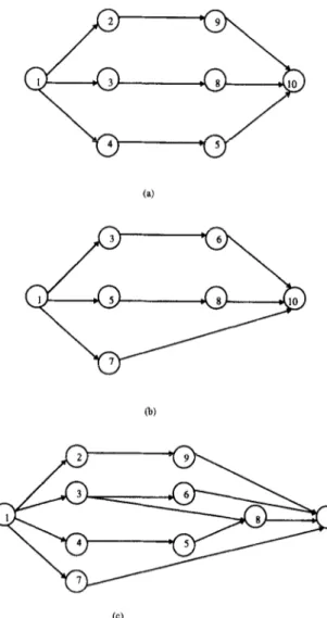
Fig. 1. Precedence diagrams for (a) model 1, (b) model 2, and (c) the combined diagram.

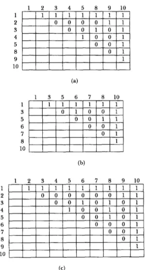
nodes and the precedence relations of the diagrams of all the models. The construction of the combined diagram is straightforward with precedence matrices; a precedence matrix is an upper-triangular matrix with the abth entry equal to 1 if the process- ing of task b requires the completion of task a. Otherwise the entry is zero. In the precedence matrix of the combined diagram, the abth entry is equal to 1 if the abth entry of any of the precedence matrices of the models is equal to 1; additionally, some abth entries that are initially zero may finally be 1 due to implied precedence relations. For example, in the combined diagram, if acth and cbth entries are both 1 with a zero for the abth entry, then the ubth entry should be changed to 1. Note that there should be no conflict in the precedence relations across the models; for example, if a model requires the completion of task a before task b, then no other model should require the completion of task b before task a. A simple example with two models is given in Fig. 1 to illustrate the process of constructing a combined diagram. The numbers within the circles represent tasks and the arrows connecting the circles specify the precedence relations. In Fig. 2, the associated precedence matrices of the diagrams of Fig. 1 are depicted..

The earliest and latest stations task i can be assigned to, given the precedence relations, Ei and Li, respectively, are first developed by Patterson and Albracht [l] for the single-model assembly line balancing problem. These expressions greatly reduce the number of variables in the model; the modified versions of these expressions for the mixed-model assembly line balancing problem below are used in our model.

tim + 1 tjm + Ei = max m=l,...,P [ 1 jsP& cm ’ (1) Gm +

C

tjm + Li= min K + l- [

I

jtSi m= l,...,P _Gn _’ (2)

where [x] + denotes the smallest integer greater than or equal to X. The number of stations, K, can be estimated from the operational setting or heuris- tic procedures shown to perform well; an upper bound on K is N.

(4)

H. Gokcen, E. Erelllnt. J. Production Economics 48 (1997) I77-I85 180 1 2 3 4 5 8 9 10

The calculation of Ei and Li based on an estimate of five stations for the line length and the task performance times of the example in Fig. 1 are given in Table 1.

3. Goal programming formulation

(a) In a preemptive goal programming model, the

1 3 5 6 ‘7 8 10

upper level goals are first optimized before lower level goals are considered. In a nonpreemptive model, the goals are given some weights and considered simultaneously. In this paper, we utilized the preemptive approach due to the difficulty associated with determining the weights for the various goals. 1 3 5 6 7 8 10 (b) 1 2 3 4 5 6 7 8 9 10 (c)

Fig. 2. Precedence matrices of for (a) model 1, (b) model 2, and (c) the combined diagram.

Table 1

Task performance times and Ei and Li values of problem 1 Task (i) Performance Performance Ei Li

time for model 1 time for model 2

1 10 10 1 3 2 4 1 5 3 I 9 1 4 4 7 1 5 5 4 5 1 4 6 12 2 5 7 6 1 5 8 12 13 2 4 9 7 1 5 10 11 10 3 5 3.1. Assignment constraints

This set of constraints guarantees that tasks of each model are assigned to at most one station and can be written as follows:

,sE Kk=l, i=l,..., N. i

The assignment constraints are not suitable for consideration as goals; however, exclusion of a task or multiple assignments of tasks to stations can be implemented easily [7].

3.2. Precedence constraints

We have utilized the precedence relationship of Patterson and Albracht [l] developed for the single-model version. In the combined precedence diagram, the precedence relation between task a and task b, where b is an immediate follower of a, can be expressed as follows:

5 k . V,, - 5 k . V,, < 0 ₍₄₎

k=E. k=Eb

for each pair of tasks a and b where L, > Eb. Similar to the assignment constraints, precedence constraints are not appropriate for consideration as goals [7].

(5)

H. Gokcen, E. Erelllnt. J. Production Economics 48 (1997) 177-185 181

3.3. Cyclic time constraints

The cyclic time constraints assure that summa- tion of task times for each model within a single station is less than or equal to the cycle time of the model. These can be expressed as follows:

iEGk. rim. I& < C,, k = 1, . . . ,K, m = 1, . . . ,P. (5)

The goal constraints for the cycle time can be written as

1 ti,.l/ik+dip-dz=Cm, isW,,

k = l,..., K, m = l,..., P ₍₆₎

The deviational variable, dz, denotes over- achievement of the cycle time for each station for model m. The minimization of d: for each model simultaneously will minimize the cycle times of the models. The deviational variable, d,, denotes the idle time in station k for model m. The minimization of the sum of the d,$ deviational variables will minimize the total idle time.

The difference between the d& deviational variables at each station can be limited to a predeter- mined value, ok, as follows:

k= l,..., K, m= l,..., P- 1, (7)

where wk is the bound on the variation of idle time between models in station k. This constraint can be expressed as a goal by adding the necessary deviational variables; however, a rapid increase in the number of constraints due to the absolute value function is inevitable.

3.4. Zoning constraints

Zoning constraints refer to the undesirability or the desirability of assigning tasks into the same station. The former is called incompatible zoning and the latter is called compatible zoning. For the incompatible zoning constraints, the expression developed by Patterson and Albracht [l] is used. In the combined diagram, incompatible tasks a and b, where a succeeds b, can be expressed as

k=E. k=Eb

This constraint can be expressed as a goal by adding deviational variables as follows [a]:

5 k.l/,,- z k*vbk+dic-d;,=l. ₍₉₎

k=E, k=Eb

The deviational variable, d,,, is used to assure that incompatible tasks cannot be assigned to the same station.

The compatible zoning constraint can be expressed with a small modification in the above expression as follows [7]:

i k . v,, - 5 k . v,, = 0.

k=E, k=Eb

Similar to incompatible zoning, this constraint can also be expressed as a goal by adding deviational variables as follows [2]:

F k.F/,,- F k+‘~,+d,,,-d&,=0. (11)

k=E. k=Eb

If the deviational variables d,,, and d&, are driven to zero, the compatible tasks a and b in the combined diagram will be assigned to the same station.

3.5. Station constraints

Each model utilizes the same number of stations; in other words, if the work content of a station for a specific model is zero, then the work content of this station for all the other models must also be zero. The station constraint developed by Deckro [7] is modified for the mixed-model version as follows:

k= l,..., K, m= l,..., P,

i Xkm-P’I&=o, k=l,..., K. m=l

(12) (13)

Note that with the above expressions, each station is assured to have at least one task from each model. If a specific number of stations, ST, is imposed by the decision maker, we can write the following

(6)

182 H. Gokcen, E. Erelllnt. J. Production Economics 48 (1997) I77-185

constraint:

(14) k=l

This constraint can be expressed as a goal by adding deviational variables as follows:

5 Ak+ds; -d$ =ST. ₍₁₅₎

k=l

The classic objective of minimizing the number of stations utilized along the line can be achieved by maximizing d,: .

4. Illustrative examples

We apply the proposed goal programming model to a mixed-model ALB problem with two models. The precedence diagrams of the models and the combined diagram are depicted in Fig. 1. Note that the combined diagram has 10 tasks, whereas the first and second models have 8 and 7 tasks, respectively. Task performance times for each model, the Ei and Li values are given in Table 1. A reasonable estimate of the number of stations is given as 5.

using GAMS on an IBM 2155-593 computer. Task assignments are shown in Table 2. Three stations are utilized with a cycle time of 23 for both the models. Tasks 1 and 3 are assigned to different stations. In other words, priority 1 and priority 3 are satisfied while priority 2 is unsatisfied.

In sequencing the goals of a preemptive goal programming model with P priority levels, P! different sequences of the goals can be created. In other words, the goals can be ordered in P! different ways. Such an analysis is useful to the decision maker since it serves as a sensitivity analysis tool. The results of the 3! = 6 different sequences of the goals are given in Table 3.

Three goals with priority levels below are used in the formulation:

Goal with priority level 1: number of stations should not exceed 3.

Goal with priority level 2: cycle time should not exceed 22 for model 1 and 24 for model 2.

Goal with priority level 3: tasks 1 and 3 should not be assigned to the same station.

The goal programming formulation of the problem is given in the appendix. The problem is solved

Note that either the priority 1 goal (number of stations limit) or the priority 2 goal (cycle time limit) is not satisfied in each sequence in Table 3. Priority 1 and 2 goals are conflicting goals. The priority 3 goal (incompatible zoning) is always satisfied even when this goal is considered as the last goal (sequences 1 and 3). The above analysis suggests reconsidering the limits imposed by the priority 1 and 2 goals. In other words, the decision maker must accept either a longer cycle time or a larger number of stations.

Table 3

Sensitivity analysis of problem 1 made by changing the order of the goals Table 2

Task assignments of problem 1

Station Tasks Model 1 Model 2 Tasks Station Tasks Station

time time 1 1, 4, 5, 7 1,4,5 21 1,5,7 21 2 2, 3, 6, 9 2, 3, 9 18 3,6 21 3 8, 10 8, 10 23 8, 10 23 Sequence no.

Priority 1 Priority 2 Priority 3 Unsatisfied Value of nonzero Cycle time Number

goal deviational of stations

variables Model 1 Model 2

1 Pl P2 P3 P2 CYCl = 1 23 24 3 2 Pl P3 P2 P2 CYCl = 1 23 24 3 3 P2 Pl P3 Pl STA = 1 22 24 4 4 P2 P3 Pl Pl STA=l 22 24 4 5 P3 P2 Pl Pl STA = 1 22 24 4 6 P3 Pl P2 P2 CYCl = 1 23 24 3

(7)

H. Gokcen, E. Erellht. J. Production Economics 48 (1997) 177-185 183 Table 4

Solutions of problems obtained by adding lower level goals Prob. no. Number of tasks in combined diagram Common task percentage Goals” Solution time (s) 1 2 3 1 10 50 2 20 60 3 30 63 4 40 67

Priority 1: Number of stations goal Priority 2: Cycle time goal

Priority 3: Incompatible zoning goal Priority 1: Cycle time goal

Priority 2: Compatible zoning goal Priority 3: Number of stations goal Priority 1: Cycle time goal Priority 2: Number of stations goal Priority 3: Compatible zoning goal Priority 1: Number of stations goal Priority 2: Incompatible zoning goal Priority 3 Cycle time goal

s U U 1.64 S U U 22.36 S U S 37.13 S U U 9.72 S S U 8.96 S S S 62.01 S U U 30.70 S S U 26.04 S S S 23.56 S S U 5.66 S S U 8.35 S S S 20.87 a S: satisfied; U: unsatisfied.

We have solved three two-model example problems with 20, 30 and 40 number of tasks in the combined diagram, respectively, in addition to the above example. The results along with the lo-task example above are shown in Table 4. The common task percentage column denotes the percentage of the tasks common to both of the models. In the first row of each problem, only the priority 1 goal is considered, in the second row, priority 1 and 2 goals are considered, and in the third row, all of the goals are considered. For example, the third row of problem 1 corresponds to the first sequence in Table 3.

The observations made on this limited number of example problems are as follows: The solution time is highly sensitive to the number of stations goal relative to K; for example, the small solution times of problem 4 are attributable to the relatively large number of stations goal. If a goal of lower priority is satisfied, then there is no need to consider the lower priority goal; such a case exists in the second row of problem 4.

5. Conclusion

In this paper, a goal programming model for the mixed-model ALB problem is suggested. The

model is heavily based on the concepts of earlier researchers [ 1,7,11], and the models developed for the single-model version of the problem [l, 2-J. However, the model is the first MCDM approach to the mixed-model version.

The size of the model can grow rapidly as the problem is NP-hard, since with a single model and tasks with no precedence relations, it is easy to reduce the problem into a bin-packing problem which is NP-hard in the strong sense. However, when a goal was met, it is not necessary to spend computational time to providing optimality. In other words, if the deviational variables at a goal can be minimized to zero, it is not necessary to make further computation for that goal.

Goal programming usually results in a “compro- mise” since the solution provides “satisfactory” levels of performance in terms of conthcting objectives, rather than identifying the “optimal” solution with respect to a single objective. The goal programming model suggested here provides flexibility to the decision maker in evaluating different alternatives.

References

[l] Patterson, J.H. and Albracht, J.J., 1975. Assembly-line balancing: zero-one programming with Fibonacci search. Oper. Res., 23: 166-172.

(8)

H. Gokcen, E. Erelilnt. J. Production Economics 48 (1997) 177-185 184 c21 c31 c41 c51 C61 c71 C81 c91 WI Cl13

Deckro, R.F. and Rangachari, S., 1990. A goal approach to assembly line balancing. Comp. Oper. Res., 17: 509521. Salveson, M.E., 1955. The assembly line balancing problem. J. Ind. Eng., 6: 18-25.

Baybars, I., 1986. A survey of exact algorithms for the simple assembly line balancing problem. Mgmt. Sci., 32: 909-932.

Ghosh, S. and Gagnon, R.J., 1989. A comprehensive literature review and analysis of the design, balancing and scheduling of assembly systems. Int. J. Prod. Res., 27: 637-670.

Gunther, R.E., Johnson, G.D. and Peterson, R.S., 1983. Currently practised formulations for the assembly line balancing problem. J. Oper. Mgmt., 3: 209-221. Deckro, R.F., 1989. Balancing cycle time and worksta- tions. HE Trans., 21: 106-111.

Malakooti, B., 1990. A multiple criteria decision making approach for the assembly line balancing problem. Int. J. Prod. Res., 29: 1979-2001.

Malakooti, B., 1994. Assembly line balancing with buffers by multiple criteria optimization. Int. J. Prod. Res., 32: 2159-2178.

Gokcen, H., 1994. New models for deterministic mixed- model assembly line balancing problems. Unpublished Ph.D. Thesis. Gazi university, Ankara.

Thomopoulos, N.T., 1970. Mixed-model line balancing with smoothed station assignments. Mgmt. Sci., 16: 593-603.

Appendix

Goal programming formulation of the example problem

positive deviational variable of station constraint.

negative deviational variable of station constraint. Deviational Variables STA ISTA CYCl CYC2 ZNG HAk HBk IZNG

positive deviational variable of cycle time constraint for model 1.

positive deviational variable of cycle time constraint for model 2.

negative deviational variable of zoning constraint.

negative deviational variable of cycle time constraint for kth station of model 1. negative deviational variable of cycle time constraint for kth station of model 2. positive deviational variable of zoning constraint.

Model

Min Pl(STA), P2(CYCl + CYC2), P3(ZNG) Subject to Assignment Constraints Vll + v12 + v13 = 1 V21 + V22 + V23 + V24 + V25 = 1 V31 + V32 + V33 + V34 = 1 V41+V42+V43+V44+V45=1 v51 + v52 + v53 + v54 = 1 V62 + V63 -t V64 + V65 = 1 V71 + V72 + V73 + V74 + V75 = 1 V82 + V83 + V84 = 1 V91+ V92 + V93 + V94 + V95 = 1 v103 + v104 + v105 = 1 Precedence Constraints Vll + 2V12 + 3V13 - V21- 2V22 - 3V23 - 4V24 - 5V25 < 0 Vll + 2V12 + 3V13 - V31- 2V32 - 3V33 -4V34dO Vll + 2V12 + 3V13 - V41 - 2V42 - 3V43 - 4v44 - 5v45 < 0 Vll + 2V12 + 3V13 - V71- 2V72 - 3V73 - 4v74 - 5v75 < 0 V21+ 2V22 + 3V23 + 4V24 + 5V25 - V91 - 2V92 - 3V93 - 4V94 - 5V95 < 0 V31 + 2V32 + 3V33 + 4V34 - 2V62 - 3V63 - 4V64 - 5V65 < 0 V31 + 2V32 + 3V33 + 4V34 - 2V82 - 3V83 - 4V84 < 0 V41+ 2V42 + 3V43 + 4V44 + 5V45 - V51 - 27152 - 3V53 - 4V54 < 0 2V62 + 3V63 + 4V64 + 5V65 - 2V103 - 3V104 - 4v105 < 0

(9)

H. Gokcen. E. ErellInt. J. Production Economics 48 (1997) 177-185 185 VSl + 2v52 + 3v53 + 4v54 + 5v55 - 2V82 - 3V83 - 4V84 < 0 3V83 + 3V84 - 3v103 - 4v104 - 5VlO5 < 0 V91 + 2V92 + 3V93 i- 4V94 + 5V95 - 3VlO3 - 4v104 - 5v105 < 0 v71 + 2v72 + 3v73 + 4v14 + 5v15 - 3v103 - 4v104 - 5v105 Q 0

Incompatible Zoning Goal Constraint V31 + 2V32 + 3V33 + 4V34 - Vll - 2V12

- 3V13 + ZNG - IZNG = 1

Cycle time goal constraints (for model 1) lOVl1 + 4V21 + 7V31 + 7V41 + 4V51 + 7V91 + HAl-CYCl = 22 lOV12 + 4V22 + 7V32 + 7V42 + 4V52 + 12V82 + 7V92 + HA2-CYCl = 22 1OV13 + 4V23 + 7V33 + 7V43 + 4V53 + 12V83 + 7V93 + llV103 + HA3-CYCl = 22 4V24 + 7V34 + 7V44 + 4V54 + 12V84 + 7V94 + llV104 + HA4 - CYCl = 22 4V25 + 7V45 + 7V95 + llV105 + HA5 - CYCl = 22

Cycle Time Goal Constraints (for model 2) 1OVll + 9V31 + 5V51 + 6V71 + HBl - CYC2 = 24 lOV12 + 9V32 + 5V52 + 12V62 + 6V72 + 13V82 + HB2 - CYC2 = 24 lOV13 + 9V33 + 5V53 + 12V63 + 6V73 + 13V83 + lOV103 + HB3 - CYC2 = 24 9V34 + 5V54 + 12V64 + 6V74 + 13V84 + lOV104 + HB4 - CYC2 = 24 12V65 + 6V75 + lOV105 + HB5 - CYC2 = 24 Station Constraints Vll + v21 + v31 + v41 + v51 + v91 -6X11 60 V12 + V22 + V32 + V42 + V52 + V82 + V92 - 6X21 < 0 V13 + V23 + V33 + V43 + V53 + V83 + V93 v103 - 8X31 < 0 V24 + V34 + V44 + V54 + V84 + V94 + V104 - 7x41 d 0 V25 + V45 + V95 + V105 - 3X51 6 0 Vll + V31 + V51 + V71 -4X12 < 0 V12 + V32 + V52 + V62 + V72 + V82 - 5X22 < 0 V13 + V33 + V53 + V63 + V73 + V83 + V103 - 7X32 < 0 V34 + V54 + V64 + V74 + V84 + V104 - 6X42 < 0 V65 + V75 + V105 - 2X52 < 0 X11 + Xl2 - 2Al = 0 X21 + X22 - 2A2 = 0 X31 + X32 - 2A3 = 0 X41 +X42-2A4=0 X51 + X52 - 2A5 = 0 Station Goal Constraint

Al + A2 + A3 + A4 + A5 + ISTA - STA = 3 End

Xkm, Vik, Ak 0 or 1.