T. C.
SELÇUK UNIVERSITY
GRADUATE SCHOOL OF NATURAL SCIENCES
DETECTION OF IMPERFECTIONS IN NON-METAL SEWER PIPES
BY IMAGE PROCESSING
MOHAMMED QAYS JAMEEL AL-SALIHI MASTER'S THESIS
Computer Engineering Department
January - 2018 KONYA All Rights Reserved
iii
ÖZET
YÜKSEK LİSANS TEZİ
METAL OLMAYAN KANALİZASYON BORULARINDAKİ KUSURLARIN GÖRÜNTÜ İŞLEME YOLUYLA TESPİTİ
Mohammed Qays Jameel AL-SALIHI Selçuk Üniversitesi Fen Bilimleri Enstitüsü
Bilgisayar Mühendisliği Anabilim Dalı Danışman: Yrd.Doç.Dr. Murat SELEK
2018, 65 Sayfa Jüri
Yrd.Doç.Dr. Onur İNAN Yrd.Doç.Dr. Murat SELEK Yrd.Doç.Dr. Ahmet BABALIK
Bu çalışmada, görüntü işleme metotları kullanılarak operatör olmaksızın yeni yapılmış bir kanalizasyon kanalının sağlamlık kontrolünü gerçekleştirebilen bir yöntem geliştirilmiştir. Çalışma, yaygın olarak kullanılan metal olmayan (beton) kanalizasyon kanalları üzerinde gerçekleştirilmiştir. Bu yöntem ile yapımı bitmiş fakat daha hizmete alınmamış kanalizasyon kanallarının sağlamlık kontrolünün yapılabilmesi hedeflenmiştir.
Çalışmamızda yapımı tamamlanmış fakat hizmete alınmamış olan kanalların içini gösteren video görüntüleri kullanılmıştır. Çalışmada kullanılan kanal içi görüntüler belediye tarafından kontrol için yetkilendirilmiş olan TENOM YAPI MADENCİLİK ŞTİ.’nden temin edilmiştir.
Elde edilen görüntüler kullanılarak, kanalizasyon kanallarında yaygın olarak görülen ek açıklığı, mil, atık ve kılcal çatlaktan oluşan 4 kusurun görüntü işleme yoluyla tespiti yapılmaya çalışılmıştır. Bunun için öncelikle görüntüler Sobel operator, Prewitt operator, Robert’s Cross operator, Canny operator, Median gibi filtreler kullanılarak gürültü yok etme, yumuşatma, kenar artırma özelliklerini geliştirmek için filtre edilmiştir. Daha sonra ise görüntüden özellik çıkarabilmek için K-ortalama kümeleme, kenar tespiti, renk uzayı tabanlı bölütleme, görüntü bölütleme olmak üzere 4 farklı algoritma kullanılmıştır. Son olarak görüntüden elde edilen özellikleri kullanarak mil, ek açıklığı, atık ve kılcal çatlak olarak ifade ettiğimiz kusurları tespit edebilen MATLAB kodları geliştirilmiştir. Geliştirilen kodlar kullanılarak Matlab ortamında bir grafik arayüz tasarlanmış ve elde edilen sonuçlar bu arayüz üzerinden kullanıcıya sunulmuştur. Aynı zamanda sonuçların bir rapor şeklinde kullanıcıya sunulması sağlanmıştır. Elde edilen sonuçlar, geliştirilen özellik çıkarma yönteminin metal olmayan kanalizasyon borularında meydana gelen mil, atık, ek açıklığı ve kılcal çatlak kusurlarını yüksek bir başarı ile tespit edebildiğini ortaya koymaktadır.
Anahtar Kelimeler: K-ortalama kümeleme, Kenar tespiti, Renk uzayı tabanlı bölütleme ve Görüntü bölütleme.
iv
ABSTRACT
MASTER'S THESIS
DETECTION OF IMPERFECTIONS IN NON-METAL SEWER PIPES BY IMAGE PROCESSING
Mohammed Qays Jameel AL-SALIHI
THE GRADUATE SCHOOL OF NATURAL AND APPLIED SCIENCE OF SELÇUK UNIVERSITY
THE DEGREE OF MASTER OF SCIENCE IN COMPUTER ENGINEERING Advisor: Assist. Prof. Murat SELEK
2018, 65 Pages Jury
Asst.Prof.Dr. Onur İNAN Asst.Prof.Dr. Murat SELEK Asst.Prof.Dr. Ahmet BABALIK
In this work, a method was developed to detect any defect in a newly constructed sewer channel without using an operator by using image processing methods. The study was carried out on non-metal sewer pipes used commonly. This method is aimed to control the defect of sewer pipes which are finished but not used yet.
In our work, video images that show the inside of sewer pipes which were completed but not yet serviced were used. In pipes' images used in this study were obtained from the TENOM CONSTRUCTION MINING COMPANY authorized by the municipality for control.
Using the obtained images, 4 defects that are common in sewe pipes, such as impurities, additional aperture, residues and capillary fraction, were tried to be detected by image processing. First, images were filtered to reduece noises, smoothing, edge enhancement by using filters such as Sobel operator, Prewitt operator, Robert's Cross operator, Canny operator, Median. Then, four different algorithms were applied to extract feature from the image: K-mean clustering, edge detection, color space based segmentation, and image segmentation. Finally, MATLAB codes have been developed to detect defects, that are expressed as impurities, additional aperture, residues and capillary fraction, using the features obtained from the image. A graphical interface was designed in MATLAB environment using the developed codes and the results are presented to the user through this interface. At the same time, the results were presented to the user in the form of a report. The obtained results show that the purposed method can detect the defects such as the impurities, residues, additional aperture and capillary fractions in the non-metal sewer pipes with a high success rate.
Keywords: K-means clustering, Edge detection, Segment based on color space and Image segmentation.
v
ÖNSÖZ
Yüksek Lisans Tez çalışmalarım esnasında her konuda yardımlarını esirgemeyen kıymetli hocam Yrd.Doç.Dr. Murat SELEK'e teşekkürlerimi sunarım. Bunun yanında çalışmamızda verilerini kullanmamıza izin veren TENOM YAPI MEDENCİLİK Şti'den Oğuz ŞIH'a ve çalışmalarım boyunca vermiş oldukları destekten dolayı aileme teşekkür ederim.
ACKNOWLEDGMENT
I take this opportunity to express with pleasure my deep gratitude to my supervisor Assist. Prof. Dr. Murat SELEK for his assistance, scientific support, kindness and the precious directions and time devoted to take my hand during my M.Sc. work and preparing this thesis. Thanks also are due to the TENOM CONSTRUCTION MINING company that provided us with datasets required in this study. I also eagerly wish to convey a lovely greetings and thanks to my beloved family who supported me by all means and enable me to conduct this work successfully.
Mohammed Qays Jameel AL-SALIHI KONYA-2018
vi CONTENTS ÖZET ... i ABSTRACT ... iv ACKNOWLEDGMENT (ÖNSÖZ) ... v LIST OF FIGURES………...……….ix
TERMS AND ACRONYMS ………...xi
1. INTRODUCTION... 1
2. LITERATURE REVIEW ... 4
2.1 Detect the Leakage …...…..………4
2.2 Image Processing Techniques …...…..………5
2.3 CCTV technique …...…..………6
2.4 Laser Tchnique …...…..………...…...6
2.5 Differente Other Technique …...…..………...7
3. MATERIAL AND METHOD ... 9
3.1. Materials …...…..………...…………9
3.2. Methods ………...………10
3.2.1. Filters ………...……….……...10
3.2.1.1. Sobel Operator (SO) ………...11
3.2.1.2. Prewitt Operator (PO) ……….12
3.2.1.3. Robert's Cross operator ………...12
3.2.1.4. Canny operator (CO) ………..13
3.2.1.5. Median Filter (MF) ……….13
3.2.2. Algorithms ………..……….13
3.2.2.1. K-means clustering technique ……….13
3.2.2.1.1. Characteristics of some clustering algorithm ……….14
3.2.2.1.2. Cluster algorithms ……….15 3.2.2.1.3. Distance metrics ………15 3.2.2.1.3.1. SqEuclidean Distance ………...………...15 3.2.2.1.3.2. CityblockDistance …..………...16 3.2.2.1.3.3. CosineDistance …...………...16 3.2.2.2. Feature Extraction ………..………...…...16 3.2.2.2.1. Edge detection ………...16 3.2.2.3. Color Feature ……….……….19 3.2.2.3.1. HSV color space ………19
3.2.2.4. Image Segmentation ………...19
3.3. Testing of algorithms for defects…………..………20
3.3.1. Testing of K-means clustering algorithm ……….20
3.3.2. Testing of edge detection algorithm ………..……...22
3.3.3. Testing of color space algorithm ………..23
vii
3.4. Implementation of Algorithms……….………....27
3.4.1. Implementation of K-means clustering algorithm ………..……..27
3.4.1.1. Flowchart and code of Impurity defect ………29
3.4.2. Implementation of edge detection algorithm …………..………..33
3.4.2.1. Flowchart and code of Additional aperture defect ……….……..36
3.4.3. Implementation of color feature extraction algorithm …………..………...38
3.4.3.1. Flowchart and code of Residues defect ……….………..41
3.4.4. Implementation of image segmentation algorithm ………...45
3.4.4.1. Flowchart and code of Capillary fraction defect ……….………48
3.5. Flowchart of General Program …..………..……….52
4. RESULTS AND DISCUSSION ... 53
4.1. Results …...……….……….53
4.1.1. Results of defects as images………..53
4.1.2. Results of defects as videos………..54
4.2. Discussion ………... 59
5. CONCLUSION AND FUTURE PROPOSAL RECOMMENDATION ... 61
5.1. Conclusion ……...….………...61
5.2. Future proposal recommendation ………...……….61
REFERENCES ... 62
viii
LIST OF FIGURES
Figure 1.1. : Basic Image Processing Technique .………..…….1
Figure 1.2. : All kinds of defects …….…...……….3
Figure 3.1. :Camera and Robot used in photographing inside ………9
Figure 3.2. : Vehicle with photographing operation ……….…...9
Figure 3.3. : Images given by the robot from inside.………..10
Figure 3.4. : Sobel convolution mask ….………...11
Figure 3.5. : Input and output image after applying Sobel filter ………12
Figure 3.6. : Prewitt convolution mask ……….……….12
Figure 3.7. : Robert's convolution mask .……….………..12
Figure 3.8. : Second-derivation filters applied to − .…...………18
Figure 3.9. : General edge detection flow …....………..………18
Figure 3.10. : HSV color wheel ...………..………19
Figure 3.11. : Image contained impurity ...………...………27
Figure 3.12. : Output image indexed by 0 and 1..…..………28
Figure 3.13. : Image results by converting index ……..……….….…28
Figure 3.14. : Additional aperture image ...………..………33
Figure 3.15. : Applying Sobel with threshold 0.020 ..………..…34
Figure 3.16. : The output logical image ...………..……..………34
Figure 3.17. : Residues image ……..………...……….39
Figure 3.18. : Saturation image …….………..………39
Figure 3.19. : Residues with some noise ...……….……….40
Figure 3.20. : Capillary fraction ………..………45
Figure 3.21. : Capillary faction with some noise ….………..……..46
Figure 3.22. : Capillary fraction without noise.………...……….46
Figure 4.1. : GUI of our program ...….………...………....54
Figure 4.2. : After manipulation of video ...….………...…………....55
Figure 4.3. : Our program report in Microsoft Excel ...….….………....55
Figure 4.4. : After manipulation of video………...………....56
Figure 4.5. : Our program report in Microsoft Excel. ..… ..………...57
Figure 4.6. : After manipulation of video....…………...………....58
ix
LIST OF TABLE
Table 3.1. : Accuracy of Impurity detect algorithm using dataset have Impurity
defect………..……….……..21
Table 3.2. : Accuracy of Impurity detect algorithm using dataset have Additional
aperture defect…..……….21
Table 3.3. : Accuracy of Impurity detect algorithm using dataset have Residues
defect………...…………..21
Table 3.4. : Accuracy of Impurity detect algorithm using dataset have Capillary
fraction defect………..……….…….21
Table 3.5. : Accuracy of Additional aperture detect algorithm using dataset have
Impurity defect………..…22
Table 3.6. : Accuracy of Additional aperture detect algorithm using dataset have
Additional aperture defect……….………22
Table 3.7. : Accuracy of Additional aperture detect algorithm using dataset have
Residues defect………..…22
Table 3.8. : Accuracy of Additional aperture detect algorithm using dataset have
Capillary fraction defect………23
Table3.9. :Execution time for applying additional aperture detect
algorithm………...………23
Table 3.10. :Accuracy of Residues detect algorithm using dataset have Impurity
defect……….24
Table 3.11. : Accuracy of Residues detect algorithm using dataset have Additional
aperture defect………...………24
Table 3.12. : Accuracy of Residues detect algorithm using dataset have Residues
defect……….………24
Table 3.13. : Accuracy of Residues detect algorithm using dataset have Capillary
fraction defect………25
Table 3.14. : Execution time for Residues detect algorithm…………..………..25 Table 3.15. : Accuracy of Capillary fraction detect algorithm using dataset have
Impurity defect………..………26
Table 3.16. : Accuracy of Capillary fraction detect algorithm using dataset have
Additional aperture defect……….………26
Table 3.17. : Accuracy of Capillary fraction detect algorithm using dataset have
Residues defect…….…...………26
Table 3.18. : Accuracy of Capillary fraction detect algorithm using dataset have
Capillary fraction defect………....………26
TERMS AND ACRONYMS PR : Photographic Reproduction
EDT : Easter Daylight Time
CAT : Computerized Axial Tomography CT : Computerized Tomography IP : Image Processing
SPD : Spectrum Power Distribution
NTSC : National Television Standard Committee CI : Color Information
HSV : Hue Saturation Value HIS : Hue Saturation Intensity MFL : Magnetic Flux Leakage
EMAT : Electromagnetic Acoustic Transducer RFDC : Remote Field Eddy Current
SSET : Sewer Scanner and Evaluation Technology ST : Smoke Testing
LDT : Leak Defectors Technique GPR : Ground Penetrating Radar SO : Sobel Operator
PO : Prewitt Operator CO : Canny Operator MF : Median Filter
NDT : Non-Destructive Testing LLL : Lambda Locked Loop
BPN : Back Propagation Neural network SVM : Support Vector Machine
FET : Feature Extraction Technique FE : Feature Extraction
CF : Color Feature ED : Edge Detection +ve : Positive
-ve : Negative
DCT : Data Clustering Technique CCTV : Closed Circuit Television
1. INTRODUCTION
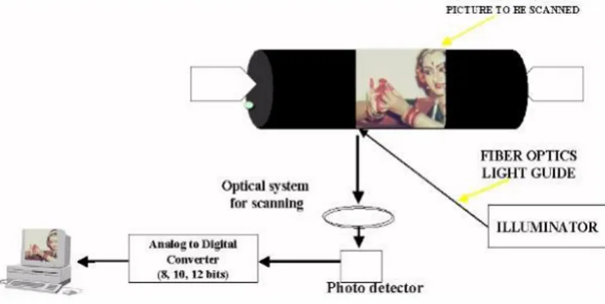
Image Processing (IP) is a mechanism to improve raw images delivered by photographing devices located on satellites, space probes and airplanes or photographs of our daily activists for different uses; different techniques were invented in IP in the past 40-50 years, by using image of divergent source. IP acquired popularity due to its availability of personal computers, memory devices of wide capacity, graphics software, ets. it can be used in divergent application fields of application like remote sensing, medicine photographing, nondestructive evaluation, forensic experiment, textiles, military, cinema industries, document processing, graphic arts and print industry (Gupta and Kaur, 2014). A known stage in the fields of IP are image scrutiny, storing, boosting and translation. Figure (1.1.) is shown a diagram of image scanner-digitizer.
Figure 1.1. Basic Image Processing Technique
Underground of the world cities and roads lie millions of pipes of sewer systems carry away westes, and some of these systems are in a deterioration condition. Maintenance and inspection of defects by human post a major challenge for most of the municipalities. Regular service and defect inspection of the pipelines systems add to life cycle costs and liabilities and in extreme situations causing reduction or even stoppage of services.
Automatic identification of different pipe defects is of substantial importance since it has the potential to solve problems of fatigue, subjectivity, and ambiguity, leading to economic benefits. The main efforts of the research are placed on investigating algorithms and techniques for image pre-processing, segmentation of pipe objects (i.e.,
cracks, holes, joints, laterals, and collapse surface), crack detection, feature extraction and classification of defects.
Pipeline defect detection systems range from simple, visual inspection to complex inspection systems. No one method is universally applicable and operating requirements dictate which method is the most cost effective. Since the last century, efforts were continued to design and construct non-metal sewer pipeline inspection equipment. Many types of equipment have been developed and are being used in developed countries. Among these equipment CCTV, Ultrasound sensor, and Sonar based systems are used. Some of these systems have not become so popular due to the problems of limited practical applications, affordability and acceptability as well as usefulness.
In sixties, using ultrasound sensors invistigetors found many characteristics of these sensors such as object identification by its resonance. Some proposed Smoke Testing technique, this method has been applied in the 1960s for detecting leakage by injection of smoke in the pipe. Whereas, others introduced a technique for location estimation for continuous outdoor translocation of a robot moves autonomously. This technique was based upon maximum similarity calculation. Data combination procedure was also given.
In the 1999s, also, Thermographic non-destructive testing employing thermo-resistance influence of the defect to inspect the most complexed defects inside any complex pipeline system, was introduced. The device has infrared thermal video for measuring the temperature distribution among the surface of the structure. Fiber optical connection system was good method enable to clear vision and find out the wedded part below the robot while moving for inspection, segested in the same years.
But in 2000s, many workers worked on automated image-based inspection, that aims to extract information from an image on the conditions of objects represented in the image. Usually it is impossible to extract this information concerning the dimensions of objects or their defect properties directly from the image. Basically, all machine vision systems involve image acquisition, image pre-processing, segmentation, and extracting relevant features for classification of the type, severity, and extent of defects present in the image.
The old and traditional methods in pipeline inspection were depending upon using inspectors to be sent into the pipe to check and inspect any possible defect occurrence. By this method, the internal situation inside the pipe was efficiently and accurately determined. Hence, this may cause to man dangerous risk and unhealthy environment. In
addition, it is also impractical to be used for some pipeline system. So, new inspection technique has been developed nowadays to deals with this problem, and to substitute the old systems of inspection (Daher, 2015).
The aim of this investigation is to find out accurate and fast detection means of the damages that may occur in the non-metal sewer underground pipelines (i.e. Impurities, Additional aperture, Residues and Capillary fraction (figure 1.2.)). These disorders may be discovered via extracting the characteristic from interior image taken and tackled through suitable filters to improve its appearance and ultimately subjected to feature extraction process to extract and determine their characters, and at last step, finding out and diagnosing the faults and disadvantages may exist in the tested pipelines, through passing the videos into our pre-designed program to get a final report (by ckliking on publish bottun) having all kinds of present defects and time of its occurring in the videos automatically, without the need to the human eye.
a) b)
c) d)
Figure 1.2. Kinds of defects under study a) impurity, b) additional aperture, c) residues and d) capillary fraction
2. LITERATURE REVIEW
Since the beginning of the eighth decade of the last century, efforts were continued to design and construct non-metal sewer pipeline inspection equipment. Many types of equipment have been developed and are being used in developed countries. Among these equipment CCTV, Ultrasound sensor, and sonar based systems are used. Some of these systems have not become so popular due to the problems of limited practical applications, affordability and acceptability as well as usefulness.
2.1 Detect the Leakage
(Magori, 1989) introduced some brilliant ultrasound sensors (some presence detectors) and thermometer Lambda Locked Loop (LLL) flow, and conducted several investigations on these sensors and found many characteristics of these sensors such as object identification by its resonance.
(Allouche and Freure, 2002) proposed Smoke Testing (ST) technique, this method has been applied in the 1960s for detecting leakage by injection of smoke in the pipe. In this method, smoke is injected into the manhole, and after that use a blower to push the smoke through the crack, voids or defects. Leak and defect would be detected when the smoke appears from the pipe segment.
(Feeney et al., 2009) proposed Leak Detectors Technique (LDT), this method is utilized to inspect pipe leakage by diagnosing their noises in pressurized sewer pipe. Its mechanism, however, is estimating the delay in time on the basis of wave speed calculates. Listening rods, underwater microphones, leak noise correlators and in-line devices, are the methods of detecting leakage of pipe.
(Hao et al., 2012) proposed Magnetic Flux Leakage (MFL), in this technique a gauge is inserted into the metallic pipelines. Corrosion can be detected by this method. Also, pitting defects of bad situation can be detected.
(Feng et al., 2016) introduced circumference defects of welding in gas and oil pipes, methods of non-destruction test, and generalized systematic progress in studies on technical principles, the analysis of signals, methods at determine defect size as well as inspection dependability etc. of magnetic flux leakage (MFL) inspection. Also, reported new methods of inspections and gave references for applying of these techniques in defect inspection.
2.2 Image Processing Techniques
(Qin and Bao, 1995) presented Thermographic non-destructive testing (NDT) employing thermo-resistance influence of the defect to inspect the most complexed defects inside any complex pipeline system. The device has infrared thermal video for measuring the temperature distribution among the surface of the structure, a computer with a PIP 1024B image board can conduct image processing for thermographs, as well as a HP inkjet XL printer.
(Duran et al., 2002) reported a detailed method of automatic inspection of defects. This method included many steps starting with segmentation of images into geometrical characters and the location (regions) of the defects. Automatically recognition, assessment, and pipe defects categorization were done by computing of a partial histogram based on adaptive image processing.
(Ohtani and Baba, 2004) introduced a shape recognition system through arrangement of ultrasonic sensor array and CCD image sensors. This technique permits using in cases of difficult to recognize an object shape using ultrasound sensor array alone or CCD image sensor alone.
(Marsland et al., 2005) introduced a substituted method to inspect defects presents in the pipes using novelty detection. A neural network was used to ignore normal conception, that suggested not any problem, therefore, objects that robot did not sense previously was highlighted 18 as a possible error. This decreases the possibility of false negatives. A novelty filter that can be operated on-line was also presented. Hence, every new input was evaluated for novelty regarding the data have been seen.
(Daniels, 2005; Hao et al., 2012) proposed Ground Penetrating Radar (GPR), it is nondestructive technique utilizing electromagnetic waves to detect subsurface materials. Many kinds of GPR are used, such as spatial domain, frequency domain and time domain types. Leak, video, and pipe collapse can be detected by this method.
(Yang and Su, 2008) suggested as a first step using the image processing technique, implicating wavelet transform and computation of co-occurrence matrices, for describing the textures of the pipe defects. Therefore, they adopted three platforms; back-propagation neural network (BPN), radial basis network (RBN) and support vector machine (SVM) to categorize pipe defect format. Results reflected that SVM was the best by given 60% diagnosis accuracy, while Bayesian classifier gave 57.4% diagnosis accuracy.
(Xue-Fei and Hua, 2009) suggested a defect feature extraction algorithm under HSV color space depending upon the image processing. The suggested method able to discover defects from the background, kinds of defects of the underground pipelines could be classified in the estimation steps.
(Gao et al., 2017) proposed an automatic and effective novel methodology for detection and identification the defect in industrial pipelines, is based on image processing. This procedure has three steps. First, conversion the RGB image of the pipelines into a grayscale image. The second is extraction the pipelines and ultimately the detection and identification of the detect.
2.3 CCTV Technique
(Hao et al., 2012) proposed Closed-Circuit Television (CCTV), this technique was first applied in the 1960s for inspection inside the pipelines. In this method, a robot equipped with camera is inserted inside the pipeline from a hole. The robot is controlled by the inspector. By this technique, the inspector can get a lit up image of the defective area from inside of the pipe, does not need the man entry as well as easy to inspect in details by zooming in and out of the area under investigation. On the other hand, some disadvantages are image can only be taken above the water level, image does not contain details about defect dimensions, and it also cannot determine whether a crack extends to the outside surface of the pipe.
(Allouche and Freure, 2002) proposed Sewer Scanner and Evaluation Technology (SSET), this technique was developed to improve CCTV. It is a multi-sensor technique working along the pipe without stopping at every defective area. Therefore, it is more applicable and effective than CCTV. By this method, the test of the defects can be done after the end of the device tour inside the pipeline. This method also, is capable to scan the entire surface of the pipe in 360 degrees, and can inspect horizontal and vertical pipe deflection.
2.4 Laser Technique
(Nassiraei et al., 2007) presented KANTARO, which is the prototype of a passive-active intelligent, completely independent, un-tethered robot with an intelligent unit in its sensor and mode of action. KANTARO, this device has a newly passive-active intelligent mode of action, can move throughout the pipe and passing divergent pipe curvatures easily, without the help of the controller or reading of the sensor. For realizing the
mechanism of the action of this device, a macro-intelligent 2D Laser scanner was developed to detect the navigational landmarks, by the computer and in independent manner. This device has fish eye camera to inspect situation and presented detection.
(Safizadeh and Azizzadeh, 2012) introduced a new methodology depending upon the laser generated rings onto the inner wall of the pipelines. Holes and defects locations on the inner wall of the pipelines are detected via analysis of the intensity of the light. Laser intensity is depending upon many factors, like the ring, angle incidence or smoothness of the scattering surface. Unordinary values in one of these factors may result false defect detection. Therefore, it is necessary to hold an enough knowledge of the laser reflectance phenomena for enhancement of the system performance and for realization of its restrictions.
2.5 Different Other Techniques
(Jensen and Svendsen, 1992) proposed a technique based upon fields of pulse pressure fields from ultrasound transducer. The pulsed pressure fields were estimated by Tupholme Stepanishen method. By this method continuously waved and pulse-resonance can also handle. The calculation of the field was by dividing the surface into small rectangles and then summing their response. By using far-field approximation they got fast estimation of the fields.
(Maeyama et al., 1995) introduced a technique for location estimation for continuous outdoor translocation of a robot moves autonomously. This technique was based upon maximum similarity calculation. Data combination procedure was also given. (Kawaguchi et al., 1995) gave a detailed explanation of a new successful technique, connecting system and vision system of a robot inspecting inside the pipelines, based upon two magnetic wheels. Fiber optical connection system was used for friction reduction. Optical system was made in minimum size, in order to enable it for clear vision and find out the wedded part below the robot while moving for inspection.
(Sinha, 2000) introduces three-steps technique for crack detection, first, D1 and D2 filters were used for extraction the cracks taking into consideration characteristic of pixels in a small vicinity. Secondly, a single respond as well as an associated direction in each pixel. Last stage was the processing of the results by cleaning and relating operations to obtain crack segments.
(Paletta and Pinz, 2000) presented strengthen learning is the context of the detection of the object visually, inclusion of objects identification tasks in corresponding
localization framework. They reported that a decision making learns the efficient fusion behavior directly from the interaction with its stochastic environment in a semiconductor loop. The introduced visual detection system works in adaptive and autonomous manner.
3. MATERIALS AND METHODS
3.1. Materials
Underground sewer systems are used widely for big cities, distract and habituated villages. Municipals always responsible for controlling and managing these systems. This type of business is in general given to privet sector for implementation. After constructing the system, it should be tested and delivered. In case of many defects in the system, the company is responsible for manipulating and fixing the defects and hand the system over. Again the system is submitted to another test by an operator trained for this task.
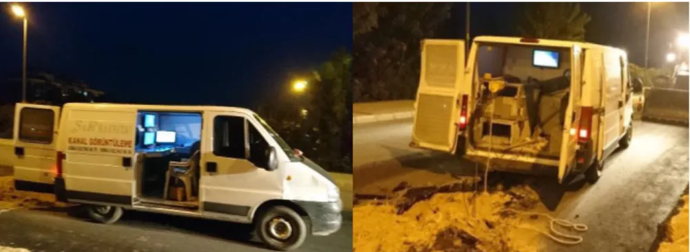
In this study, pipelines are tested and tackled using image processing methods by the images taken from inside the pipelines without the need to the operator. On the other hand, this investigation was conducted on non-metal sewer pipes. Photographing process, however, was done by TENOM YAPI MADENCİLİK, which authorized by the municipals of the Konya city. Figure (3.1.) show the robot having APEX-90 camera used to provide the image required for this study. Figure (3.2.) also imply the detection operation using robot, computer and other tools.
Figure 3.1. Camera and Robot used in photographing inside the pipe
a) b)
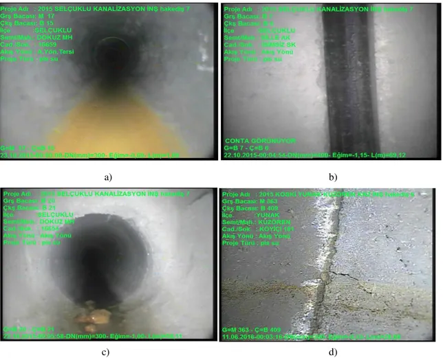
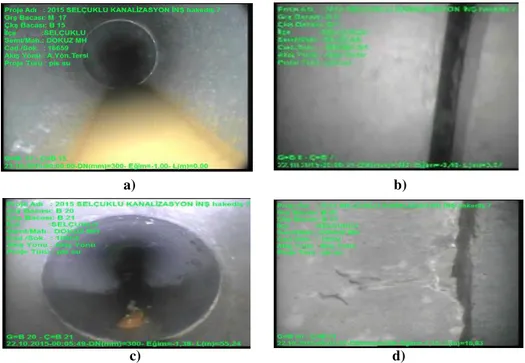
c) d)
Figure 3.3. images (a) Impurity defect, (b) Additional aperture defect, (c) Residues defect and (d) Capillary fraction defect, given by the robot from inside
Figure (3.3. (a, b, c, and d)) shown defects that may occur in the non-metal sewer underground pipelines. These disorders may be discovered by extracting the characteristic from interior image taken from inside the pipes as a videos. These videos have been taken from the company mentioned previously, submitted to predesigned program to convert them into frames (one frame each one second). The frames were categorized into 4 classes (dataset); Impurities (36 images), Additional aperture (33 images), Residues (27 images) and Capillary fraction (23 images). Datasets were classified into classes and used as inputs to detect these defects through extracting their characteristics.
3.2. Methods
3.2.1. Filters
To enhance the images that extracted and classified from the videos, different filters were used. These images passed into filters to eradicate noises that may occur during the process of filming of the video and make them more clearly.
3.2.1.1. Sobel Operator (SO)
In general SO is used in edge detection algorithms to produce image through concentrating on edge and transitions of the image. Irwin Sobel was the inventor of this operator (Sobel, 2014) and named after this inventor. This operator contain two convolution 3*3 matrices (kernels). The first is for estimation gradient -axis (row) and the second estimates -axis slop, which are columns (Othman et al., 2009). This algorithm based on first derivative convolution, analyses derivatives and estimation the gradient of the image intensity at each point, and then it gives the direction to boost the image intensity at each point from light to dark. It plots the edges at the points where the gradient is highest (Poobathy and Chezian, 2014).
Figure 3.4. Sobel convolution Mask
Figure (3.4.) reflects two matrices and , where G is gradient, and represent horizontal and vertical mask axis respectively. These and are integrated to find the gradient at evry point (Poobathy and Chezian, 2014). Then the absolute gradient bulk will be given by equatiıon (3.1):
| | = √ +
(3.1) But often this value is approximated with (Maini and Aggarwal, 2009):| | = | | + | |
(3.2) This operator can smooth the impact of disordered noises in an image. It is differentially isolated by two rows and columns, so the edge parts on both sides become enhanced. This may give bright and thick look of the edges (Maini and Aggarwal, 2009). Figure (3.5.) shows image obtained after applying Sobel filter.a) b)
Figure 3.5. (a) Original image (b) Image Obtained After Applying Sobel Filter
3.2.1.2. Prewitt operator (PO)
It is resembling to Sobel, gradient based operator which compute first derivative. Here ∗ masks are utilized to find out the peak gradient magnitude. When the highest magnitude found, then it works on that direction. Boundaries are detected by the way of either horizontal or vertical manner or both. The figure (3.6.) reflects the 3 x 3 kernels of PO, it uses first derivative to find gradient (Poobathy and Chezian, 2014).
Figure 3.6. Prewitt convolution mask
3.2.1.3. Robert’s cross operator
The simple approximation to gradient magnitude based operator provides ∗ neighborhood of the current pixel. Its convolution masks are,
The figure (3.7.) shows two matrices and , where G is gradient, and are horizontal and vertical mask axis (Poobathy and Chezian, 2014).
3.2.1.4. Canny Operator (CO)
The outstanding algorithm utilizes four major processes to reach virtual edge of a digital image. The four processes are; smoothing, derivation, maxima finding, and thresholding. The first one gives smooth image for conducting the second goal (i.e. derivative of Gaussian); third step is to achieve maxima after derivation. Final process of CO is hysteresis thresholding. The achievement of this Gaussian-based operator is done because of its low error rate and well localization of edge points. Besides, it provides solo boundary. To fulfill this, smoothing is done. Two level thresholding are followed in this way, the weak boundaries are included in the edge map only if it is connected with strong boundary lines (Poobathy and Chezian, 2014).
3.2.1.5. Median Filter (MF)
MF is a non-linear method, used to eradicate noise from images (Mustafa et al., 2012). E.g., salt and pepper noise can be easily minimized by MF. The MF can eradicate noise actively while preserving edges, this is one of its most important features. This is why MF is often used in image segmentation task as we know the importance of the rule played by edges in the process. The procedure of this filter is: it moves through the image pixel by pixel exchanging each value by median value of the nearby pixels (Mittal and Anand, 2013; Bora and Gupta, 2014). The pattern of the neighbors is called the window, which slides, pixel by pixel, over the whole image. The MF is then compute by first sorting all the pixel values from the window into numerical order. Finally, exchange the considering pixel with the median pixel value (Bora et al., 2015).
3.2.2. Algorithms
3.2.2.1. The k-means clustering
The data clustering techniques are important methods to be used by workers dealing with huge databases having data of many variables. On the other hand, it is a method for analyzing data of descriptive nature in order to reveal composition found in the data (Morissette and Chartier, 2013). Data clustering technique is very easy and
applicable method for partition datasets, it aims to yield groups of cases or variables having high level of resemblance in the single group as well as minimum level of resemblance among groups (Hastie et al., 2002).
The major concept of this method is to select center points for each group, the number of each is (K). Center is repeatedly selected in random manner. Each point on the dataset is allocated to its nearest center. This could be repeatedly done until there no longer change in the center points of each group, is exist (Dugad and Desai, 1996; Bilmes, 2006). By this way ideal center points can be produced.
Most of previous research's choose 3 K-means clustering algorithms: - The Forgy/Lloyd algorithm, the MacQueen algorithm and the Hartigan & Wong algorithm. These methods are commonly applied because these techniques almost having slightly different goals and also results. For using any of the above algorithms, in the beginning the number of clusters in the data must be known. This need many tests to find the beast amount of clusters, and data should be standardized as an initiation step in case that ingredients of the cases are not at the same scale. It is well known that there is no absolute best algorithm. The selection of the beast algorithm based on qualities of the datasets regarding size and number of the variables of the case (Morissette and Chartier, 2013). For beast realization of the datasets, many divergent clustering algorithms should be tried (Jain et al., 2000).
3.2.2.1.1. Characteristics of some clustering algorithms:
Lloyd: it is important in its use for sets of huge data, data distribution is distinguished and the optimization of total sum squares. On the other hand, its disadvantages are slowly in the converge process and some empty clusters may be created (Morissette and Chartier, 2013).
Forgy: This algorithm possesses same advantages in Lloyd algorithm except for the data distribution which is here is continuous. As for the disadvantages, they are resembled with that of Lloyd method (Morissette and Chartier, 2013). MacQueen: Initial converge is fast and total sum squares are optimized. Week points in this method are the need to store the two closest-cluster computations for each case, as well as the sensitivity to the system of application of the algorithm to each case (Morissette and Chartier, 2013).
Hartigan: It is fast in initial converge and make the sum of squares within the cluster optimum. This method however having the same weak points of the MacQueen one (Morissette and Chartier, 2013).
3.2.2.1.2. Clustering algorithm
To find out k cluster the main steps of k-means algorithm are (Steinbach et al., 2000): -
Choose k points as primary central points. Allocate all points to the nearest central point. Re-estimate the central point for each cluster.
Apply steps 2 and 3 repeatedly till the stabilization of the central points. An algorithm for partitioning (or clustering) data points into disjoint subsets containing data points so as to minimize the sum-of-squares criterion equation (3.3).
� = ∑− ∑���|��− � |² (3.3)
3.2.2.1.3. Distance metrics
In order to measure the similarity or regularity between the data-items, distance metrics plays a very important role. It is necessary to identify, in what manner the data are interrelated, how various data dissimilar or similar with each other and what measures are considered for their comparison (Singh et al., 2013).
3.2.2.1.3.1. SqEuclidean distance
SqEuclidean distance computes the root of square difference between co-ordinates of pair of objects. The (Euclidean) distance between is found to be Procedure of K-means by equation (3.4) (Singh et al., 2013).
3.2.2.1.3.2. Cityblock distance
Cityblock estimates the distance between and for � times. � is the frequency of estimation. The cityblock distance two point and with � dimensions is defined in equation (3.5) (Bora et al., 2014):
∑ | − |
= (3.5) 3.2.2.1.3.3. Cosine Distance:The cosine distance between two points is one minus the cosine of the included angle between points (treated as vectors). Given an -by- data matrix X, which is treated as m (1-by- ) row vectors , , ..., , the cosine distances between the vector
and are defined as follows equation (3.6) (Bora et al., 2014):
= −
√ − − −(3.6)
3.2.2.2. Feature Extraction (FE)A substantial realm of Artificial intelligence in (FE). It is extraction of the more suitable and interested features of an image and assign it into label. The substantial step in image categorization is the analysis of the image qualities and arrange these results the numerical features into categories. The mean the image categorized on the basis of its content (Morales-González et al., 2014; Seyyedi and Ivanov, 2014).
Categorization model and accuracy rate is depending upon the numerical qualities of different image features that represent the data of the categorization model. Recently many feature extraction technique (FET) were mode up each with its own strong and weak points. A suitable FET is the one which gives relevant features (Qian et al., 2013; Xiao et al., 2013).
3.2.2.2.1. Edge detection (ED)
In order to focus on the edge of an image, it is applicable that few weights of the filter be negative. A first-derivative row filter, at a location in the output image, produces variations in pixel values of the columns on both sides of this site of the input image. So, filters output would be grater (either negative or positive) when there are outstanding
variations in the values of pixel in the right and left sides of the pixel site. A set of weights, which includes some smoothing in averaging over 3 rows is shown by (Moreno et al., 2009; Fu, 2014):
= 6(− − − )
On the contrary second-derivative filters, may be similar and hence, respond to the edges in many orientations, if they remain linear. The arrangement is as follow:
= ( − 8 )
It is same kind of filter that is used to make figure (3.8. (c)), i.e. differences among the output from moving average filter as well as the raw image. With these weights, it can be shown that Laplacian transition of equation (3.7) (Fu, 2014).
∑ =− ∑=− + . + ≈�²�� ² +�²�� ² (3.7)
Result of using of such filter to − image is gives figure (3.8. (a)). Edges manifest the image as zero-crossing in Laplacian that means the Laplacian will be +ve on one side and –ve in the other one. This is because an edge gives max. and min. values in the first derivative and zero value in the second derivative. Figure (3.8. (b)) gives a tool to identify a zero-crossing, and the –ve and +ve values from the first filter shown as black and white respectively. Hence, zero-crossing match to black/white edges. For reducing the impact of the noise to the minimum level, the filter mentioned above or simple version of Laplacian filter is (Fu, 2014):
= ( − )
Figure 3.8. second-derivation filters applied to − image (a) 3*3 Laplacian filter, (b) zero-thresholded version of (a), (c) Laplacian-of-Gaussian filter,σ²=2, (d) zero-thresholded version of (c), (e)
Laplacian of Gaussian filter, σ²=2/3 , (f) zero-thresholded version of (e)
There are three stages of edge detection, pre-processing, feature extraction FE and post-processing. ED process follow is shown figure (3.9.). After pre-processing, of image
I, a middle result I is resulted. This stage emphasizes on noise minimizing and matrix
inhibition, while keeping edges as well as the absence of blurring edges between the divergent fields. The feature extraction has two stages: response computation and feature manipulation. In the first stage, estimation can come from statistical data, and a bunch of features is obtained (Fu, 2014).
Figure 3.9. General edge detection flow
Feature manipulation stage includes, the choose and buildup of feature, so, the result is a bunch of features . The FE stage is the main and necessary stage in edge detection. The aim of FE is to apply them to classify pixels as edge points or non-edge points. After post-processing, a final edge map � is resulted. Post-processing mainly emphasizes many manipulating processes, marking edge points, thinning edges, removing stand-alone edge points and linking broken edge points. Generally, a normal pre-processing technique, such as Gaussian filtering, or a popular post-processing technique, such as thinning operations, can in general cooperate with various FET. This survey mainly covers the stage of extracting features. Most commonly used edge detection algorithms are Sobel, Canny, Prewitt, Roberts, zero-cross & Laplacian of Gaussian (Fu, 2014).
3.2.2.3. Color Features (CF)
Color is the main crucial factor for sorting and recovery of the image, and its curve reflects the (CF) procedure. CF, then, is the allocation of color among the image. Image size, rotation and zoom do not affect the CF, and therefore, here its efficiency lies. (Swain and Ballard, 1991; ping Tian, 2013).
3.2.2.3.1. HSV Color Space
HSV Color area or is uni-color field, HSI (or HSV) means hue ( ), saturation ( ) and intensity ( ) (or value �). Review mentions hue as a color character of light. It could be the character of the surface reflecting or transmitting the light. For insistence, a blue sky gives blue hue. In addition, it is a trait of the human feeling (Acharya and Ray, 2005). Figure (3.10.) shown HSV color space.
Figure 3.10. HSV color wheel
3.2.2.4. Image Segmentation
In image analysis, segmentation is the partitioning of a digital image into multiple regions (sets of pixels), accorded to some homogeneity criterion (Saraf, 2006). The aim of segmentation is to simplify and/or replace the representation of an image into something that is more significate and easier to analyze (Jameel and Manza, 2012).
There are four approach for image segmentation (Saraf, 2006). Threshold techniques.
Edge based methods (Border of object). Region-based techniques.
3.3. Testing of algorithms for defects
To select better algorithm for detecting the defects in our study, each algorithm was applied on 4 defects. The results show that using K-means clustering technique was good enough for detecting of images with Impurities, whereas, for Additional aperture defect, edge detection technique is being the best to identify this type of defects. For image having objects as Residues, color feature (HSV color space) was the best method. Finely as for the Capillary fractions, image segmentation technique gave the best results.
3.3.1. Testing of K-means clustering algorithm Distance measure
That K-means clustering should minimize with respect to type of distance measure for instance:
SqEuclidean: Square Euclidean distance. Cityblock: Some of absolute differences.
Cosine: One minus the cosine of the included angle between points.
Start
Method use to choose initial cluster centroid position such us: Sample: Select K observation from X at random.
Uniform: Select K point uniformly at random from range of X. Matrix: Matrix of starting location.
The distance between the element and the center of the cluster plays an important role in clustering process. Through picking up the suitable measuring mean, better and more accurate results in diagnosing the defect, would be gained. The method of selection starting point of the cluster, is also an important factor in carrying out clustering process. Therefore, K-means clustering technique was examined by selection of many types for distance measuring methods, as well as, many methods of starting center of the cluster. The algorithm was applied on dataset having some defects (i.e. Impurity, Additional aperture, Residues and Capillary fraction). Results are arraigned in the tables (3.1.), (3.2.), (3.3.) and (3.4.) respectively:
Table 3.1. Effect of start point and distance measuring method on accuracy of Impurity detect algorithm using dataset have Impurity defects (%)
Madde Distance
Measurment Method
Sample Uniform Matrix
SqEuclidean 53.1 56.3 100
Cityblock 15.6 31.3 96.9
Cosine 25 25 87.5
Table 3.2. Effect of start point and distance measuring method on accuracy of Impurity detect algorithm using dataset have Additional aperture defects (%)
Madde Distance
Measurment Method
Sample Uniform Matrix
SqEuclidean 8.3 91.7 16.7
Cityblock 16.7 50 8.3
Cosine 8.3 50 25
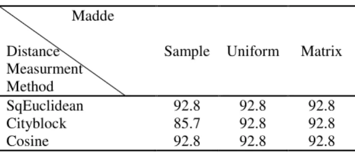
Table 3.3. Effect of start point and distance measuring method on accuracy of Impurity detect algorithm using dataset have Residues defects (%)
Madde Distance
Measurment Method
Sample Uniform Matrix
SqEuclidean 92.8 92.8 92.8
Cityblock 85.7 92.8 92.8
Cosine 92.8 92.8 92.8
Table 3.4. Effect of start point and distance measuring method on accuracy of Impurity detect algorithm using dataset have Capillary fraction defects (%)
Madde Distance
Measurment Method
Sample Uniform Matrix
SqEuclidean 0 60 0
Cityblock 0 40 0
Cosine 20 60 0
It is obvious from the data in the above tables that this algorithm is very applicable for prescribe and identification for any Impurity may present in the pipes.
3.3.2. Testing of edge detection algorithm
To find out the additional aperture algorithm performance and defect diagnosing accuracy, a group of edge detection operator was examined with a group of median filter size. The algorithm was applied on dataset having some defects (i.e. impurity, additional aperture, residues and capillary fraction). Results are arraigned in the tables (3.5.), (3.6.), (3.7.) and (3.8.) respectively:
Table 3.5. Effect of edge detection operator and median mask size on accuracy of Additional aperture detect algorithm using dataset have Impurity defects (%)
Median Mask Size Edge operator [3 3] [5 5] [7 7] [9 9] [11 11] [13 13] Sobel 3.13 6.25 3.13 3.13 3.13 3.13 Canny 0 3.13 3.13 3.13 3.13 3.13 Prewitt 3.13 6.25 3.13 3.13 3.13 3.13 Roberts 0 0 0 0 0 0
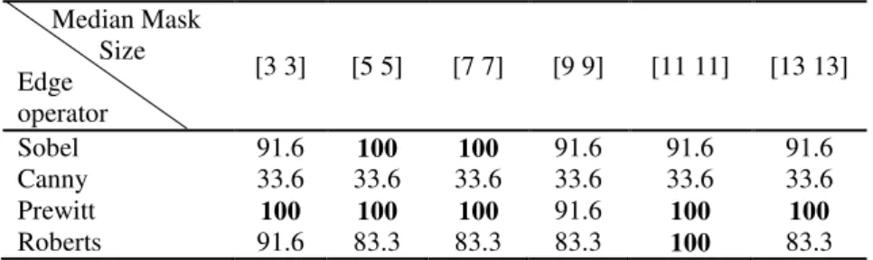
Table 3.6. Effect of edge detection operator and median mask size on accuracy of Additional aperture detect algorithm using dataset have Additional aperture defects (%)
Median Mask Size Edge operator [3 3] [5 5] [7 7] [9 9] [11 11] [13 13] Sobel 91.6 100 100 91.6 91.6 91.6 Canny 33.6 33.6 33.6 33.6 33.6 33.6 Prewitt 100 100 100 91.6 100 100 Roberts 91.6 83.3 83.3 83.3 100 83.3
Table 3.7. Effect of edge detection operator and median mask size on accuracy of Additional aperture detect algorithm using dataset have Residues defects (%)
Median Mask Size Edge operator [3 3] [5 5] [7 7] [9 9] [11 11] [13 13] Sobel 14.29 7.14 14.29 14.29 14.29 7.14 Canny 0 0 14.29 14.29 7.14 14.29 Prewitt 14.29 7.14 14.29 14.29 14.29 7.14 Roberts 7.14 7.14 14.29 7.14 14.29 7.14
Table 3.8. Effect of edge detection operator and median mask size on accuracy of Additional aperture detect algorithm using dataset have Capillary fraction defects (%)
Median Mask Size Edge operator [3 3] [5 5] [7 7] [9 9] [11 11] [13 13] Sobel 60 60 20 20 20 40 Canny 60 60 60 60 60 60 Prewitt 60 60 20 20 20 40 Roberts 40 20 20 40 60 20
It is obvious from the data in the above tables that this algorithm is very applicable for prescribe and identification for any Additional aperture may present in the pipes.
Below tables explain the time required for application of additional aperture. Data in table (3.6.) reflects that 100 % accuracy cases appeared serval times. Therefore, time element was applied to accomplish ideal solution in discovery of additional aperture from the accuracy and time points of view. Table (3.9.) below show the time taken to apply the algorithm:
Table 3.9. Execution time for applying Additional aperture detect algorithm (seconds) Median Mask Size Edge operator [3 3] [5 5] [7 7] [11 11] [13 13] Sobel - 2.34 2.43 - - Prewitt 2.36 2.36 2.40 2.38 2.49 Roberts - - - 2.35 -
3.3.3. Testing of color space algorithm
In applying residues defect discovery, two main factors were manipulated to gain accurate results in defect identification. These factors were saturation elevation and threshold to isolate the high saturation degrees from the processed image. The algorithm was applied on dataset having some defects (i.e. impurity, additional aperture, residues and capillary fraction). Results are arraigned in the tables (3.10.), (3.11.), (3.12.) and (3.13.) respectively:
Table 3.10. Effect of different values of saturation and threshold of segment binary mask on accuracy of Residues detect algorithm using dataset have Impurity defects (%)
Value of saturation Threshold Binary Mask 1.0 1.1 1.2 1.3 1.4 1.5 1.6 1.7 1.8 1.9 2.0 0.1 9.38 9.38 6.25 3.13 3.13 3.13 3.13 3.13 3.13 3.13 3.13 0.2 28.1 28.1 28.88 15.63 12.2 12.5 12.5 12.5 12.5 9.38 9.38 0.3 18.7 6.25 31.95 28.13 28.13 34.38 18.75 25 21.88 18.75 15.63 0.4 12.5 6.25 12.5 18.75 24.24 18.75 31.25 28.1 25 25 28.13 0.5 0 3.13 12.5 9.38 6.25 12.5 25 18.7 28.13 28.13 28.13 0.6 0 0 0 0 6.25 0 0 12.5 18.75 25 18.75 0.7 0 0 0 0 0 0 0 0 0 9.38 12.5 0.8 0 0 0 0 0 0 0 0 0 12.5 12.5
Table 3.11. Effect of different values of saturation and threshold of segment binary mask on accuracy of Residues detect algorithm using dataset have Additional aperture defects (%)
Value of saturation Threshold Binary Mask 1.0 1.1 1.2 1.3 1.4 1.5 1.6 1.7 1.8 1.9 2.0 0.1 8.3 16.7 25 25 25 16.7 16.7 16.7 16.7 8.3 16.7 0.2 8.3 0 0 8.3 16.7 16.7 8.3 8.3 8.3 8.3 8.3 0.3 0 0 0 0 0 8.3 0 0 0 0 0 0.4 0 0 0 0 0 0 0 0 0 0 0 0.5 0 0 0 0 0 0 0 0 0 0 0 0.6 0 0 0 0 0 0 0 0 0 0 0 0.7 0 0 0 0 0 0 0 0 0 0 0 0.8 0 0 0 0 0 0 0 0 0 0 0
Table 3.12. Effect of different values of saturation and threshold of segment binary mask on accuracy of Residues detect algorithm using dataset have Residues defects (%)
Value of saturation Threshold Binary Mask 1.0 1.1 1.2 1.3 1.4 1.5 1.6 1.7 1.8 1.9 2.0 0.1 14.3 92.8 7.1 7.1 7.1 0 0 0 0 0 0 0.2 50 50 42.9 35.7 35.7 35.7 28.6 28.6 28.6 28.6 14.3 0.3 87.6 100 85.7 57.1 57.1 50 50 42.9 42.9 35.7 35.7 0.4 57.1 57.4 57.1 78.6 78.6 100 85.7 64.3 57.1 57.1 50 0.5 14.3 28.5 50 35.7 42.9 57.1 57.1 92.9 92.9 92.9 85.7 0.6 0 7.1 14.3 28.6 42.9 57.1 50 50 57.1 57.1 78.6 0.7 0 0 0 7.1 14.3 14.3 28.6 50 57.1 57.1 50 0.8 0 0 0 0 0 0 14.3 21.4 35.7 42.9 57.1
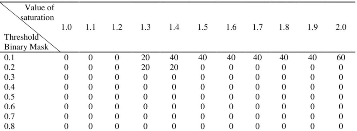
Table 3.13. Effect of different values of saturation and threshold of segment binary mask on accuracy of Residues detect algorithm using dataset have Capillary fraction defects (%)
Value of saturation Threshold Binary Mask 1.0 1.1 1.2 1.3 1.4 1.5 1.6 1.7 1.8 1.9 2.0 0.1 0 0 0 20 40 40 40 40 40 40 60 0.2 0 0 0 20 20 0 0 0 0 0 0 0.3 0 0 0 0 0 0 0 0 0 0 0 0.4 0 0 0 0 0 0 0 0 0 0 0 0.5 0 0 0 0 0 0 0 0 0 0 0 0.6 0 0 0 0 0 0 0 0 0 0 0 0.7 0 0 0 0 0 0 0 0 0 0 0 0.8 0 0 0 0 0 0 0 0 0 0 0
It is obvious from the data in the above tables that this algorithm is very applicable for prescribe and identification for any Residues may present in the pipes.
Below tables explain the time required for application of Residues algorithm. Data in table (3.12.) also reflects that 100 % accuracy cases appeared more than one time. So, it was successful to exploit the time element once again to achieve the proper solutions to discover the residues as accurate and swift as possible. Below the time required for application of this algorithm presented in table (3.14.):
Table 3.14. Execution time for applying Residues detect algorithm (seconds) Value of saturation Threshold Binary mask 1.1 1.5 0.3 4.44 - 0.4 - 4.48
3.3.4. Testing of image segmentation algorithm
An important two factors with applying capillary fraction identification algorithm, are obviously impact the efficiency and accuracy of the used algorithm. The first is the operator type used in edge detection technique, whereas, the second is, also, the threshold factor. In this realm, divergent types of operators, and many levels of threshold factor were selected to carry out this study. The algorithm was applied on dataset having some defects (i.e. impurity, additional aperture, residues and capillary fraction). Results are arraigned in the tables (3.15.), (3.16.), (3.17.) and (3.18.) respectively:
Table 3.15. Effect of edge operator and threshold factor on accuracy of Capillary fraction detect algorithm using dataset have Impurity defect (%)
Threshold factor Edge operator 0.1 0.2 0.3 0.4 0.5 0.6 0.7 0.8 0.9 1.0 1.1 1.2 Sobel 0 0 0 0 0 3.13 6.25 12.50 6.25 6.25 0 0 Canny 0 0 0 0 0 0 0 0 0 0 0 0 Prewitt 0 0 0 0 0 3.13 0 6.25 12.50 0 0 0 Roberts 0 0 0 0 0 3.13 0 9.37 9.37 3.13 0 0
Table 3.16. Effect of edge operator and threshold factor on accuracy of Capillary fraction detect algorithm using dataset have Additional aperture defect (%)
Threshold factor Edge operator 0.1 0.2 0.3 0.4 0.5 0.6 0.7 0.8 0.9 1.0 1.1 1.2 Sobel 0 0 8.3 8.3 16.7 33.3 8.3 0 16.6 25 25 8.3 Canny 0 0 0 0 0 0 0 0 0 0 0 0 Prewitt 0 0 8.3 8.3 33.3 16.6 8.3 16.6 8.3 25 25 0 Roberts 0 0 8.3 25 25 16.6 16.6 0 0 16.6 25 25
Table 3.17. Effect of edge operator and threshold factor on accuracy of Capillary fraction detect algorithm using dataset have Residues defect (%)
Threshold factor Edge operator 0.1 0.2 0.3 0.4 0.5 0.6 0.7 0.8 0.9 1.0 1.1 1.2 Sobel 0 0 0 0 0 0 0 0 0 0 0 0 Canny 0 0 0 0 0 0 0 0 0 0 0 0 Prewitt 0 0 0 0 0 0 0 0 0 0 0 0 Roberts 0 0 0 0 0 0 0 0 0 0 0 0
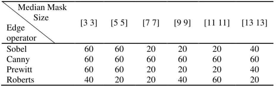
Table 3.18. Effect of edge operator and threshold factor on accuracy of Capillary fraction detect algorithm using dataset have Capillary fraction defect (%)
Threshold factor Edge operator 0.1 0.2 0.3 0.4 0.5 0.6 0.7 0.8 0.9 1.0 1.1 1.2 Sobel 0 0 20 0 40 60 40 60 100 40 0 0 Canny 0 0 0 0 0 0 0 0 0 0 0 0 Prewitt 0 0 0 0 40 60 40 60 60 40 0 0 Roberts 0 0 0 0 40 40 40 40 60 60 40 0
It is obvious from the data in the above tables that this algorithm is very applicable for prescribe and identification for any Capillary fraction may present in the pipes.
3.4. Implementation of algorithms
3.4.1. Implementation of K-means clustering algorithm
The locations of the impurities in the images contained them, are slightly differ in color from the other parts of the image. This is an important character for the image including this type of defects. This trait was used in this investigation to detect impurities present in the input images as shown in figure (3.11.), by employing K-means clustering technique.
Figure 3.11. Image contained impurity
This technique is the most common algorithm used in data analysis due to its simplicity and distinguished mathematical performance, based it can be applied to evaluate datasets on the bases of clustering them into 2-clusters, one of them contains similar characteristics represent the impurities that are the important part to be gained, regardless the other data of the image. That is why the selection was classified them into cluster (i.e. no. of clusters = 2). Similitude scale (Euclidian distance) was employed in this study. This scale, however, plays an important role in classification and finding out datasets, depending upon the similitude of these data and ultimately finding the center point for each group.
The classification output was index 1 and 2, where (1) represent the first cluster, whereas (2) is the second one as shown in figure (3.12.).
Figure 3.12. Output image indexed by 0 and 1
The index was converted into image, in this image the pixels with 255 value is the impurities, and pixels with 0 value is the other data in the original image, figure (3.13.) illustrate the output image.
Figure 3.13. Image results by converting index
Finally, in this trial it was found that the object was the impurities, and by estimates and study its characters (area, length, and width) as measurement units, it was possible to distinguish the image having this type of defects from the other image of datasets.
Image analysis as well as finding the number of objects in the image helped in understanding and manifestation of image contents and finally make a suitable decision whether these images contain impurities. Image with object = 0 is free of impurities and the vice is not always versa. The image with impurities could analysis and the information may be extracted by estimating the area of the object which is sum of pixels within the object that can be used as measurement unit. Here, in the image containing impurities as a defect, the object area would be greater as compared to that free of this defect.
No
Yes Read image
Convert image from RGB into L*a*b color space
Reshape the L*a*b image
Insert the number of color which will cluster
Apply k-means clustering with SqEuclidean for distance measure,
and Matrix for start point
Cropped the image
Convert index into image
Apply Morphological image open
Convert the image into binary
image
Calculate and labeled the area and number of objects
IF The Number of object > 0 There is No Impurity
No
Yes
Flowchart 1 Impurity detection algorithm
The code of impurities algorithm
function z = Mildet( im ) he=im; rect=[0 40 630 570]; I2 = imcrop(he,rect); A=I2(1:180,:,:); B=I2(180+1:end,:,:); B1=imcrop(B,[11 0 630 300]); [m n k]=size(B1);
cform = makecform('srgb2lab'); lab_he = applysform(B1,cform); ab = double(lab_he(:,:,2:3)); nrows = size(ab,1);
Calculate number of objects (No), area and number of hole
(HW) IF No > 5 | Area < 6000 | HN > 5 There is No Impurity There is Impurity
ncols = size(ab,2);
ab = reshape(ab,nrows*ncols,2); C=[m 55; m 54;m 22];
Seed = [1 1; 270 260]; nColors =2;
[cluster_idx] = kmeans1(ab,nColors,'distance','sqEuclidean', 'Start',Seed); pixel_lapels = reshape(cluster_idx,nrows,ncols); I=pixel_labels; [m n] =size(I); for i=1:m for j=1:n if I(i, j)==1 p(i, j)=0; else p(i, j)=255; end end end se = strel('disk',7); p = imopen(p,se); level=graythresh(p); bw=im2bw(p,level); [labeled,numObjects]=bwlabel(bw,4); info=regionprops(labeled,'all'); if(numObjects>0) info(1).Area; Areas=cat(1,info.Area); mask=logical(p); red=immultiply(mask,B1(:,:,1)); g=immultiply(mask,B1(:,:,2)); b=immultiply(mask,B1(:,:,3));
im=cat(3,red,g,b); [m n k]=size(im); I=reshape(im,m*n,3); idx=find(mask); level=graythresh(p); bw=im2bw(p,level); [labeled,numObjects]=bwlabel(bw,4); info=regionprops(labeled,'all'); Euler_Number1=info(1).EulerNumber; NumHoles1=1-Euler_Number1; bigest_Area=info(1).Area; l=1; for i=2:numObjects if(bigest_Area<info(i).Area) bigest_Area=info(i).Area; l=i; end end in=find(cat(1,info.Area)==bigest_Area); [m n K]=size(B1); No=numObjects; HN=NumHoles1 ; area=bigest_Area; if ( area < 7140 )
disp ('there are No impurities'); z=0;
else
disp ('there are impurities'); z=1;
end else
disp ('here no impurities'); z=0;
end end
3.4.2 Implementation of edge detection algorithm
Image with additional apertures (aperture of the joint between pipes) are characterized with discontinuity or sudden change in some optical properties such as, light intensity, structure or color. Therefore, for such image with these defects, edge detection technique was applied as shown down in figure (3.14.).
Figure 3.14. Additional aperture image
The basic concept of this technique is that, the edge information could be found through the relationship between each pixel in the image with the surrounding pixels. Edges in this types of image comprise specific useful information for image analysis and detect the additional apertures as well. Sobel operator with threshold equal to 0.020 was followed to detect the image edge. The function of this technique was to lineation of the objects of the image (i.e. additional apertures) by boosting the image brightness, eliminating many un-useful information in image analysis process. After applying the technique, bi-sector image with additional apertures boarders was obtained, in addition to presence of some edges inside and outside the apertures boarders as noise as shown in figure (3.15.)bellow.
Figure 3.15. Applying Sobel with threshold 0.020
The next step was the elimination of the noise inside and outside the object (apertures). By image close morphological technique, that is dilation followed by erosion. So, the result was logical image of background which is (0) value and additional apertures which have the value (1) for the pixels, figure (3.16.) bellow illustrate the output logical image.
Finally, the properties of the object (apertures) were used as measurement units for measure and comparison to detect the image having additional apertures as defect.
Figure 3.16. The output logical image.
This line was analyzed and its properties were extracted and used for distinguish the image containing such type of defects from the other images. For instance, the length of the object was measured and used to verify whether object additional aperture or not. Length was used for further analysis, if it is less two-thirds of the image length so, this object is not additional aperture. On the other hand, object width has an importance not less than the importance of the length quality. Width has also been measured and used to