Contents lists available atScienceDirect
Applied Energy
journal homepage:www.elsevier.com/locate/apenergy
Bene
fits of transmission switching and energy storage in power systems with
high renewable energy penetration
Meltem Peker, Ayse Selin Kocaman
⁎, Bahar Y. Kara
Department of Industrial Engineering, Bilkent University, 06800 Ankara, TurkeyH I G H L I G H T S
•
A stochastic programming approach is proposed to model TS and ESS sizing simultaneously.•
The model considers DSM and renewable energy curtailment policies with various limits.•
The effect of TS on total cost, sizes, locations of ESS are discussed.•
Wefind that TS is noteworthy to analyze for power systems with renewable targets. A R T I C L E I N F OKeywords:
Transmission switching Renewable energy Energy storage siting Energy storage sizing
A B S T R A C T
Increasing the share of renewable energy sources in electricity generation helps address concerns about carbon emissions, global warming and energy security (i.e. dependence on fossil fuels). However, integrating inter-mittent and variable energy sources into the grid imposes new challenges for power system reliability and stability. To use these clean sources in electricity generation without endangering power systems, utilities can implement various control mechanisms, such as energy storage systems, demand side management, renewable energy curtailment and transmission switching. This paper introduces a two-stage stochastic programming model that co-optimizes transmission switching operations, and transmission and storage investments subject to limitations on load shedding and curtailment amounts. We discuss the effect of transmission switching on the total investment and operational costs, siting and sizing decisions of energy storage systems, and load shedding and renewable energy curtailment in a power system with high renewable penetration. An extensive compu-tational study on the IEEE 24-bus power system with wind and solar as available renewable sources demon-strates that the total cost and total capacity of energy storage systems can be decreased up to 17% and 50%, respectively, when transmission switching is incorporated into the power system.
1. Introduction 1.1. Motivation
In the last two decades, the electricity industry experienced major changes. Increasing concerns about the environment and energy se-curity reveal the necessity of using clean and sustainable energy re-sources in electricity generation. To encourage new investments to use more renewable energy sources (RESes), utilities implement policies such as feed-in tariffs, carbon taxes and/or renewable portfolio stan-dards [1], and as a result, a 19% share of RESes in meeting world electricity demand in 2000 increased to 24% in 2016[2]. Improve-ments such as this help reduce carbon emissions and dependence on fossil fuels. However, increased penetration of RESes can lead to high
variability and uncertainty in electricity generation as these sources are intermittent and dependent on atmospheric conditions and spatial lo-cations. Low predictability and variability of electricity generation from RESes can cause difficulties in sustaining a load-energy balance and/or power frequency in a grid, and thus can impose new challenges around power system reliability and stability. To continue utilizing these clean sources without endangering power system reliability, utilities imple-ment various control mechanisms such as energy storage systems (ESSes), demand-side management (DSM), renewable energy curtail-ment (REC) and transmission switching (TS).
Energy storage systems are the most effective solutions for in-tegrating RESes into the grid. These systems smooth the intermittency of RESes by storing electrical energy generated at off-peak hours to use at peak hours, and thus more electricity can be generated from RESes
https://doi.org/10.1016/j.apenergy.2018.07.008
Received 4 April 2018; Received in revised form 12 June 2018; Accepted 1 July 2018 ⁎Corresponding author.
E-mail address:[email protected](A.S. Kocaman).
Available online 08 July 2018
0306-2619/ © 2018 Elsevier Ltd. All rights reserved.
and a substantial decrease in greenhouse gas emissions can be achieved. Demand-side management is another control mechanism that helps utilities reduce demand at peak hours (referred to as load shedding (LS) in this paper) or reshape load profiles[3]. Efficient DSM can also reduce the need for peaking power plants and/or under-utilized electrical in-frastructures, which can have high investment and operational costs. However, reducing demand at peak hours intentionally affects quality of life. Therefore, a penalty cost (value of loss load) is generally con-sidered to compensate for the impact of cutting electricity[4].
Renewable energy curtailment is also used to handle RES varia-bility. With an increase in RES penetration, a significant amount of renewable energy could be curtailed due to technical and operational reasons to maintain system voltage and frequency levels or to satisfy minimum generation requirements from thermal sources[5]. However, by lowering RES supply, the benefits of using clean sources and rev-enues from renewable generators are reduced. Thus, to promote new investments in sustainable energy, in some markets, revenue losses from renewable energy generators are sometimes compensated for in some contracts/policies[6,7].
Transmission switching is another control mechanism that adds flexibility to the grid. Transmission congestion, which is another reason for low RES shares in electricity generation, can be prevented by changing the status of transmission lines [8]. Thus, by applying TS operations (switching some lines out of service), RES penetration can be easily increased. Reducing congestion on transmission lines may also improve the efficiency of other components (e.g. generation units) or other control mechanisms, such as ESS, LS and REC. Making optimal siting and sizing decisions for ESS by considering TS operations can decrease the total investment cost of ESS. In addition, efficient DSM policies can be applied with the integration of TS, and thus LS, which is due to transmission congestion, can be minimized. Last but not least, as REC can be a significant waste, especially for countries that have re-newable energy targets (such as Australia, Turkey, Brazil and Ireland [9,10]), TS can be a more efficient and cheaper solution compared to building new lines or more expensive ESSes. Therefore, considering TS
in power system strategic and/or operational planning leads to higher social welfare by decreasing overall costs, enhancing quality of life and utilizing cleaner sources in electricity generation.
1.2. Literature review
Energy storage systems are effective solutions to the need for cleaner energy sources in electricity generation[4]. The value of ESSes has been increasingly discussed in the literature from different per-spectives. Most studies focus on system operation and determine the ESS’ state of charge (SOC) for each time period[11]. In these studies, given the locations and sizes of the storage units, the aim is to maximize profit by bidding/selling operations in energy markets. However, these studies ignore the effect of ESS locations and sizes (e.g.[12]). To ad-dress this deficiency, other studies consider ESS locations and opera-tions simultaneously for multi-stage[13], robust[14]and long-term [15]planning problems. There are also a few studies that optimize only ESS sizes under demand and generation uncertainties[16].
To fully reveal the benefits of ESSes, their siting and sizing decisions should be considered simultaneously during the planning stage; how-ever, few papers focus on this co-optimization. Pandžić et al. [11] propose a three-stage heuristic algorithm to solve the co-optimized problem. Wogrin and Gayme [17] analyze ESS sizes for different technology types, such as pumped storage hydro, compressed-air en-ergy storage, lithium ion batteries andfly-wheel energy storage, and conclude that the ESS sizes and locations are affected by technology type. Fernáandez-Blanco et al.[18]examine the effect of REC penalty costs and the capital costs of storage units on optimal ESS locations and sizes. Go et al.[19]assess the value of co-optimizing ESS, generation and transmission expansion planning on the IEEE 24-bus power system. They consider renewable portfolio standards and require a minimum generation from renewable sources. Xiong and Singh[20] limit the budget of ESS investments and discuss the effect of budget on ESS lo-cations. Qiu et al.[21]focus on long-term planning and minimize total system cost considering battery lifetime and degradation.
Nomenclature
Sets
B set of buses, indexed by i j,
C (CR) set of all (renewable) generation units, indexed by g A (EA) set of all (existing) lines, indexed by a
ASij set of lines between buses i and j T set of hours of a scenario, indexed by t S set of scenarios, indexed by s
+a
Ψ ( )(Ψ ( )−a) sending-end (receiving-end) bus of line a
Parameters
Dits demand of bus i at hour t of scenario s (MW)
Gigts, (Gigts) maximum (minimum) generation limits from unit g in bus i at hour t of scenario s (MW)
Rgup(Rgdown) ramp-up (ramp-down) rate of unit g cgom operation cost of unit g ($/MWh)
Fa capacity of line a (MW)
caline annualized investment cost of candidate line a ($)
φa susceptance of line a (p.u.)
E, (E) maximum (minimum) energy capacity of energy storage systems (ESS) (MWh)
P, (P) maximum (minimum) power rating of ESS (MW)
cE annualized investment cost of ESS for energy capacity ($/MWh)
cP annualized investment cost of ESS for power rating
($/MW)
cd discharging (or ageing) cost of ESS ($/MW) η charging/discharging efficiency of ESS
α energy-power ratio of ESS
E0 initial energy level of ESS
σs probability of scenario s
NS number of days in the target year
τ maximum number of switchable lines
pls ratio of load that can be shed to total load
prec ratio of renewable generation that can be curtailed to total generation
Decision variables
La 1 if candidate line a is built, 0 o.w.
Yi 1 if ESS is built at bus i, 0 o.w. YiE energy capacity of ESS at bus i
YiP power rating of ESS at bus i
Pitsc charging rate of ESS at bus i at hour t of scenario s
Pitsd discharging rate of ESS at bus i at hour t of scenario s
Xits status of ESS at bus i at hour t of scenario s, 1 is for charging/0 is for discharging
Eits state of charge of ESS at bus i at hour t of scenario s Gigts power generation of unit g in bus i at hour t of scenario s DSits load shedding amount at bus i at hour t of scenario s
fats powerflow on line a at hour t of scenario s
Zats 1 if line a is closed at hour t of scenario s, 0 if it is open
The benefits of TS are discussed in many studies from perspectives such as reliability [22,23], economic efficiency [24]and expansion planning[25]. The beneficial impacts of TS on real-world examples are also discussed in[26]for the California and New England independent system operators (ISOs), and in[27,28]for the PJM system. However, only a few papers discuss the effect of TS on RES penetration. Villumsen et al.[29]analyze the effect of TS on wind power penetration levels and line capacity expansion plans. Qiu and Wang[30]discuss the effect of TS on total system cost and utilization of wind power, considering the uncertainty of wind power generation. Nikoobakht et al.[31]develop a linearized AC model to analyze TS operations and RES utilization. However, none of these studies includes ESSes. To the best of our knowledge, only a few papers simultaneously consider TS operations and ESS investment planning. Nikoobakht et al.[32]and Aghaei et al. [33]optimize TS and storage operations in a unit commitment problem without allowing new investments. Dehghan and Amjady[34]discuss an investment planning problem and determine the locations of new transmission lines and storages. However, these studies do not consider ESS sizing decisions.
InTable 1, we compare our study with the existing literature; except for our study, there is no paper that co-optimizes TS operations, transmission and ESS investments (i.e. ESS locations and sizes). A vertically integrated utility where a central planner makes all invest-ment and operation decisions can benefit from this co-optimization process, as planning for TS operations can potentially provide a cheaper solution for countries with renewable energy targets. As presented in Table 1, most studies include penalty costs for LS and/or REC policies to compensate for their impacts on quality of life and revenue losses from renewable energy generators. However, we note that operational and/ or tactical plans may be affected if these penalty costs are not well defined. Moreover, the impact of the cost parameters might be more prominent if both are considered in the planning phase, as used in this paper. Therefore, instead of using monetary values for LS and REC, we limit LS and REC amounts and examine the effects of these limits on the solutions.
1.3. Contribution of the paper
This paperfills a gap in the literature by simultaneously considering TS, ESS siting and sizing decisions, and examining the effect of TS on the other control mechanisms, such as ESS, LS and REC. In this
direction, we propose a two-stage stochastic programming model that co-optimizes TS operations, transmission and storage investments. We then discuss the effect of TS on total system cost, ESS locations and sizes, LS and REC on the IEEE 24-bus power system. Using these ana-lyses, we precisely characterize the joint benefits of TS and ESSes, and show that total cost and total storage capacity can be decreased up to 17% and 50%, respectively, when TS operations are incorporated into the power system. Therefore, TS, which is less costly than building new lines or ESSes, should be considered as an efficient solution, especially for power systems with high renewable energy targets.
In this paper, instead of using penalty costs to compensate for the impacts of LS and REC, the model limits LS and REC amounts. The results obtained with different limits provide insights about the role of storage units for LS and REC control mechanisms. Wefind that ESSes are very effective system component in meeting the various REC limits. However, the role of storage units is limited to tight LS restrictions (cases where a high portion of demand must be met), and thus the effect of TS on this role of storage units becomes more prominent as the limits on REC and LS are relaxed.
The paper continues as follows: In Section2, we explain the problem and provide the proposed mathematical model. In Section3, we present the results of our extensive computational study and examine solutions around the value of TS. We conclude with somefinal remarks in Section 4.
2. Mathematical model
In this section, we introduce our model, which jointly optimizes new investments and operational decisions. As the aim of this paper is to present the joint benefit of ESSes and TS, we assume that planning is done by a vertically integrated utility. For accurate representation of storage units, we consider both energy capacity and power ratings (ramp rates for charging/discharging) of ESSes. In our model, we ignore the cost for generating electricity from available RESes, as customarily done in the literature. For the sake of computational tractability, a static planning approach and a DC approximation of powerflow con-straints, as given in[35], are used in the proposed model, as also used in[15,19,34].
2.1. Mathematical formulation
In this section, we provide an extensive form of a two-stage sto-chastic programming model for the problem. The decisions made in the first stage include investments of transmission lines and ESSes. The second stage involves recourse actions that are based on operational decisions such as powerflows, generation amounts and transmission line status (open/closed) at each hour of the representative days. Each representative day is considered as a scenario with probability σs, which is proportional to the occurrence of similar days based on random ob-servations in the target year.
The objective function minimizes the total investment costs of new transmission lines (zline) and storage units (zstorage), as well as the ex-pected operational costs of conventional generators and ESSes (zom). The objective function is presented below and subject to the following constraints:
+ +
min zline zstorage zom (1)
= ∑ = ∑ + = ∑ ∑ ∑ ⎧ ⎨ ⎩ ∑ + ⎫ ⎬ ⎭ ∈ ∈ ∈ ∈ ∈ ∈ ⧹ z c L z c Y c Y z NSσ c G c P ( ) line a A EA a line a storage i B E iE P iP om s S s i B t T g C C gom igts d itsd \ R
•
Power Balance Constraint: Table 1Comparison of the literature and the current study.
Investment Pen. cost Pen. cost ESS TS costs for LS for REC sizing Villumsen et al.[29] line
Pandžić et al.[11] ESS Li and Hedman[12]
Hedayati et al.[13] line, ESS Conejo et al.[15] line, ESS Jabr et al.[14] line, ESS Wogrin and Gayme
[17]
ESS Fernández-Blanco et al.
[18]
ESS Go et al.[19] gen., line, ESS Xiong and Singh[20] ESS Qiu et al.[21] line, ESS Qiu and Wang[30]
Nikoobakht et al.[31]
Nikoobakht et al.[32]
Aghaei et al.[33]
Dehghan and Amjady
[34]
line, ESS
Our study line, ESS
∑
+∑
−∑
− + = − ∀ ∈ ∈ ∈ ∈ ∈ − = ∈ + = G f f P P D DS i B t, T s, S g C igts a A a i ats a A a iats itsc itsd its its
Ψ ( ) Ψ ( )
(2) Constraint(2)guarantees the power balance at node i at each time period, which includes generation from both conventional and re-newable sources, incoming/outgoingflows, ESS charging and dis-charging rates and demand and load shedding amounts.
•
Generation Dispatch Constraints:⩽ ∀ ∈ ∈ ∈ ∈
Gigts Gigts i B, g CR, t T, s S (3)
⩽ ⩽ ∀ ∈ ∈ ∈ ∈
Gigts Gigts Gigts i B, g C C\ R, t T, s S (4)
⩽ − ⩽ ∀ ∈ ∈ ∈ ∈
Rgdown G G R i B, g C C\ , t T, s S
igts igt s-1 gup R (5)
Constraints(3) and (4) set lower and upper bounds for electricity generation from renewable and conventional sources, respectively. Constraint(5)limits the maximum allowable change of generation from conventional sources between consecutive time periods.
•
Network Constraints:−F Za ats⩽fats⩽F Za ats ∀a∈A, t∈T, s∈S (6)
= − ∀ ∈ ∈ ∈
fats φ Za ats(θits θjts) a ASij, t T, s S (7)
⩽ ∀ ∈ ∈ ∈ Zats La a A, t T, s S (8)
∑
⩽∑
+ ∀ ∈ ∈ ∈ ∈ L Z τ t T, s S a A a a A ats (9) Constraint(6)limits theflow on the closed lines and also enforces that there is noflow on the open lines[34]. Constraint(7)defines the powerflow on the closed lines as a function of the buses’ voltage angles, considering a DC approximation of powerflow constraint. The constraint also guarantees that there cannot be anyflow on lines that are switched off. Constraint(8)satisfies that a line is built if it is used (or closed) [34] and Constraint (9) limits the number of switchable lines withτ.•
ESS Constraints: ⎜ ⎟ = + ⎛ ⎝ − ⎞ ⎠ ∀ ∈ ∈ ∈ E E t ηP ηP i B t T s S Δ 1 , ,its it s-1 itsc itsd
(10) ⩽ ⩽ ∀ ∈ ∈ ∈ EYi Eits YiE i B, t T, s S (11) ⩽ ⩽ ∀ ∈ ∈ ∈ EYi YiE E Yi i B, t T, s S (12) ⩽ ⩽ ∀ ∈ ∈ ∈ PYi YiP P Yi i B, t T, s S (13) ⩽ ∀ ∈ ∈ ∈ Pitsc YiP i B, t T, s S (14) ⩽ ∀ ∈ ∈ ∈ Pitsd Y i B, t T, s S iP (15) ⩽ ∀ ∈ ∈ ∈ Pitsc P Xits i B, t T, s S (16) ⩽ − ∀ ∈ ∈ ∈ Pitsd P(1 Xits) i B, t T, s S (17) ⩽ ∀ ∈ ∈ ∈ αYiP YiE i B, t T, s S (18) = = ∀ ∈ ∈ Ei s0 EiTs E Y0 i i B, s S (19)
Constraint(10) satisfies the energy balance between consecutive time periods. Constraint(11)limits storage units SOC levels by their capacities, and Constraint(12) guarantees that storage capacity is between the predetermined lower and upper bounds. Constraint (13) also sets lower and upper bounds for storage units’ power ratings. Constraints(14) and (15)are the ramp rate of the storage units and limit their charging and discharging rates by their power ratings. Constraints (16) and (17) prevent ESSes from simulta-neously charging and discharging[19]. Constraint(18)relates en-ergy capacity and power rating via a given ratio. A daily storage cycling constraint(19)is added to enforce the storage energy bal-ance for each representative day, as in[15,17,19].
•
LS and REC Constraints:∑ ∑
⩽∑ ∑
∀ ∈ ∈ ∈ ∈ ∈ DS p D s S i B t T its ls i B t T its (20)∑ ∑ ∑
⩾ −∑ ∑ ∑
∀ ∈ ∈ ∈ ∈ ∈ ∈ ∈ G (1 p ) G s S i B g C t T igts rec i B g C t T igts R R (21)As explained earlier, instead of using monetary values for LS and REC, we limit their amounts. Constraints(20) and (21)set upper bounds for the LS and REC amounts, respectively.
•
Domain Constraints: = ∀ ∈ La 1 a EA (22) = ∀ ∈ ∈ θref ts, 0 t T, s S (23) − ⩽π θits⩽π ∀ ∈i B, t∈T, s∈S (24) ⩾ ∀ ∈ ∈ ∈ ∈Gigts 0, θ ursits i B, g C, t T, s S (25)
⩾ ⩾ ⩾ ⩾ ⩾ ∀ ∈ ∈ ∈ P P X E DS i B t T s S 0, 0, 0, 0, 0 , ,
itsd itsc its its its
(26)
∈ ∈ ∀ ∈ ∈ ∈
La {0, 1}, fatsurs, Zats {0, 1} a A, t T, s S (27)
∈ ⩾ ⩾ ∈
Yi {0, 1}, YiE 0, YiP 0 i B (28)
Constraints(22)–(28)are for the domain restrictions of the decision variables. Constraint(22)is for the existing lines and Constraint(23) is the reference point for the buses’ voltage angles. The remaining constraints are the nonnegativity and binary constraints for the decision variables.
2.2. Linearization of the model
We note that the model is nonlinear due to the multiplication of decision variables in Constraint(7). Here, we linearize the model by utilizing the Big-M type of linearization technique. Two nonnegative flow variables,f+
atsand
−
fats, each one representingflow on the same line in one direction, expressfatsas follows:
= +−− ∀ ∈ ∈ ∈
fats fats fats a A, t T, s S (29)
Similarly, two nonnegative variables,Δθ+
atsandΔθats, express the voltage− angle difference between buses i and j as follows:
− = +− − ∀ ∈ ∈ ∈
θits θjts Δθats Δθats a ASij, t T, s S (30)
By using(29) and (30), Constraint (7)is linearized and replaced with the following constraints:
⩽ ∀ ∈ ∈ ∈ + + fats φaΔθats a ASij, t T, s S (31) ⩽ ∀ ∈ ∈ ∈ − − fats φaΔθats a ASij, t T, s S (32) ⩾ − − ∀ ∈ ∈ ∈ + +
fats φaΔθats Ma(1 Zats) a ASij, t T, s S (33)
⩾ − − ∀ ∈ ∈ ∈
− −
fats φaΔθats Ma(1 Zats) a ASij, t T, s S (34) Constraints(31)–(34)correctly linearize(7)for a sufficiently large positive number,Ma, in Constraints(33) and (34). If line a is open (i.e.
=
Zats 0), Constraints(33) and (34)become redundant as fats+ and
−
fats
are already larger than or equal to zero. For this case, Constraints(31) and (32) are also redundant, as fats=0 from Constraint (6). When
=
Zats 1, Constraints(31) and (33) reduce to fats+ =φaΔθats+ and Con-straints(32) and (34)reduce tof− =φΔθ−
ats a ats. By using the equalities in (29) and (30), we obtainfats=φ θa( its−θjts), which is the same equation obtained from Constraint (7)with Zats=1. Thus, adding constraints (29)–(34)and removing Constraint(7)linearizes the proposed model, and we obtain a mixed integer linear programming (MILP) model for the extensive form of the two-stage stochastic programming model given above.
In our model, we do not include features such as the start-up/shut-down status of conventional plants or the voltage angle differences of transmission lines after closing the lines. A model including these fea-tures leads to a problem that requires more computational power. In this paper, as our aim is to discuss the value of ESSes and TS, we limit
our discussion to the detail given above.
3. Computational study
This section analyzes the benefits from co-optimizing transmission switching and other control mechanisms, such as energy storage sys-tems, renewable energy curtailment and load shedding as a policy of demand-side management. The effect of TS on total system cost,LS and REC, as well as the locations and sizes of ESS are discussed in detail. The model is applied to the IEEE Reliability test system for varying limita-tions on LS and REC amounts.
3.1. Data
As shown inFig. 1, the IEEE Reliability test system includes 24 buses, 32 generation plants located at 10 buses and 34 corridors for transmission lines. In the original network, the total installed capacity and total peak demand are 3405 MW and 2805 MW, respectively[36]. To induce congestion in the system and observe the value of TS in a power system with a high level of renewable energy penetration, we reduce the transmission line capacities by 50% and the installed ca-pacity of thermal sources by 75%. Following[19], we allow wind and solar sources at six buses; solar generation units are available at buses 3, 5 and 7, and wind generation units are available at buses 16, 21 and 23. The installed capacities of new generation units, cost of transmission lines and ESS characteristics (e.g. round-trip efficiency, capital and discharging costs) are also obtained from[19]. We limit ESS capacity to 1000 MWh/bus, select an energy-power ratio of six hours and a round-trip efficiency of 81%. Annualized investment costs of energy capacity and power rating of ESS are $4000/MWh and $80,000/MW, respec-tively, and the discharging cost of ESS is $5/MW[19]. We also limit the installed capacity of solar and wind generation units to 1500 MW/bus and 1000 MW/bus, respectively.
The duration of each time period is set to one hour. Hourly wind and solar profiles are obtained using wind speed and solar radiation values from[37]and hourly demand profiles are obtained from[36]. To ob-serve the joint effect of TS and ESSes, different profiles are used for each wind and solar generation unit. Since load and generation profiles are independent from each other, we use a K-means algorithm to selectfive representative days. The profiles, which are the centers of the clusters (or the closest profile to the center), are selected as the representative days. Using the cardinality of each cluster (i.e. occurrence of the similar days), we determine the probabilities of the representative days.
3.2. Computational analysis
In this section, wefirst compare the results obtained from the model when neither ESSes nor TS is used (Base case) with the version that only includes ESSes (ESS case). We further analyze the results obtained from the ESS case with the model that includes both ESSes and TS (ESS-TS case) to observe the value of TS. For these analyses, instead of using penalty costs for LS and REC policies, we vary the limits for the max-imum allowable LS and REC amounts. Starting from the instance where there are no restrictions on meeting demand (pls=1) and using RESes in generated electricity (prec=1), we gradually relax these limits and report the minimum cost, locations and sizes of ESSes for each combi-nation ofplsand prec. Unless otherwise stated, in all experiments for the ESS-TS case, we limit the number of switchable lines tofive and report the solutions with a 1% optimality gap. Experiments are implemented in Java platform using Cplex 12.7.1 on a Linux OS environment with Dual Intel Xeon E5-2690 v4 14 Core 2.6 GHz processors with 128 GB of RAM. The optimal solutions for the Base and ESS cases are obtained withinfive minutes and six hours, respectively. However, the solution times increase up to 35 h for the ESS-TS case, as the model optimizes TS operations and ESS siting and sizing simultaneously. We also note that in all three cases, solution times increase asplsand/or precdecrease.
3.2.1. Effect of TS on the total system cost and value of ESSes
Fig. 2shows the optimal costs of the three cases for different com-binations of pls and prec. As we have the minimum generation re-quirement from conventional sources, in all cases the solutions obtained with the most relaxed instance, (pls,prec) = (1.0, 1.0), is also equal to the solutions obtained with (pls,prec) = (0.4, 0.5). Moreover, relaxing the limits only forplsor only for precbeyond this point does not change the optimal solutions. Therefore, we ignore those regions and focus only on the solutions obtained withpls⩽0.4 andprec ⩽0.5. Wefirst note that in all cases, reducing the ratios generally increases the optimal costs, as more investments are necessary to either meet the pre-determined ratio of the total load or generate more electricity from RESes. However, guaranteeing the required generation from RESes needs more investments compared to the required investments for meeting the predetermined ratio of the load because the highest total system costs are obtained from the solutions withprec⩽0.2.
Fig. 2also presents the value of ESSes and the joint benefit of ESSes and TS in a power system with a high level of renewable energy pe-netration. For the Base case, we cannot obtain any feasible solutions for the instances withpls ⩽0.1orprec⩽0.4(Fig. 2a andFig. 2d). However, by adding storage units to the same power system, we obtain solutions for these instances (Fig. 2b andFig. 2e). Further, by also integrating TS, wefind better solutions (Fig. 2c andFig. 2f) than those obtained only with ESSes.
To observe the value of TS, we compare the optimal solutions of the ESS and ESS-TS cases.Table 2presents the percentage improvements in total cost for different values ofplsand precafter incorporating TS op-erations, and Fig. 3 visualizes these improvements. Transmission switching decreases the total cost in all instances, and on the average, the saving is about 8.5%. Although the effect of TS is not significant for lowplsor low precvalues, TS substantially reduces the total costs for the remainingpls (0.15⩽pls⩽0.4) and medium prec (0.3⩽prec⩽0.4) va-lues. Therefore, if there are no TS operations, system operators must
build new ESSes and/or lines and use more conventional power plants for electricity generation. However, by using TS operations, system operators require fewer investments to satisfy the same limits. Our re-sults show that total cost can be reduced up to 16.27% when TS
operations are incorporated into a power system.
According to the savings obtained by differentplsand preclimits, it is possible to partition the results inTable 2into four zones to observe the underlying reasons behind the shape presented inFig. 3. For this analysis, we also detail the optimal solutions of the ESS and ESS-TS cases, andFig. 4demonstrates the differences between the objective functions of the two cases in monetary values, in terms of zstorage, zom andzline. Whenpls⩽0.1(Zone A), in response to the reduction in ESS
investment costs and hourly operations, the same or more lines are required in the ESS-TS case, except for in one instance, where savings from using TS are limited due to increases inzline. When pls is higher (pls⩾0.2) andprec ⩽0.25(Zone B), TS decreases the optimal value of
zlineand/orzstorage. However, savings from TS are also limited because investments for lines and for ESSes are needed in the ESS-TS case in order to meet the generation requirement. For these instances, we also observe that electricity generation from conventional sources are at their minimum levels in both cases.
When bothplsand precare high (i.e.pls⩾0.2andprec ⩾0.45) (Zone D), there is no need in either case to build new lines. Thus, TS decreases only the operational and storage investment costs in most instances. We also note that the improvements in the last column ofTable 2are only due to savings from operational costs because neither ESSes nor transmission lines are built for these cases. In our experiment setting, the highest improvements are obtained when pls ⩾0.2 and
⩽p ⩽
0.3 rec 0.4 (Zone C). Although the decreases in operational costs are small, the required investment costs of transmission lines and/or ESSes are significantly reduced. We refer to instances withpls=0.15as
transition zones because some of the solutions are similar to the solutions in Zone A and some of them are similar to the solutions in Zones B, C or D.
We also analyze the solutions in each row in Zones B through D. Transmission switching operationsfirst yield to savings from ESS in-vestment costs and then transmission line inin-vestment costs. Further relaxing the renewable generation requirement, increases the savings in both assets, as in Zone C. Passing from Zone C to Zone D decreases savings from the assets because transmission lines and ESSes are not needed in the ESS or ESS-TS case. However, in Zone D, decreases in Table 2
Effect of TS on the total system cost (%).
0 0.1 5 0.5 0.2 10 pls improvement (%) 0.4 prec 15 0.3 0.3 20 0.4 0.2 -2 0 2 4 6 8 10 12 14 16 18 20
Fig. 3. Visual representation of the effect of TS on the total system cost (%).
operational costs become significant. We also note that we do not ob-tain smooth transitions or trends within or between the zones mainly due to the discrete sets that we have forplsand precvalues as well as the capacity of system components.
3.2.2. Effect of TS on siting and sizing of ESSes
As observed earlier, changing transmission line status decreases the total system cost, and one of the potential reasons for this decrease is because other components in the system are being used more e ffi-ciently. Therefore, TS operations can affect the number, sizes (i.e. en-ergy capacity and power rating) and locations of storage units.
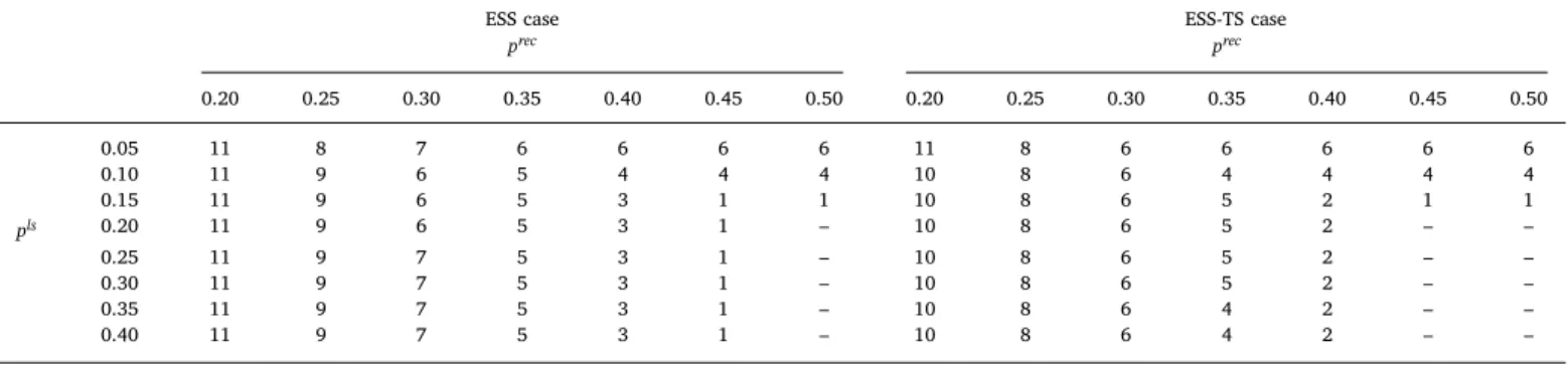
To observe the value of TS on ESS decisions, we compare the op-timal results obtained with the ESS and ESS-TS cases.Table 3presents the number of storage units, and they generally increase for both cases as we tighten pls and preclimits. We also observe that the number of storage units are highly dependent on prec values. Although varying onlyplsfor any precvalue does not change the number of ESSes in many instances, varying only prec for any pls ⩾0.2changes the number of ESSes from 11 to 0. Therefore, depending on system operators’ re-newable energy targets, ESSes can play an important role.
Our results also demonstrate that increasing the efficiency of the system with TS operations generally leads to fewer storage units needed for the same limits. We also note that ESS locations are similar in both cases, and that ESSes are generally located close to renewable genera-tion units or large convengenera-tional power plants (Fig. 1) to addflexibility to the grid to use the stored energy as required. More details about ESS locations can be found in AppendixFigs. 12–15.
Table 4presents the improvements in the total energy capacity and power rating of ESSes when TS operations are used in the power system. The value of TS is significant for instances whenpls⩾0.1and
⩽p ⩽
0.35 rec 0.4; up to 50.69% improvement on the total energy ca-pacity and 57.52% improvement on the total power rating are obtained. As discussed above, improvements decrease when pls or prec is low because investments are required in the ESS-TS case. Moreover, infive instances, when precis equal to 0.45, the storage units built in the ESS case are not needed in the ESS-TS case. Thus, 100% improvement is
obtained in these instances. Details on the energy capacity and power rating of ESSes can be found in AppendixFigs. 12–15.
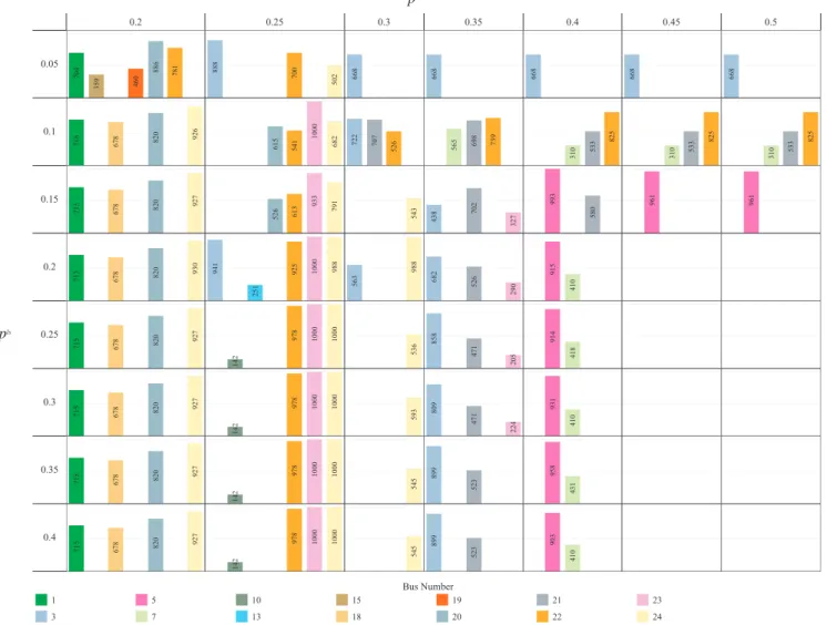
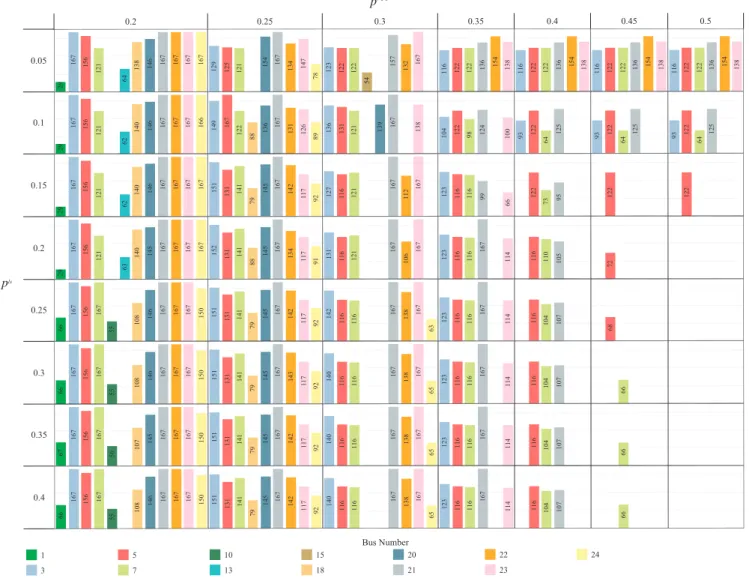
We now detail the locations and sizes of storage units for the highlighted row and columns inTable 4. In the following tables and figures, the row and the column are represented by (p pls, rec) = (0.2, :) and p( ls,prec)= (:, 0.4), respectively.Figs. 5 and 6demonstrate the total energy capacity and power rating of storage units for the ESS and ESS-TS cases with (pls,prec) = (0.2, :) and p( ls,prec)= (:, 0.4), respectively. When we relax RES generation requirements (or increase prec) for the instances withpls=0.2(Fig. 5), the total energy capacity and power rating of ESSes gradually decrease in both cases. On the other hand, relaxingpls up to 0.15, for the instances withprec=0.4 (Fig. 6), sig-nificantly reduces the energy capacity and power rating in both cases. Thus, while we conclude that energy storage is a very effective com-ponent of the system for meeting the various prec limits, the role of storage is limited to only very smallplsvalues, and the effect of TS on this role of the storage becomes more prominent as the constraints on REC and LS are relaxed.
For the results obtained with (pls,prec)= (0.2, :) and
p p
( ls, rec)= (:, 0.4),Figs. 7–10detail the results of ESS by presenting the changes in their locations and sizes when TS is incorporated into the power system. In thefigures, we only focus on the differences, and do not include storage units built at the same bus with the maximum al-lowable energy capacity or power rating in the ESS and ESS-TS cases. One canfind the storage units with the maximum sizes in both cases in AppendixTables 5 and 6. So far, we have presented that TS can de-crease the total number of storage units (Table 3) and/or the total en-ergy capacity and power rating (Table 4). These conclusions can also be observed in Figs. 7–10. For example, in the solution obtained with (pls,prec) = (0.15, 0.4), in both the ESS and ESS-TS cases, the size of the storage units located at buses 5 and 21 are almost the same. In the ESS-TS case, by not needing to build the storage at bus 7 that is located in the ESS case, the number of storage units in the system decreases by one. Even when the number and locations of storage units are the same, TS can decrease the total storage size, as in (pls,prec) = (0.2, 0.35).
Transmission switching can also affect the locations of storage units Table 3
Number of storage units.
ESS case ESS-TS case
prec prec 0.20 0.25 0.30 0.35 0.40 0.45 0.50 0.20 0.25 0.30 0.35 0.40 0.45 0.50 0.05 11 8 7 6 6 6 6 11 8 6 6 6 6 6 0.10 11 9 6 5 4 4 4 10 8 6 4 4 4 4 0.15 11 9 6 5 3 1 1 10 8 6 5 2 1 1 pls 0.20 11 9 6 5 3 1 – 10 8 6 5 2 – – 0.25 11 9 7 5 3 1 – 10 8 6 5 2 – – 0.30 11 9 7 5 3 1 – 10 8 6 5 2 – – 0.35 11 9 7 5 3 1 – 10 8 6 4 2 – – 0.40 11 9 7 5 3 1 – 10 8 6 4 2 – – Table 4
in the system. For instance, as in the solution obtained with (pls,prec) = (0.1, 0.4), in the ESS-TS case, new storage is built at bus 22 instead of at bus 2 in the ESS case. Therefore, not only for short-term operational decisions, but also for medium- to long-term planning de-cisions, as discussed in[34]without considering ESS sizing, the effect of TS can be significant depending on load targets and/or RES utilization levels.
3.2.3. Effect of TS on REC and LS
Previous sections discuss the effect of TS on the total system cost and on ESS locations and sizes. We show that TS addsflexibility to the grid, increases component efficiency and generates more electricity from RESes to meet demand. Therefore, in addition to reducing the
total system cost and storage sizes, TS inherently increases the share of RESes in the total supply.
Although the benefit of TS on REC is obvious in some instances, such as (pls,prec) = (0.2, 0.5), where the total system cost decreases due to an increase in generation from RESes, the benefit of TS on LS is not obvious due to the discretization ofplsand prec. In order to handle this deficiency and examine the effect of TS on LS, we modify the proposed model from Section 2. We provide the following multi-objective mathematical programming model that minimizes pls and prec as two conflicting objectives: min pls (35)
p
rec 0 2000 4000 6000 8000 10000MWh
(a)
ESS case0.2 0.25 0.3 0.35 0.4 0.45 0.2 0.25 0.3 0.35 0.4 0.45
p
rec 0 250 500 750 1000 1250 1500MW
(b)
ESS-TS caseFig. 5. Effect of TS on ESS sizing with p p(ls, rec)= (0.2, :) (a) energy capacity and (b) power rating.
p
ls 0 2000 4000 6000MWh
(a)
ESS case 0.1 0.2 0.3 0.4 0.1 0.2 0.3 0.4p
ls 0 250 500 750MW
(b)
ESS-TS caseFig. 6. Effect of TS on ESS sizing with p p(ls, rec)= (:, 0.4) (a) energy capacity and (b) power rating.
(pls,prec)=(0.2, 0.2) ESS ESS-TS 0 1000 2000 3000 4000 MWh (pls,prec)=(0.2, 0.25) ESS ESS-TS 0 2000 4000 6000 MWh 1 3 5 7 13 18 20 21 22 23 24 (pls,prec)=(0.2, 0.3) ESS ESS-TS 0 500 1000 1500 2000 MWh (pls,prec)=(0.2, 0.35) ESS ESS-TS 0 1000 2000 3000 MWh (pls,prec)=(0.2, 0.4) ESS ESS-TS 0 1000 2000 3000 MWh (pls,prec)=(0.2, 0.45) ESS ESS-TS 0 200 400 600 800 MWh
min prec (36)
∑ ∑
⩽∑ ∑
∀ ∈ ∈ ∈ ∈ ∈ s t. DS p D s S i B t T its ls i B t T its (20′)∑ ∑ ∑
⩾ −∑ ∑ ∑
∀ ∈ ∈ ∈ ∈ ∈ ∈ ∈ G (1 p ) G s S i B g C t T igts rec i B g C t T igts R R (21′) + + ⩽zline zstorage zom budget (37)
(2)–(5), (8)–(28) (pls,prec)=(0.2, 0.2) ESS ESS-TS 0 500 1000 MW (pls,prec)=(0.2, 0.25) ESS ESS-TS 0 500 1000 MW 1 3 5 7 13 18 20 21 22 23 24 (pls,prec)=(0.2, 0.3) ESS ESS-TS 0 200 400 600 MW (pls,prec)=(0.2, 0.35) ESS ESS-TS 0 200 400 600 800 MW (pls,prec)=(0.2, 0.4) ESS ESS-TS 0 100 200 300 400 MW (pls,prec)=(0.2, 0.45) ESS ESS-TS 0 20 40 60 80 MW
Fig. 8. Effect of TS on ESS siting and power rating for (p pls, rec) = (0.2, :).
(pls,prec)=(0.05, 0.4) ESS ESS-TS 0 500 1000 MWh (pls,prec)=(0.1, 0.4) ESS ESS-TS 0 1000 2000 3000 MWh 3 5 7 21 22 (pls,prec)=(0.15, 0.4) ESS ESS-TS 0 1000 2000 3000 MWh (pls,prec)=(0.2, 0.4) ESS ESS-TS 0 1000 2000 3000 MWh (pls,prec)=(0.25, 0.4) ESS ESS-TS 0 1000 2000 3000 MWh (pls,prec)=(0.3, 0.4) ESS ESS-TS 0 1000 2000 3000 MWh (pls,prec)=(0.35, 0.4) ESS ESS-TS 0 1000 2000 3000 MWh (pls,prec)=(0.4, 0.4) ESS ESS-TS 0 1000 2000 3000 MWh
Fig. 9. Effect of TS on ESS siting and energy capacity for (p pls, rec) = (:, 0.4).
(pls,prec)=(0.05, 0.4) ESS ESS-TS 0 200 400 600 800 MW 3 5 7 21 22 23 (pls,prec)=(0.1, 0.4) ESS ESS-TS 0 200 400 600 MW (pls,prec)=(0.15, 0.4) ESS ESS-TS 0 100 200 300 MW (pls,prec)=(0.2, 0.4) ESS ESS-TS 0 100 200 300 400 MW (pls,prec)=(0.25, 0.4) ESS ESS-TS 0 100 200 300 400 MW (pls,prec)=(0.3, 0.4) ESS ESS-TS 0 100 200 300 400 MW (pls,prec)=(0.35, 0.4) ESS ESS-TS 0 100 200 300 400 MW (pls,prec)=(0.4, 0.4) ESS ESS-TS 0 100 200 300 400 MW
In the model presented above,plsand precare the decision variables and Constraints(20′) and (21′)determine the minimumplsand precin the system, respectively. For this analysis, we also limit the total system cost with a budget represented by Constraint(37).
The ε-constraint method is a widely used approach for solving multi-objective problems [38]. In this method, one of the objective functions is selected to be optimized and the other one is added to the model as a new constraint with a bound. In this study, a variation of this method is used to obtain only non-dominated solutions. In the aug-mentedε-constraint method[38], the second objective is also added to the objective function by multiplying with a small coefficient,γ. By sequentially increasing/decreasing the bound of the second objective,ε, all Pareto-optimal solutions are found. The objective function and the new constraint added to the model to solve the problem with the
ε-constraint method is represented as follows: +
min pls γprec (38)
⩽
prec ε (39)
For discussing the effect of TS on REC and LS, we utilize the solution obtained with (pls,prec) = (0.2, 0.4) for the ESS case and limit the total system cost by $148.741 M, which is the optimal solution value of that instance.
Fig. 11demonstrates the sets of pareto optimal solutions for the ESS and ESS-TS cases. Transmission switching operations improve the effi-ciency of the power system and yield to lower preclimits for the same
pls. Moreover, TS operations decrease the minimumplslimit from 0.18
to 0.16. We also emphasize that the highest RES penetration level, (i.e. the lowest prec) in the ESS case (37.71%) is worse than the lowest RES penetration level, (i.e the highest prec) in the ESS-TS case (37.75%). Hence, TS helps system operators increase the share of RES in the total supply and improve quality of life without allocating more resources. We note that these results are clearly dependent on a predetermined budget, and therefore, the value of TS could be more significant with budget limits other than the one presented here.
4. Conclusion
This paper provides a mathematical model that co-optimizes transmission switching operations, ESS siting and sizing decisions and considering limits on maximum allowable load shedding and renewable energy curtailment amounts in the power system. Utilizing an extensive computational study on the IEEE 24-bus power system, we precisely characterize the effect of transmission switching on total system cost, ESS locations and sizes, load shedding and renewable energy curtail-ment control mechanisms. Our results provide insights about the role of storage at different limits for load shedding and renewable energy curtailment control mechanisms; the modeling framework discussed in this study can also be extended to optimizing storage portfolios for power systems. Our results show that total system cost and total ESS size can be decreased up to 17% and 50%, respectively, and the full potential of ESS in the power system can be revealed for a vertically integrated utility when switching operations are utilized. The results also demonstrate that switching lines helps system operators use their budgets to apply better demand-side management and/or renewable energy curtailment policies due to increased utilization of system components.
In this paper, we present a static planning model to constitute a balance between computational complexity and solution quality. However, this model can easily be adapted to the dynamic planning problem, where (with increased solution time) the time of building new transmission lines and storage units can be determined. Moreover, in-corporating features such as start-up and shut-down status of conven-tional plants leads to a problem with more computaconven-tional complexity. Thus, good heuristics and/or sophisticated solution techniques could be future research directions to explore applying this problem to larger and real-world power systems.
Appendix A Tables 5 and 6 0.16 0.18 0.2 0.22 0.24 0.26 0.28 0.3 0.32 0.34 pls 0.34 0.36 0.38 0.4 0.42 p rec ESS case ESS-TS case
Fig. 11. Effect of TS on REC and LS with a $148.741 M budget for the total system cost.
Table 5
ESS locations with maximum energy capacity common to the ESS and ESS-TS cases.
prec 0.20 0.25 0.30 0.35 0.40 0.45 0.50 0.05 3, 5, 7, 21, 23, 24 5, 7, 20, 21, 23 5, 7, 21, 22, 23 5, 7, 21, 22, 23 5, 7, 21, 22, 23 5, 7, 21, 22, 23 5, 7, 21, 22, 23 0.10 3, 5, 7, 21, 22, 23 3, 5, 7, 21 5, 7, 23 5 5 5 5 0.15 3, 5, 7, 21, 22, 23 3, 5, 7, 21 3, 5, 7, 21, 23 5, 7 – – – pls 0.20 3, 5, 7, 21, 22, 23 5, 7, 21 5, 7, 21, 23 5, 7 – – – 0.25 3, 5, 7, 21, 22, 23 3, 5, 7, 21 3, 5, 7, 21, 23 5, 7 – – – 0.30 3, 5, 7, 21, 22, 23 3, 5, 7, 21 3, 5, 7, 21, 23 5, 7 – – – 0.35 3, 5, 7, 21, 22, 23 3, 5, 7, 21 3, 5, 7, 21, 23 5, 7 – – – 0.40 3, 5, 7, 21, 22, 23 3, 5, 7, 21 3, 5, 7, 21, 23 5, 7 – – –
Figs. 12–15 Table 6
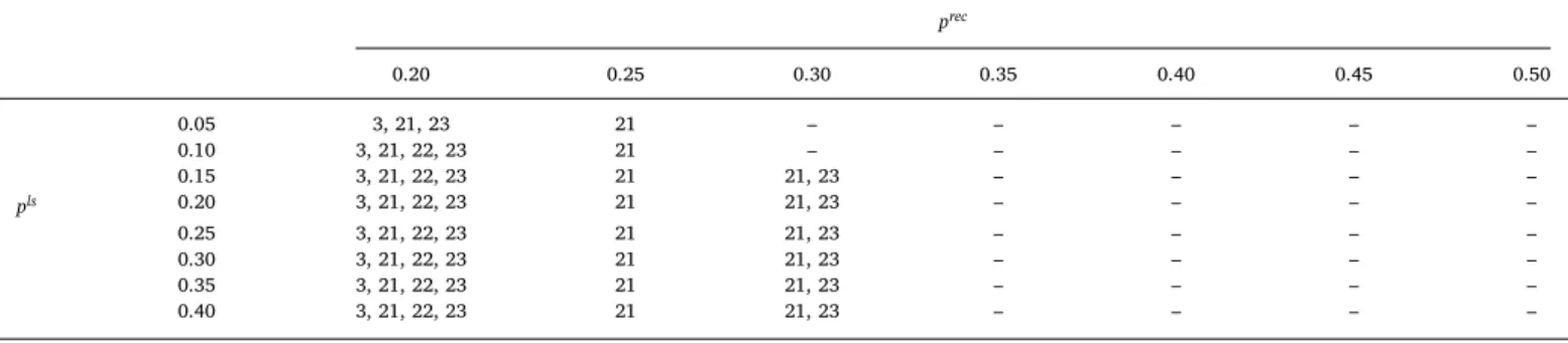
ESS locations with maximum power rating common to the ESS and ESS-TS cases.
prec 0.20 0.25 0.30 0.35 0.40 0.45 0.50 0.05 3, 21, 23 21 – – – – – 0.10 3, 21, 22, 23 21 – – – – – 0.15 3, 21, 22, 23 21 21, 23 – – – – pls 0.20 3, 21, 22, 23 21 21, 23 – – – – 0.25 3, 21, 22, 23 21 21, 23 – – – – 0.30 3, 21, 22, 23 21 21, 23 – – – – 0.35 3, 21, 22, 23 21 21, 23 – – – – 0.40 3, 21, 22, 23 21 21, 23 – – – –
p
recp
lsp
recp
lsp
recp
lsReferences
[1] Zhou Ying, Wang Lizhi, McCalley James D. Designing effective and efficient in-centive policies for renewable energy in generation expansion planning. Appl Energy 2011;88(6):2201–9.
[2] International Energy Agency. World Energy Outlook-2017. OECD/IEA; 2017. p. 257.
[3] Moura Pedro S, De Almeida Anibal T. The role of demand-side management in the grid integration of wind power. Appl Energy 2010;87(8):2581–8.
[4] Kocaman Ayse Selin, Modi Vijay. Value of pumped hydro storage in a hybrid energy generation and allocation system. Appl Energy 2017;205:1202–15.
[5] Yuan Shengxi, Kocaman Ayse Selin, Modi Vijay. Benefits of forecasting and energy storage in isolated grids with large wind penetration–the case of Sao Vicente. Renew Energy 2017;105:167–74.
[6] Vargas Luis S, Bustos-Turu Gonzalo, Larraín Felipe. Wind power curtailment and energy storage in transmission congestion management considering power plants ramp rates. IEEE Trans Power Syst 2015;30(5):2498–506.
[7] Jennifer Rogers, Sari Fink, Kevin Porter. Examples of wind energy curtailment practices; 2010 <https://www.nrel.gov/docs/fy10osti/48737.pdf> .
[8] Fisher Emily B, O’Neill Richard P, Ferris Michael C. Optimal transmission switching.
IEEE Trans Power Syst 2008;23(3):1346–55.
[9] Bhattacharya Mita, Paramati Sudharshan Reddy, Ozturk Ilhan, Bhattacharya Sankar. The effect of renewable energy consumption on economic growth: evidence from top 38 countries. Appl Energy 2016;162:733–41.
[10] Finn Paddy, Fitzpatrick Colin. Demand side management of industrial electricity consumption: promoting the use of renewable energy through real-time pricing. Appl Energy 2014;113:11–21.
[11] Pandžić Hrvoje, Wang Yishen, Qiu Ting, Dvorkin Yury, Kirschen Daniel S. Near-optimal method for siting and sizing of distributed storage in a transmission net-work. IEEE Trans Power Syst 2015;30(5):2288–300.
[12] Li Nan, Hedman Kory W. Economic assessment of energy storage in systems with
high levels of renewable resources. IEEE Trans Sustain Energy 2015;6(3):1103–11. [13] Hedayati Mojgan, Zhang Junshan, Hedman Kory W. Joint transmission expansion planning and energy storage placement in smart grid towards efficient integration of renewable energy. In: T&D Conference and Exposition, 2014 IEEE PES. IEEE; 2014. p. 1–5.
[14] Jabr Rabih A, Džafić Izudin, Pal Bikash C. Robust optimization of storage invest-ment on transmission networks. IEEE Trans Power Syst 2015;30(1):531–9. [15] Conejo Antonio J, Cheng Yaohua, Zhang Ning, Kang Chongqing. Long-term
co-ordination of transmission and storage to integrate wind power. CSEE J Power Energy Syst 2017;3(1):36–43.
[16] Bucciarelli Martina, Paoletti Simone, Vicino Antonio. Optimal sizing of energy storage systems under uncertain demand and generation. Appl Energy 2018;225:611–21.
[17] Wogrin Sonja, Gayme Dennice F. Optimizing storage siting, sizing, and technology portfolios in transmission-constrained networks. IEEE Trans Power Syst 2015;30(6):3304–13.
[18] Fernández-Blanco Ricardo, Dvorkin Yury, Xu Bolun, Wang Yishen, Kirschen Daniel S. Optimal energy storage siting and sizing: a WECC case study. IEEE Trans Sustain Energy 2017;8(2):733–43.
[19] Go Roderick S, Munoz Francisco D, Watson Jean-Paul. Assessing the economic value of co-optimized grid-scale energy storage investments in supporting high renewable portfolio standards. Appl Energy 2016;183:902–13.
[20] Xiong Peng, Singh Chanan. Optimal planning of storage in power systems in-tegrated with wind power generation. IEEE Trans Sustain Energy
2016;7(1):232–40.
[21] Qiu Ting, Xu Bolun, Wang Yishen, Dvorkin Yury, Kirschen Daniel S. Stochastic multistage coplanning of transmission expansion and energy storage. IEEE Trans Power Syst 2017;32(1):643–51.
[22] Hedman KW, O’Neill RP, Fisher EB, Oren SS. Optimal transmission switching with contingency analysis. IEEE Trans Power Syst 2009;24(3):1577–86.
[23] W. Hedman K, Ferris MC, O’Neill RP, Fisher EB, Oren SS. Co-optimization of gen-eration unit commitment and transmission switching with N-1 reliability. IEEE
p
recp
lsTrans Power Syst 2010;25(2):1052–63.
[24] Jabarnejad M, Wang J, Valenzuela J. A decomposition approach for solving sea-sonal transmission switching. IEEE Trans Power Syst 2015;30(3):1203–11. [25] Khodaei A, Shahidehpour M, Kamalinia S. Transmission switching in expansion
planning. IEEE Trans Power Syst 2010;25(3):1722–33.
[26] Hedman KW, Shmuel S. Oren, Richard P. O’Neill. A review of transmission switching and network topology optimization. In: Power and energy society general meeting, 2011 IEEE. IEEE; 2011. p. 1–7.
[27] Evgeniy A. Goldis, Xiaoguang Li, Michael C. Caramanis, Bhavana Keshavamurthy, Mahendra Patel, Aleksandr M. Rudkevich, et al. Applicability of topology control algorithms (TCA) to a real-size power system. In: 2013 51st Annual Allerton con-ference on communication, control, and computing (Allerton). IEEE; 2013. p. 1349–52.
[28] Pablo A. Ruiz, Michael Caramanis, Evgeniy Goldis, Bhavana Keshavamurthy, Xiaoguang Li, Russ Philbrick, et al. Topology control algorithms (TCA) simulations in PJM with AC modeling. In: Technical conference on increasing real-time and day-ahead market efficiency through improved software, Washington. FERC; 2014. [29] Villumsen Jonas Christoffer, Bronmo Geir, Philpott Andy B. Line capacity expansion
and transmission switching in power systems with large-scale wind power. IEEE Trans Power Syst 2013;28(2):731–9.
[30] Qiu Feng, Wang Jianhui. Chance-constrained transmission switching with guaran-teed wind power utilization. IEEE Trans Power Syst 2015;30(3):1270–8. [31] Nikoobakht Ahmad, Aghaei Jamshid, Mardaneh Mohammad. Securing highly
pe-netrated wind energy systems using linearized transmission switching mechanism.
Appl Energy 2017;190:1207–20.
[32] Nikoobakht Ahmad, Aghaei Jamshid, Mardaneh Mohammad. Managing the risk of uncertain wind power generation inflexible power systems using information gap decision theory. Energy 2016;114:846–61.
[33] Aghaei Jamshid, Nikoobakht Ahmad, Mardaneh Mohammad, Shafie-khah Miadreza, Catal ao Jo ao PS. Transmission switching, demand response and energy storage systems in an innovative integrated scheme for managing the uncertainty of wind power generation. Int J Electr Power Energy Syst 2018;98:72–84. [34] Dehghan Shahab, Amjady Nima. Robust transmission and energy storage expansion
planning in wind farm-integrated power systems considering transmission switching. IEEE Trans Sustain Energy 2016;7(2):765–74.
[35] Krishnan Venkat, Ho Jonathan, Hobbs Benjamin F, Liu Andrew L, McCalley James D, Shahidehpour Mohammad, et al. Co-optimization of electricity transmission and generation resources for planning and policy analysis: review of concepts and modeling approaches. Energy Syst 2016;7(2):297–332.
[36] Cliff Grigg, et al. The IEEE reliability test system-1996. IEEE Trans Power Syst 1999;14(3):1010–20.
[37] Altıntaş Onur, Okten Busra, Karsu Özlem, Kocaman Ayse Selin. Bi-objective opti-mization of a grid-connected decentralized energy system. Int J Energy Res 2018;42(2):447–65.
[38] Mavrotas George. Effective implementation of theε-constraint method in multi-objective mathematical programming problems. Appl Math Comput