* Corresponding Author
Numerical Approximation of the Combined KdV-mKdV Equation via the Quintic B-Spline Differential Quadrature Method
N. Murat YAĞMURLU1,*, Yusuf UÇAR2, Ali BAŞHAN3
1İnönü University, Faculty of Science and Art, Department of Mathematics, Malatya, Turkey [email protected], ORCID: 0000-0003-1593-0254
2İnönü University, Faculty of Science and Art, Department of Mathematics, Malatya, Turkey [email protected], ORCID: 0000-0003-1469-5002
3Zonguldak Bülent Ecevit University, Faculty of Science and Art, Department of Mathematics, Zonguldak, Turkey
[email protected], ORCID: 0000-0001-8500-493X
Abstract
In this paper, quintic B-spline differential quadrature method (QBDQM) has been used to obtain the numerical approximation of the combined Korteweg-de Vries and modified Korteweg-de Vries equation (combined KdV-mKdV). The efficiency and effectiveness of the proposed method has been tested by computing the maximum error norm 𝐿" and discrete root mean square error 𝐿#. The newly found numerical approximations have been compared to available numerical approximations and this comparison has shown that the proposed method is an efficient one for solving the combined KdV-mKdV equation. We have also carried out a stability analysis.
Keywords: Partial differential equations, Differential quadrature method,
Combined KdV-mKdV equation, Quintic B-Splines, Strong stability-preserving Runge-Kutta method.
Adıyaman University Journal of Science
https://dergipark.org.tr/en/pub/adyujsci DOI: 10.37094/adyujsci.526264
ADYUJSCI 9 (2) (2019)
Kombine KdV-mKdV Denkleminin Kuintik B-Splayn Diferansiyel Kuadratür Yöntemiyle Sayısal Yaklaşımlar
Öz
Bu makalede, kombine Korteweg-de Vries ve modifiye edilmiş Korteweg-de Vries denkleminin (kombine KdV-mKdV) sayısal yaklaşımını elde etmek için kuintik B-spline diferansiyel kuadratür yöntemi (QBDQM) uygulanmıştır. Yöntemin etkinliği ve doğruluğu, maksimum hata normu 𝐿" ve ayrık kök ortalama kare hatası 𝐿# hesaplanarak ölçülmüştür. Yeni elde edilen sayısal sonuçlar, yayınlanan sayısal sonuçlarla karşılaştırıldı ve karşılaştırma, yöntemin, kombine KdV-mKdV denklemini çözmek için etkili bir sayısal şema olduğunu göstermiştir. Aynı zamanda bir kararlılık analizi de yapılmıştır.
Anahtar Kelimeler: Kısmi diferansiyel denklemler, Diferansiyel kuadratür metod,
Kombine KdV-mKdV denklemi, Kuintik B-Splaynlar, Güçlü kararlılık-koruyucu Runge-Kutta metod
1. Introduction
In this study, we are going to investigate one of the widely used natural phenomena which is also a prototype for wave propagation in a 1-dimensional nonlinear lattice [1, 2]. Because of its importance, many researchers have dealt with the combined KdV-mKdV equation given as
𝑈%+ 6𝛼𝑈𝑈) + 6𝛽𝑈#𝑈
) + 𝑈))) = 0, (1) in which 𝛼 and 𝛽 denote constant parameters, 𝑡 and 𝑥 stand for time and space derivatives, respectively.
Combined KdV-mKdV equation is solved with various methods by several researchers. It has both analytical and numerical solutions. Among others, Ablowitz and Taha found differential-difference equations having as limiting forms the KdV and mKdV equations [3]. Fan [4] proposed a novel unified algebraic procedure for constructing a series of explicit analytic solutions about general nonlinear equations. Peng [5] developed the modified mapping method for finding novel analytic solutions of the
combined KdV-mKdV equation. Bekir [6] established analytic solutions of combined KdV-mKdV equation with extended tanh method. Lu and Shi [7] established analytic solutions of combined KdV-mKdV equation by using four novel types of Jacobi elliptic funtions and extending the Jacobi elliptic functions. Taha [3] implemented inverse scattering transform numerical procedure for nonlinear evolution equations.
As an effective method for obtaining approximate solutions via small number of nodal points, Bellman et al. [8] first presented DQM in 1972 where partial derivative of a function in terms of a coordinate direction is defined as a linear weighted combination of the functional values over the nodes on the given direction [9]. The method has been popular recently due to its easy application. The basic concept of the method is to find the weighting coefficients for functional values at nodes by using the base functions whose derivatives are known on the same nodes over the solution domain. Several scholars presented various types of DQM by using several trial functions. For example, Bellman et al. [8, 10] utilized Legendre polynomials with spline base functions for finding weighting coefficients. Quan and Chang [11, 12] presented an explicit formula to find out the weighting coefficients by means of Lagrange interpolation polynomials. Shu and Richards [13] introduced an explicit formula including Lagrange interpolation polynomials. Besides those, Shu and Xue [14] used Lagrange interpolated trigonometric polynomials for finding out weighting coefficients explicitly. Zhong [15], Guo and Zhong [16] and Zhong and Lan [17] presented an effective DQM as spline based DQM and tested it on several problems. Cheng et al. [18] proposed Hermite polynomials to determine the weighting coefficients. Shu and Wu [19] have presented a few implicit formulations of weighting coefficients based on radial base functions. The weighting coefficients are at the same time found by Striz et al. [20] with harmonic functions. Sinc functions are utilized as base functions in finding the weighting coefficients by Korkmaz and Dağ [21] and Bonzani [22]. B-spline base functions are also used to find weighting coefficients by Başhan [23], and Korkmaz and Dağ [24-26].
In this manuscript, QBDQM will be used for finding numerical solutions of the combined KdV-mKdV equation. DQM based on cubic B-spline has been utilized to solve the 312 order differential equations such as KdV one which needs to be transformed for solution [27]. However, QBDQM doesn’t need transformation to solve the 312 order
differential equations such as KdV, combined KdV-mKdV and to carry out the stability analysis of the present method there is no need for a reduction like splitting for the solution procedure. Thus, to be able to carry out stability analysis of the 312 order non-linear combined KdV-mKdV equation, quintic B-spline basis functions have been preferred. The DQM has many pros over the classical methods, chiefly, it doesn’t require perturbation and linearization to get more accurate solutions for a given nonlinear equation.
2. Application of the Method
DQM is described as an approximation for derivatives of a predfined function by means of the linear combination of the functional values at nodal points on the solution domain of the problem. When we assume 𝑎 = 𝑥4 < 𝑥# < ⋯ < 𝑥7= 𝑏 on the closed interval 𝑎, 𝑏 . If 𝑈 𝑥 is smooth enough on its domain, then the derivatives of itself in terms of 𝑥 at node 𝑥9 is written as linear combination of its functional values, that is,
𝑈)1 𝑥9 = 2
:;
2): |)= = 7>?4 𝑤9>
1 𝑈 𝑥
> , 𝑖 = 1(1)𝑁, 𝑟 = 1(1)𝑁 − 1, (2)
here 𝑟 is derivative order, 𝑤9>1 are the weighting coefficients denoting 𝑟%I order derivative approximation, 𝑁 is the number of nodes. The 𝑗 is a symbol stating that 𝑤9>1 is the weighting coefficient for the value 𝑈 𝑥> .
In the present work, we are going to need the 1K% and 312 order derivatives for the function 𝑈(𝑥). Thus, we are going to find the values of the Eq. (2) for the 𝑟 = 1,3.
When Eq. (2) is scrutinized, then one can see that the basic procedure of approximating the derivatives of a predefined function by means of DQM is about finding the unknown coefficients 𝑤9>1 . The basic idea lying under DQM is about finding the unknown weighting coefficients 𝑤9>1 through base functions covering the solution domain. In this process, various base functions can be applied. For this manuscript, we are going to calculate weighting coefficients by means of quintic B-spline base functions. If we assume 𝑄N(𝑥) are the quintic B-spline base functions with nodes 𝑥9 in which the uniform 𝑁 nodes are used as 𝑎 = 𝑥4 < 𝑥# < ⋯ < 𝑥7= 𝑏 on the space axis. Then the
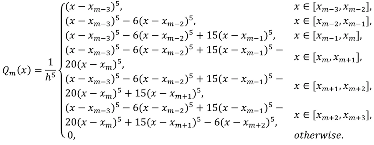
set of B-splines 𝑄9 for 𝑖 = −1(1)𝑁 + 2 constitutes a base for the functions on [𝑎, 𝑏]. The quintic B-splines 𝑄N(𝑥) are described by the following relationships:
𝑄N 𝑥 = 1 ℎR (𝑥 − 𝑥NST)R, 𝑥 ∈ [𝑥 NST, 𝑥NS#], (𝑥 − 𝑥NST)R− 6(𝑥 − 𝑥 NS#)R, 𝑥 ∈ [𝑥NS#, 𝑥NS4], (𝑥 − 𝑥NST)R− 6(𝑥 − 𝑥 NS#)R+ 15(𝑥 − 𝑥NS4)R, 𝑥 ∈ [𝑥NS4, 𝑥N], (𝑥 − 𝑥NST)R− 6(𝑥 − 𝑥 NS#)R+ 15(𝑥 − 𝑥NS4)R− 20(𝑥 − 𝑥N)R, 𝑥 ∈ [𝑥N, 𝑥NW4], (𝑥 − 𝑥NST)R− 6(𝑥 − 𝑥 NS#)R+ 15(𝑥 − 𝑥NS4)R− 20(𝑥 − 𝑥N)R+ 15(𝑥 − 𝑥 NW4)R, 𝑥 ∈ [𝑥NW4, 𝑥NW#], (𝑥 − 𝑥NST)R− 6(𝑥 − 𝑥 NS#)R+ 15(𝑥 − 𝑥NS4)R− 20(𝑥 − 𝑥N)R+ 15(𝑥 − 𝑥 NW4)R− 6(𝑥 − 𝑥NW#)R, 𝑥 ∈ [𝑥NW#, 𝑥NWT], 0, 𝑜𝑡ℎ𝑒𝑟𝑤𝑖𝑠𝑒.
where ℎ = 𝑥N− 𝑥NS4 for all 𝑚 [28]. The values of quintic B-splines and its derivatives at the grid points are given in Table 1.
Table 1. The values of quintic and its derivative functions at the grid points
2.1. Determination of the First Order Derivative Weighting Coefficients
In Eq. (2) if we take 𝑟 = 1 and use quintic B-splines as trial functions we obtain the following equations
𝑄] ^
𝑥9 = ]W#
>?]S# 𝑤9,>4 𝑄] 𝑥> , 𝑘 = −1(1)𝑁 + 2, 𝑖 = 1(1)𝑁. (3) For instance, for the 1K% nodal point 𝑥
4 (3), we obtain the following equation 𝑄] ^
𝑥4 = ]W#
>?]S# 𝑤4,>4 𝑄] 𝑥> , 𝑘 = −1,0, … , 𝑁 + 2. (4) When we place the value of quintic basis functions in Eq. (4) and use four additional equations which are obtained from derivative of Eq. (4) at four different B-spline 𝑄] 𝑘 = −1,0, 𝑁 + 1, 𝑁 + 2 and finally eliminate four unknown terms from equation system, we obtain the following system of equations:
𝑥 𝑥NST 𝑥NS# 𝑥NS4 𝑥N 𝑥NW4 𝑥NW# 𝑥NWT 𝑄N 0 1 26 66 26 1 0 𝑄N ^ 0 R I Rb I 0 − Rb I − R I 0 𝑄N ^^ 0 I#bc Idbc −4#bIc dbIc I#bc 0 𝑄N ^^^ 0 Iebf −4#bIf 0 4#bIf −Iebf 0 𝑄Nd 0 4#bIg dhbIg i#bIg −dhbIg 4#bIg 0
(5)
Similarly, by using the value of quintic basis functions at the 𝑥9, 2 ≤ 𝑖 ≤ 𝑁 − 1 grid points, respectively, the following equation system is obtained:
(6)
For the last grid point 𝑥7 the following equation system is obtained:
So, weighting coefficients 𝑤9,>4 which are related to the 𝑥9, 𝑖 = 1,2, . . . , 𝑁 are found quite easily by solving equation systems (5), (6) and (7) with Thomas algorithm.
2.2. Determination of the Third Order Derivative Weighting Coefficients
We will obtain the weighting coefficients of the 312 order derivatives similarly. In Eq. (2) if we take 𝑟 = 3, we obtain
𝑄] ^^^ 𝑥
9 = ]W#>?]S# 𝑤9,>T 𝑄] 𝑥> , 𝑘 = −1,0, … , 𝑁 + 2, 𝑖 = 1,2, . . . , 𝑁. (8) For the 1K% node 𝑥
4 (8), we obtain the following equation 𝑄] ^^^ 𝑥
4 = ]W#>?]S# 𝑤4,>T 𝑄] 𝑥> , 𝑘 = −1,0, … , 𝑁 + 2. (9) If we place the value of quintic base functions in Eq. (9) and use÷ four additional equations obtained from the derivative of Eq. (9) at points 𝑥] for 𝑘 = −1,0, 𝑁 + 1, 𝑁 + 2 and then eliminate those unknown terms from the system; the following is obtained:
(10)
Similarly, by using the value of quintic basis functions at the 𝑥9, 2 ≤ 𝑖 ≤ 𝑁 − 1 grid points, respectively, the following equation system is obtained:
(11)
For the last grid point 𝑥7 the following equation system is obtained:
(12)
So, weighting coefficients 𝑤9,>T which are related to the 𝑥9, 𝑖 = 1(1)𝑁 are found by solving equation systems 10 , (11) and (12) with Thomas algorithm.
3. Discretization Process
The combined KdV-mKdV equation of the form 𝑈%+ 6𝛼𝑈𝑈) + 6𝛽𝑈#𝑈
) + 𝑈))) = 0 (13)
having the following boundary conditions taken from 𝑈 𝑎, 𝑡 = 𝑔4 𝑡 , 𝑈 𝑏, 𝑡 = 𝑔# 𝑡
and the following initial condition
𝑈 𝑥, 0 = 𝑓4 𝑥 , 𝑎 ≤ 𝑥 ≤ 𝑏,
is rewritten as follows
𝑈% = −6𝛼𝑈𝑈) − 6𝛽𝑈#𝑈) − 𝑈))). (14) DQM approximations of the 1K% and the 312 orders are used in Eq. (14)
2; )= 2% = −6𝛼𝑈 𝑥9, 𝑡 − 6𝛽𝑈 # 𝑥 9, 𝑡 7S4>?# 𝑤9,>4 𝑈 𝑥>, 𝑡 − 7S4 >?# 𝑤9,>T 𝑈 𝑥>, 𝑡 + 𝐵9, 𝑖 = 2,3, . . . , 𝑁 − 1, (15) where 𝐵9 = −6𝛼𝑈 𝑥9, 𝑡 − 6𝛽𝑈# 𝑥 9, 𝑡 𝑤9,44 𝑔4 𝑡 + 𝑤9,74 𝑔# 𝑡 − 𝑤9,4T 𝑔4 𝑡 + 𝑤9,7T 𝑔# 𝑡
and ODE in Eq. (15) is found. Under these conditions, the integral of ODE given by Eq. (15) is taken in time using an appropriate method. Here, strong stability-preserving low storage Runge-Kutta 4(3)5 3𝑆∗ method has been preferred [29] thanks to its pros such as efficiency, stability and less memory usage characteristics.
4. Stability
Stability analysis of the numerical procedure used for a nonlinear differential equation needs the finding of eigenvalues of its coefficient matrices. With the numerical discretization of partial differential equation combined KdV-mKdV, it turns into an ODE.
The stability of a problem which is time dependent is given as t;
t% = 𝑙 𝑈 , (16) having appropriate initial and boundary conditions, in which 𝑙 stands for a spatial differential operator. When DQM is applied, Eq.(16) becomes a set of ODEs in time as
2{w}2% = 𝐴 𝑢 + 𝑏 , (17) where {𝑢} is a unknown vector of the values of the given function at the nodes except the both boundary nodes, {𝑏} is the vector including the non-homogenous part and the boundary conditions and 𝐴 is the coefficient matrix. The numerical scheme’s stability for numerical integration of Eq. (17) is dependent upon the stability of the ODE in Eq. (17). If Eq. (17) is not stable, then the numerical procedures may produce unconvergent solutions. The stability condition of Eq. (17) is closely related with the eigenvalues of the matrix 𝐴, for the exact solution is directly desribed with the eigenvalues of this matrix. If all 𝑅𝑒 𝜆9 ≤ 0 for every 𝑖, it is enough to show the stability of the analytic solution of {𝑢} when 𝑡 → ∞ where 𝑅𝑒 𝜆9 stands for the real part of the eigenvalues 𝜆9 of the matrix 𝐴. The matrix 𝐴 at Eq. (17) is found as 𝐴9> = −6𝛼𝛿9 − 6𝛽𝛿9# 𝑤
9,>4 − 𝑤9,>T where 𝛿9 = 𝑈(𝑥9, 𝑡) [23]. Those eigenvalues for matrix 𝐴 must be lying in the stability region as illustrated in Ref. [30].
5. Numerical Examples and Stability Analysis
In the present section, we are going to obtain the approximate solutions of the combined KdV-mKdV equation using the QBDQM. The efficiency of the proposed method is tested with those error norms 𝐿# and 𝐿" defined as, respectively:
𝐿# = 𝑈€•€‚ƒ%9„ − 𝑈 7 # ≃ ℎ 7 >?4 𝑈>€•€‚ƒ%9„− 𝑈7 > #, 𝐿"= 𝑈€•€‚ƒ%9„ − 𝑈 7 " ≃ max> 𝑈> €•€‚ƒ%9„− 𝑈 7 > , 𝑗 = 1(1)𝑁 − 1.
We are going to compute the numerical solutions of three different test problems using QBDQM.
5.1. Motion of Single Soliton
The analytic soliton solution of combined KdV-mKdV equation is given in [26] as:
𝑈 𝑥, 𝑡 = ‰
Š‹Œ•Žc •
c ‰ )S‰%S•‘ W’•“”Žc •c ‰ )S‰%S•‘
, (18) in which 𝜉b stands for the integration constant and
𝐶 = 𝛼#+ 𝛽𝜆 + 𝛼, 𝐷 = 𝛼#+ 𝛽𝜆 − 𝛼.
When 𝛼 = 1, 𝛽 = 1, 𝜆 = 1 and 𝜉b = 0 are taken at 𝑡 = 0, we get the initial condition. By the same thought, if we take 𝑥 = −30 and 𝑥 = 70, we obtain boundary conditions, respectively.
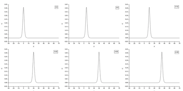
During the simulation, we have selected the several time increments and space increments over the interval −30,70 . The characteristics of the approximate solutions for Δ𝑡 = 0.01 and 𝑁 = 301 are illustrated in Fig. 1. As one can see from the Fig. 1, the amplitude and velocity of wave remain as a result of properties of solitons during the run-time.
Figure 1. Behaviour of numerical solutions at various times for Δ𝑡 = 0.01
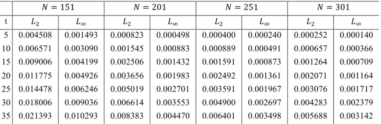
The calculated and compared values of the error norms 𝐿# and 𝐿" are given at some chosen times till 𝑡 = 35. The newly obtained results are tabulated in Table 2, Table 3 and Table 4. As one can see obviously the from Table 2 and Table 3 the present error norms 𝐿# and 𝐿" are smaller than earlier works [26] which are obtained by inverse scattering
transform (IST) and Combination IST methods. Also, it is obviously seen from Table 3 that obtained solutions by QBDQM with less number of nodes such as 𝑁 = 301 are better than those of both of the earlier works. Approximate values using different number of nodes are also shown in Table 4. It is clearly seen in Table 4 that by the increasing the number of nodes from 𝑁 = 151 to 𝑁 = 301 the 𝐿# and 𝐿" error norms decrease.
Table 2. A comparison of 𝐿# and 𝐿" error norms for 𝑁 = 200, Δ𝑡 = 0.01
Present IST [3] Com.IST [3]
t 𝐿# 𝐿" 𝐿# 𝐿" 𝐿# 𝐿"
5 0.000823 0.000498 0.00229 0.01234 0.00751 0.04293 35 0.008383 0.004470 0.00563 0.03237 0.03792 0.20920 Table 3. A comparison of 𝐿# and 𝐿" error norms for 𝑁 = 400, Δ𝑡 = 0.01
Present 𝑁 = 301 IST [3] 𝑁 = 400 Com.IST [3] 𝑁 = 400 t 𝐿# 𝐿" 𝐿# 𝐿" 𝐿# 𝐿" 5 0.000252 0.000140 0.00051 0.00313 0.00215 0.01263 35 0.005688 0.003142 0.00124 0.00701 0.01164 0.06360
Table 4. The values of 𝐿# and 𝐿" error norms for Δ𝑡 = 0.01 at various values of 𝑁
𝑁 = 151 𝑁 = 201 𝑁 = 251 𝑁 = 301 t 𝐿# 𝐿" 𝐿# 𝐿" 𝐿# 𝐿" 𝐿# 𝐿" 5 0.004508 0.001493 0.000823 0.000498 0.000400 0.000240 0.000252 0.000140 10 0.006571 0.003090 0.001545 0.000883 0.000889 0.000491 0.000657 0.000366 15 0.009006 0.004199 0.002506 0.001432 0.001591 0.000873 0.001264 0.000709 20 0.011775 0.004926 0.003656 0.001983 0.002492 0.001361 0.002071 0.001164 25 0.014478 0.006246 0.005019 0.002701 0.003591 0.001967 0.003076 0.001717 30 0.018006 0.009036 0.006614 0.003553 0.004900 0.002697 0.004283 0.002379 35 0.021393 0.010293 0.008383 0.004470 0.006401 0.003498 0.005688 0.003142
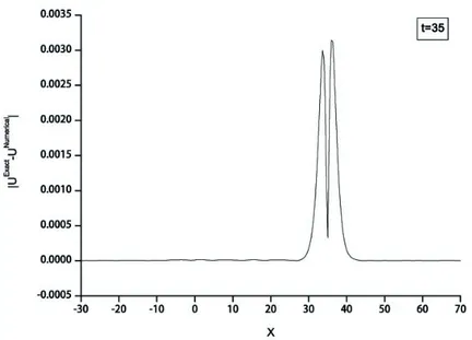
Absolute errors at time 𝑡 = 35 are given in Fig. 2. One can see from Fig. 2 that the maximum absolute error is found 0.00314 at 𝑥 = 36.
Figure 2. The graph of absolute errors at -30 ≤ 𝑥 ≤ 70, Δ𝑡 = 0.01, and N=301 at time t=35
5.2. A Bell-shaped Soliton Solution
For the present case, we are going to deal with numerical solutions of combined KdV-mKdV equation of which analytic solution is given in [7] as:
𝑈(𝑥, 𝑡) = − 𝑝 2𝑞+ 6𝑐# 𝑞 secℎ 𝑐#𝜉 , 𝑞 > 0, 𝑐# > 0, where 𝑝 = 6𝛼, 𝑞 = 6𝛽,and 𝜉 = 𝑥 + 𝑝# + 4𝑞𝑐 # /4𝑞 𝑡.
We have obtained initial condition from analytical solution at 𝑡 = 0 by using 𝑝 = 𝑞 = 1 in the following form
𝑈(𝑥, 0) = − 𝑝 2𝑞+
6𝑐#
𝑞 secℎ 𝑐#𝑥
and by the same process, if we take 𝑥 = −50 and 𝑥 = 50, we simply obtain boundary conditions.
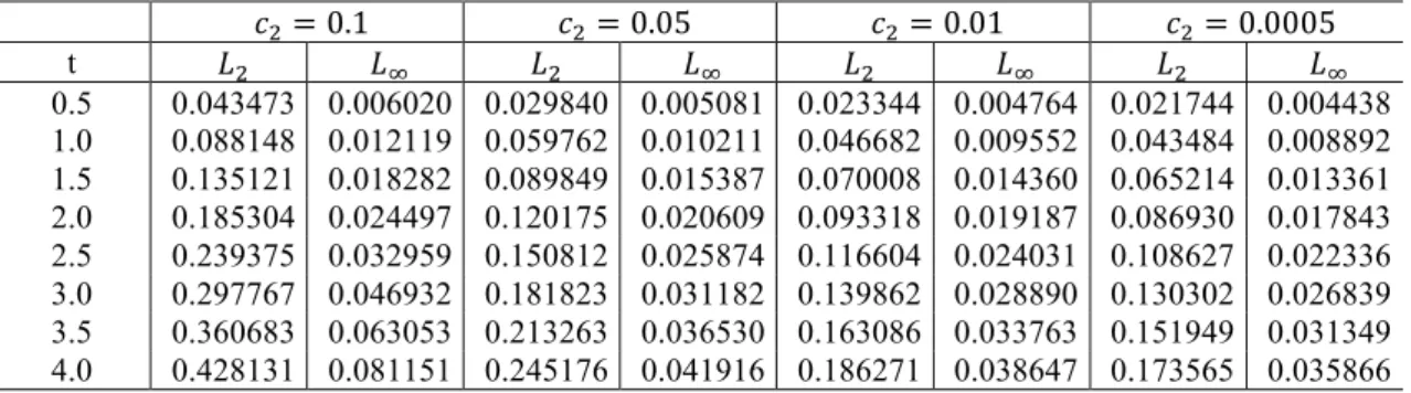
The calculated values for 𝐿# and 𝐿" are given at some chosen times up to 𝑡 = 4. The newly obtained results are tabulated in Table 5. As one can see obviously from Table 5, the error norms 𝐿# and 𝐿" decrease when 𝑐# gets smaller from 𝑐# = 0.1 to 𝑐# =
0.0005. Also, it is clearly observed from these tables that solutions obtained by QBDQM using less number of nodes such as 𝑁 = 11 are acceptably good.
Table 5. A comparison of 𝐿# and 𝐿" error norms for 𝑝 = 𝑞 = 1, Δ𝑡 = 0.1, and 𝑁 = 11 at various values
of 𝑐# 𝑐#= 0.1 𝑐#= 0.05 𝑐#= 0.01 𝑐#= 0.0005 t 𝐿# 𝐿" 𝐿# 𝐿" 𝐿# 𝐿" 𝐿# 𝐿" 0.5 0.043473 0.006020 0.029840 0.005081 0.023344 0.004764 0.021744 0.004438 1.0 0.088148 0.012119 0.059762 0.010211 0.046682 0.009552 0.043484 0.008892 1.5 0.135121 0.018282 0.089849 0.015387 0.070008 0.014360 0.065214 0.013361 2.0 0.185304 0.024497 0.120175 0.020609 0.093318 0.019187 0.086930 0.017843 2.5 0.239375 0.032959 0.150812 0.025874 0.116604 0.024031 0.108627 0.022336 3.0 0.297767 0.046932 0.181823 0.031182 0.139862 0.028890 0.130302 0.026839 3.5 0.360683 0.063053 0.213263 0.036530 0.163086 0.033763 0.151949 0.031349 4.0 0.428131 0.081151 0.245176 0.041916 0.186271 0.038647 0.173565 0.035866
5.3. A Kink-shaped Soliton Solution
The third test problem is a kink-shaped soliton solution with the following analytical solution 𝑈(𝑥, 𝑡) = − 𝑝 2𝑞+ 6𝑐# 𝑞 tanℎ − 𝑐# 2 𝜉 , 𝑞 < 0, 𝑐# < 0, where 𝑝 = 6𝛼, 𝑞 = 6𝛽,and 𝜉 = 𝑥 + 𝑝# + 4𝑞𝑐 # /4𝑞 𝑡.
We obtained initial condition from analytical solution at 𝑡 = 0 by using 𝑝 = 𝑞 = −1 in the following form
𝑈(𝑥, 0) = − 𝑝 2𝑞+ 6𝑐# 𝑞 tanℎ − 𝑐# 2 𝑥
and by the same process if we take 𝑥 = −50 and 𝑥 = 50, we simply obtain boundary conditions.
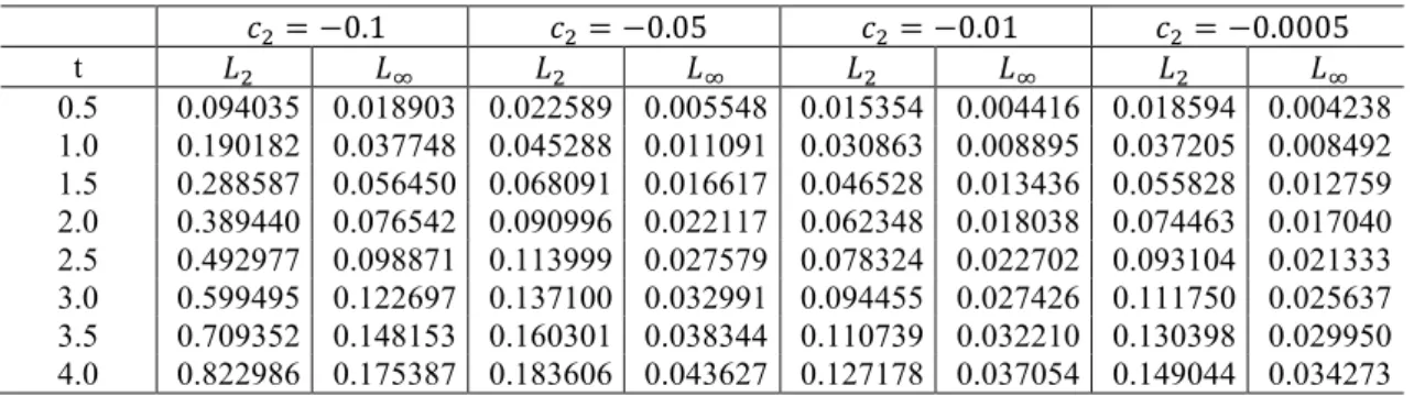
The calculated values of the error norms 𝐿# and 𝐿" are given at some chosen times up to 𝑡 = 4. The newly obtained results are tabulated in Table 6. As one can see obviously from Table 6, the error norms 𝐿# and 𝐿" have decreased when 𝑐# becomes bigger from 𝑐# = −0.1 to 𝑐# = −0.0005 values. Also, it is clearly observed from these tables that solutions by QBDQM using less number of grid points such as 𝑁 = 11 are acceptable.
Table 6. A comparison of 𝐿# and 𝐿" error norms for Δ𝑡 = 0.1, and 𝑁 = 11 at various values of 𝑐# 𝑐#= −0.1 𝑐#= −0.05 𝑐#= −0.01 𝑐#= −0.0005 t 𝐿# 𝐿" 𝐿# 𝐿" 𝐿# 𝐿" 𝐿# 𝐿" 0.5 0.094035 0.018903 0.022589 0.005548 0.015354 0.004416 0.018594 0.004238 1.0 0.190182 0.037748 0.045288 0.011091 0.030863 0.008895 0.037205 0.008492 1.5 0.288587 0.056450 0.068091 0.016617 0.046528 0.013436 0.055828 0.012759 2.0 0.389440 0.076542 0.090996 0.022117 0.062348 0.018038 0.074463 0.017040 2.5 0.492977 0.098871 0.113999 0.027579 0.078324 0.022702 0.093104 0.021333 3.0 0.599495 0.122697 0.137100 0.032991 0.094455 0.027426 0.111750 0.025637 3.5 0.709352 0.148153 0.160301 0.038344 0.110739 0.032210 0.130398 0.029950 4.0 0.822986 0.175387 0.183606 0.043627 0.127178 0.037054 0.149044 0.034273 5.4. Stability Analysis
For the proposed procedure a matrix stability analysis is made. For software, we have utilized the symbolic programming language Matrix Laboratory, that is MatLab program, for finding out the eigenvalues of the coefficient matrix . Eigenvalues of the proposed procedure for different number of grids are presented in Fig. 3. The eigenvalues for 𝑁 = 11 have only real component but for 𝑁 = 21, 𝑁 = 31, and 𝑁 = 41 have both components. It is seen that the eigenvalues are in compliance with the criteria [9].
Figure 3. Eigenvalues for various number of grid points: 𝛼 =𝛽 = 𝜆 =1
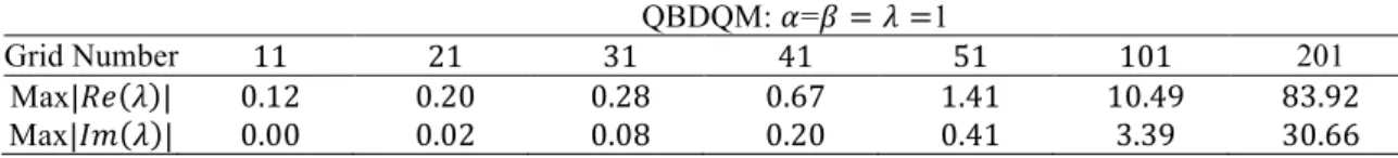
At the same time, the highest absolute value of those eigenvalues for different choices of nodes are presented in Table 7. As one can see from Table 7 when the number of the grid points increased since absolute value of eigenvalue grows, time step should be decreased to obtain the stable solution.
Table 7. The highest absolute values of the eigenvalues for different number of nodes QBDQM: 𝛼=𝛽 = 𝜆 =1
Grid Number 11 21 31 41 51 101 201
Max|𝑅𝑒 𝜆 | 0.12 0.20 0.28 0.67 1.41 10.49 83.92 Max|𝐼𝑚 𝜆 | 0.00 0.02 0.08 0.20 0.41 3.39 30.66
6. Conclusion
In the present manuscript, we have used DQM based on quintic B-splines for numerical solution of combined KdV-mKdV equation. The efficiency and accuracy of the method have been shown by calculating the error norms 𝐿# and 𝐿". One outstanding characteristics of the proposed method is its ability for obtaining better results by using less number of nodes. This may be easily seen from the tables presented in this article. As it is observed by the comparison between the presented values of the error norms 𝐿# and 𝐿" by present method and previous studies, QBDQM results are acceptable good. Stability analysis of the numerical approximation by the eigenvalues has also been made. The newly obtained results illustrate that QBDQM may be applied to find out more efficient approximate solutions of the combined KdV-mKdV equation. Thus, in conclusion, QBDQM is an accurate and efficient method to obtain the approximate solutions of several important linear and nonlinear problems.
References
[1] Wadati, M., Wave propagation in nonlinear lattice I, Journal of the Physical Soceity of Japan, 38(3), 673-680, 1975.
[2] Wadati, M., Wave propagation in nonlinear lattice II, Journal of the Physical Soceity of Japan, 38(3), 681-686, 1975.
[3] Taha, T.R., Inverse scattering transform numerical schemes for nonlinear
evolution equations and the method of lines, Applied Numerical Mathematics, 20,
181-187, 1996.
[4] Fan, E., Uniformly constructing a series of explicit exact solutions to nonlinear
equations in mathematical physics, Chaos Soliton Fract, 16, 819–39, 2003.
[5] Peng, Y., New exact solutions to the combined KdV and mKdV equation, International Journal Theoretical Physics, 42(4), 863–868, 2003.
[6] Bekir, A., On traveling wave solutions to combined KdV–mKdV equation and
modified Burgers–KdV equation, Communications in Nonlinear Science and Numerical
Simulation, 14, 1038–1042, 2009.
[7] Lu, D., Shi, Q., New solitary wave solutions for the combined KdV-MKdV
equation, Journal of Information & Computational Science, 7, 1733-1737, 2010.
[8] Bellman, R., Kashef, B. G., Casti, J., Differential quadrature: a tecnique for the
rapid solution of nonlinear differential equations, Journal of Computational Physics, Vol.
10, 40-52, 1972.
[9] Shu, C., Differential Quadrature and Its Application in Engineering, Springer-Veralg London Ltd., London, 2000.
[10] Bellman, R., Kashef, B., Lee, E.S., Vasudevan, R., Differential quadrature and
splines, Computers and Mathematics with Applications, Pergamon, Oxford, 1(3-4),
371-376, 1975.
[11] Quan, J.R., Chang, C.T., New sightings in involving distributed system
equations by the quadrature methods-I, Computers and Chemical Engineering, 13,
779-88, 1989.
[12] Quan, J.R., Chang, C.T., New sightings in involving distributed system
equations by the quadrature methods-II, Computers and Chemical Engineering, 13,
1017-1024, 1989.
[13] Shu, C., Richards, B.E., Application of generalized differential quadrature to
solve two dimensional incompressible Navier-Stokes equations, International Journal for
Numerical Methods in Fluids, 15, 791-798, 1992.
[14] Shu, C., Xue, H., Explicit computation of weighting coefficients in the
harmonic differential quadrature, Journal of Sound and Vibration, 204(3), 549-55, 1997.
[15] Zhong, H., Spline-based differential quadrature for fourth order equations and
its application to Kirchhoff plates, Applied Mathematical Modelling, 28, 353-66, 2004.
[16] Guo, Q. and Zhong, H., Non-linear vibration analysis of beams by a
spline-based differential quadrature method, Journal of Sound and Vibration, 269, 413-420,
2004.
[17] Zhong, H., Lan, M., Solution of nonlinear initial-value problems by the
spline-based differential quadrature method, Journal of Sound and Vibration, 296, 908-918,
2006.
[18] Cheng, J., Wang, B., Du, S., A theoretical analysis of piezoelectric/composite
laminate with larger-amplitude deflection effect, Part II: Hermite differential quadrature method and application, International Journal of Solids and Structures, 42, 6181-6201,
[19] Shu, C., Wu, Y.L., Integrated radial basis functions-based differential
quadrature method and its performance, The International Journal for Numerical
Methods in Fluids, 53, 969-84, 2007.
[20] Striz, A.G., Wang, X., Bert, C. W., Harmonic differential quadrature method
and applications to analysis of structural components, Acta Mechanica, 111, 85-94, 1995.
[21] Korkmaz, A., Dağ, I., Shock wave simulations using Sinc differential
quadrature method, International Journal for Computer-Aided Engineering and Software,
28(6), 654-674, 2011.
[22] Bonzani, I., Solution of non-linear evolution problems by parallelized
collocation-interpolation methods, Computers & Mathematics and Applications, 34(12),
71-79, 1997.
[23] Başhan, A., Numerical solutions of some partial differential equations with B-spline differential quadrature method, PhD, İnönü University, Malatya, 2015.
[24] Korkmaz, A., Dağ, I., Cubic B-spline differential quadrature methods for the
advection-diffusion equation, International Journal of Numerical Methods for Heat &
Fluid Flow, 22(8), 1021-1036, 2012.
[25] Korkmaz, A., Dağ, I., Numerical simulations of boundary-forced RLW
equation with cubic B-Spline-based differential quadrature methods, Arabian Journal for
Science and Engineering., 38(5), 1151-1160, 2013.
[26] Korkmaz, A., Dağ, I., Cubic B-spline differential quadrature methods and
stability for Burgers’ equation, International Journal for Computer-Aided Engineering
and Software, 30(3), 320-344, 2013.
[27] Korkmaz, A., Numerical solutions of some partial differential equations using B-spline differential quadrature methods, PhD, Eskişehir Osmangazi University, Eskişehir, 2010.
[28] Prenter, P.M., Splines and variational methods, John Wiley Publications, New York, 1975.
[29] Ketcheson, D.I., Runge–Kutta methods with minimum storage implemen-
tations, Journal of Computational Physics, 229, 1763–1773, 2010.
[30] Ketcheson, D.I., Highly efficient strong stability preserving Runge-Kutta
methods with Low-Storage Implementations, SIAM Journal on Scientific Computing,