Smart antenna systems for non-coherent source groups containing coherent signals

(Masters Thesis)

YASAR UNIVERSITY

GRADUATE SCHOOL OF NATURAL AND APPLIED SCIENCES

SMART ANTENNA SYSTEMS FOR NON-COHERENT

SOURCE GROUPS CONTAINING COHERENT

SIGNALS

Ahmad AMINU

Thesis Advisor: Asst. Prof. Dr. Mustafa SEÇMEN

Department of Electrical/Electronics Engineering

Presentation Date: 25th June, 2014

Bornova-IZMIR

YASAR UNIVERSITY

GRADUATE SCHOOL OF NATURAL AND APPLIED SCIENCES

SMART ANTENNA SYSTEMS FOR NON-COHERENT

SOURCE GROUPS CONTAINING COHERENT

SIGNALS

Ahmad AMINU

Thesis Advisor: Asst. Prof. Dr. Mustafa SEÇMEN

Department of Electrical/Electronics Engineering

Presentation Date: 25th June, 2014

Bornova-IZMIR

Approval Page

This study, titled ‘‘Smart Antenna Systems For Non-Coherent Source Groups

Containing Coherent Signals’’ and presented as Masters thesis by Ahmad AMINU, has been evaluated in compliance with the relevant provision of Y.U.

Graduate Education and Training Regulations and Y.U. Institute of Science Education and Training. The jury members below have decided for the defence of this thesis, and it has been declared by consensus / majority of votes that the candidate has succeeded in his thesis defence examination dated 25th June, 2014.

Jury Members: Signature:

Head: Asst. Prof. Dr. Mustafa SEÇMEN ...

Rapporteur Member: Asst. Prof. Dr. Nalan OZKURT ...

ABSTRACT

SMART ANTENNA SYSTEMS FOR NON-COHERENT SOURCE GROUPS CONTAINING COHERENT SIGNALS

AMINU, Ahmad

MSc. in Electrical and Electronics Engineering

Supervisor: Asst. Prof. Dr. Mustafa SEÇMEN

June 2014, 88 pages

This study presents smart antenna systems for unknown non-coherent source groups containing coherent signals. All parameters (including the frequency of each signal group) of direction-of-arrival (DOA) problem are aimed to be extracted in the presence of unknown noncoherent source groups, which are consisting of coherent signals. The antenna elements used in the fading analysis and application are isotropic, linear and uniformly distributed, and all parameters of the complete signal are assumed to be unknown except the number of coherent signal in each noncoherent group.

To obtain the desired parameters (number of noncoherent groups, arrival angles, fading coefficients, frequencies), a four-step approach are followed. First, the number of noncoherent signal groups is determined by the minimum description length (MDL). Then, effective steering vectors are estimated using the joint approximate diagonalization of eigenmatrices (JADE) algorithm. In the third step, by using these steering vectors some popular high-resolution DOA methods such as the modified forward backward linear prediction (MFBLP), estimation of signal parameters via rotational invariance techniques (ESPRIT), multiple signal classification (MUSIC), and Minimum-norm (Min-norm) algorithms are realized to calculate the arrival angle and fading coefficient of each coherent signal. Afterwards, a frequency matching is realized to assign the possible frequency to each group.

Root mean square error (RMSE) values for DOAs and fading coefficients are computed in a very challenging case having extreme fading coefficients for all

the methods used and the corresponding results are compared for different scenarios such as different SNR, different number of antenna elements and snapshots. Although all the methods resolved the signals correctly, simulation results show that JADE based MFBLP has the superior performance.

The DOAs obtained from the JADE-MFBLP are then processed using steepest descent, least mean square (LMS) and normalized LMS adaptive beamforming algorithms to steer the main lobe of the radiation pattern to desired angles (signals) and the nulls to undesired angles (signals). The simulation results also reveal that adaptive beamforming is successfully done by cancelling the effects of undesired signals significantly. Finally, the reduction of power in dB for the worst case where all undesired signals are out of phase to the desired signal is investigated. The simulation results present that in spite of challenging environment with strong fading coefficients, the algorithms are able to make a successful beamform adaptively such that the power reduction is observed as 5.80 dB, 1.04dB and 2.86 dB at most for SD, LMS and NLMS respectively.

Keywords: adaptive beamforming, direction of arrival (DOA), estimation of signal parameters via rotational invariance techniques (ESPRIT), fading, joint approximate diagonalization of eigenmatrices (JADE), least mean square (LMS) algorithm, minimum description length (MDL), minimum-norm (Min-norm), modified forward backward linear prediction (MFBL), multiple signal classification (MUSIC)

ÖZET

Bu çalışma, uyumlu sinyaller içeren bilinmeyen uyumlu olmayan kaynak grupları için akıllı anten sistemlerini sunmaktadır. Geliş yönü probleminin tüm parametreleri (her sinyal grubunun frekansını içeren) uyumlu sinyallerden oluşan bilinmeyen uyumlu olmayan kaynak grupları varlığında ayıklanması amaçlanmıştır. Sönümleme analizinde kullanılan anten elemanları izotropiktir, doğrusal ve düzgün dağılımlıdır ve sinyalin tüm parametreleri her uyumlu olmayan gruptaki uyumlu sinyal sayısı dışında bilinmiyor varsayılmıştır.

İstenilen parametreleri (uyumlu olmayan grup sayısı, geliş açısı, zayıflama katsayıları, frekanslar) elde etmek için dört aşamalı yaklaşım izlenmiştir. İlk olarak, uyumlu olmayan sinyal gruplarının sayısı minimum tanımlama uzunluğu ile belirlenmiştir. Sonra, öz ortak yaklaşık köşegenleştirme algoritması kullanılarak etkili yönelimvektörleri kestirilmiştir. Üçüncü aşamada ise bu yönelim vektörleri; modifiye edilmiş ileri geri lineer tahmin (MFBLP), rotasyonel değişmezlik tekniği ile sinyal parametrelerinin kestirimi (ESPRIT), çoklu sinyal sınıflandırma (MUSIC), temel çoklu sinyal sınıflandırma (root-MUSIC) ve minimum norm (Min-norm) algoritmaları gibi bazı yüksek çözünürlükte DOA metodları kullanılarak açı ve her uyumlu sinyalin zayıflama katsayısının hesaplama işlemi gerçekleştirilmiştir. Ardından her gruba frekans atamak için frekans eşleştirme yapılmıştır.

Her metod kullanılarak DOA’lar için ortalama hata kareleri toplamı kökü (RMSE) ve zayıflama katsayıları için bağıl RMSE değerleri farklı senaryolarda hesaplandı ve karşılaştırma yapıldı. Tüm metodlar sinyali doğru çözümlemesine rağmen simülasyon sonuçları JADE tabanlı MFBLP yönetmin en iyi performansa sahip olduğunu gösterdi.

Jade-MFBLP’den elde edilen DOA’lar, radyasyon paterninin ana lobunu istenilen açıya yönlendirmek için ve istenmeyen açılarda sıfıra denk gelmesi içindik iniş, en küçük karesel ortalama (LMS) ve normalize LMS adaptif hüzme şekillendirme algoritmaları kullanılarak işleme konuldu. Simülasyon sonuçları, adaptif hüzme şekillendirici yönteminin istenmeyen sinyal etkilerini yok etmede başarılı olduğunu gösterdi. Son olarak, tüm istenmeyen sinyallerin istenen sinyale göre faz dışında kalması en kötü durum olarak kabul edildi ve bu durumda sinyaldeki düşüş dB cinsinden incelendi. Simülasyon sonuçları, güçlü zayıflama katsayılı zorlu çevre şartlarına rağmen, algoritmaların adaptif olarak başarılı hüzme yapabildiğini gösterdi. Örneğin M=12 ve M=500 enstantenesinde LMS,

NLMS ve dik iniş algoritmaları ile alınan güç azalma sonuçları sırasıyla 1.04 dB, 2.86dB ve 5.80dB olduğu gözlemlendi.

Anahtar Kelimeler: adaptif hüzme şekillendirme, varış açısı, rotasyonel

değişmezlik tekniği yöntemiyle sinyal parametrelerinin kestirimi, zayıflama, özmatrislerin birleşik yakın köşegenleştirilmesi, en küçük karesel ortamala algoritması, minimum tanımlayıcı uzunluk, minimum norm, modifiye edilmiş ileri geri lineer tahmin, çoklu sinyal sınıflandırma, normalize en küçük karesel ortalama algoritması, temel çoklu sinyal sınıflandırma

ACKNOWLEDGEMENTS

First, I would like to thank Allah subhaanahuu wa ta’ala for the knowledge and strength that made this research work possible. I would like also to thank my supervisor Asst. Prof. Dr. Mustafa Seçmen for his tireless contribution, guidance and patience during this study. In addition, I would like to thank the jury members and also staff of Electrical and Electronics Engineering department, Yasar University, for their support and encouragement towards the successful completion of this thesis and indeed the MSc program.

I would also like to express my sincere gratitude to my wife especially for her patience and encouragement, my children, rest of the family and friends here in Turkey and also those in Nigeria for their well wishes. I thank you very much.

Finally, my profound gratitude goes to His Excellency, the executive governor of Kano state, Engr. (Dr.) Rabi’u Musa Kwankwaso and his cabinet for the scholarship awarded to me to undergo this postgraduate program here at Yasar University, Izmir Turkey.

TEXT OF OATH

I declare and honestly confirm that my study, titled ‘‘Smart Antenna Systems

For Non-Coherent Source Groups Containing Coherent Signals’’ and

presented as a Master’s thesis, has been written without applying to any assistance inconsistence with scientific ethics and traditions, that all sources from which I have benefited are listed in the bibliography, and that I have benefited from these sources by means of making references.

Date: 25th June, 2014

Ahmad AMINU

TABLE OF CONTENT Pages ABSTRACT ... iv ÖZET ... vi ACKNOWLEDGEMENTS ... viii TABLE OF CONTENT ... x

INDEX OF FIGURES ... xiii

INDEX OF TABLES ... xvi

1. INTRODUCTION ... 1

1.1 Background of the Study ... 1

1.2 Scope of the Thesis ... 3

1.3 Aim of the Study ... 3

1.4 Methodology of the Study... 3

1.5 Thesis Outline ... 4

2. THE OVERVIEW OF SMART ANTENNA SYSTEMS... 5

2.1 Antenna ... 5

2.1.1 Omni directional Antenna ... 5

2.1.2 Directional Antenna ... 7

2.2 Smart Antenna ... 8

2.3 Types of Smart Antenna ... ..11

2.3.1 Adaptive Array ... 11

2.3.2 Switched Beam...11

2.4 Working principles of Smart Antenna systems...12

2.4.1 Listening to the Cell (Uplink Processing)...12

2.4.2 Speaking to the Users (Downlink Processing...13

2.5 Advantages and Disadvantages of Smart Antenna...13

2.5.1 Advantages...13

2.5.2 Disadvantages...15

3. SIGNAL MODEL AND STEPS OF THE PROPOSED METHOD FOR DOA ESTIMATION...16

3.1 Array Model For Non coherent Source Groups Containing Coherent Signals...16

3.2 MDL Algorithm...19

3.3 Steering Vector Estimation Using JADE Algorithm...19

3.4 DOA Estimation Algorithms...20

3.4.1 Multiple Signal Classification (MUSIC) Algorithm...20

3.4.2 Minimum norm Algorithm...21

3.4.3 Root-MUSIC Algorithm...21

3.4.4 Estimation of Signal Parameters via Rotational Invariance Technique (ESPRIT) Algorithm...22

3.4.5 Modified Forward Backward Linear Prediction (MFBLP) Algorithm.22 3.5 Fading Coefficient Estimation...24

3.6 Frequency Matching...25

4. SIMULATION RESULTS FOR DOA AND FADING COEFFICIENTS WITH FREQUENCY MATCHING...27

4.1 Simulation of DOA Estimation algorithms...27

4.2 Performance Comparison of DOAs and Fading coefficients...33

4.3 Comparison of Computation Time...37

4.4 Analysis of Frequency Matching Result...38

5. BEAMFORMING...40

5.1 Beamforming Algorithms...40

5.1.1 Steepest Descent...40

5.1.2 Least Mean Square Algorithm...41

5.1.3 Normalized Least Mean Square Algorithm...42

5.2 The Measure for Performance Evaluation of Beamforming Algorithms...43

6. SIMULATIONS and RESULTS for BEAMFORMING... 45

6.1 Adaptive Beamforming Simulation Results...45

6.1.1 Steepest Descent Algorithm Simulation Result...46

6.1.2 Least Mean Square Algorithm Simulation Result...49

6.1.3 Normalized Least Mean Square Algorithm Simulation Result...52

6.2 Some Factors Affecting Beam formation...55

6.2.1 Effect of number of array elements on beam formation...55

6.2.2 Effect of elements inter-spacing on beam formation...58

6.3 Comparison of Steepest Descent, LMS and Normalized LMS in terms of Signal Power Reduction and Computation Time...60

7.1 Conclusions...62

7.2 Future Work...63

BIBLIOGRAPHY...64

INDEX OF FIGURE

FIGURE PAGE

2.1 Omni directional Antenna and Coverage Patterns ... 6

2.2 Active Directional Antenna and Coverage Pattern ... 7

2.3a Human Analogy ... 8

2.3b Electrical Equivalent ... 9

2.4 A Sample Smart Antenna System ... 10

2.5 Adaptive Array System, Representative Depiction of a Main Lobe Extending Toward a User ... 11

2.6 Switched Beam System ... 12

3.1 Uniform Linear Array with M elements ... 16

4.1 The estimation of Min-norm spectrum for (a) the first signal group (b) the second signal group (c) the third signal group, for 50 Monte-Carlo trials. The high peaks indicate the estimated DOAs of the signals. ... 30

4.2 The estimation of MUSIC spectrum for (a) the first signal group (b) the second signal group (c) the third signal group, for 50 Monte-Carlo trials. The high peaks indicate the estimated DOAs of the signals. ... 31

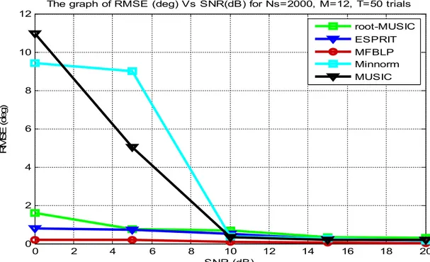
4.3 RMSE versus different SNR values for root-MUSIC, ESPRIT, MFBLP Min-norm and MUSIC algorithms ... 33

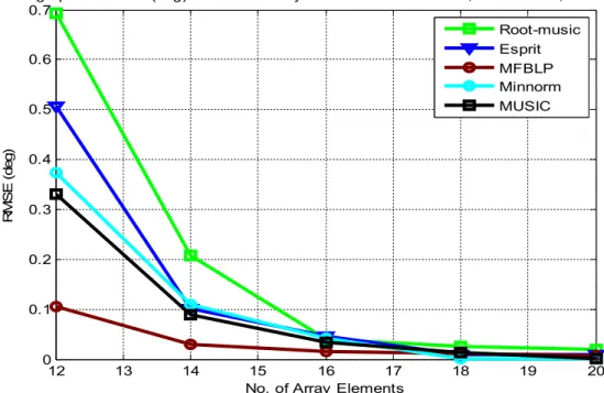
4.4 RMSE versus different Number of Array Elements values for root-MUSIC, ESPRIT, MFBLP Min-norm and MUSIC algorithms. ... 34

4.5 RMSE versus different Number of snapshots values for root-MUSIC, ESPRIT, MFBLP Min-norm and MUSIC algorithms ... 35

4.6 RMSE for fading coefficients versus different SNR values for root-MUSIC, ESPRIT, MFBLP Min-norm and MUSIC algorithms ... 36

4.7 7 RMSE for fading coefficients versus different Number of Array Elements values for root-MUSIC, ESPRIT, MFBLP Min-norm and MUSIC algorithms ... 36

4.8 RMSE for fading coefficients versus different Number of snapshots values for root-MUSIC, ESPRIT, MFBLP Min-norm and MUSIC algorithms. .... 37

4.9 Percentages of “correct” matching versus different SNR levels for root-MUSIC, ESPRIT and MFBLP algorithms ... 39

6.1 Radiation pattern of the adaptive beamforming using Steepest Descent algorithm for (a) the first signal group (b) the second signal group (c) the third signal group ... 47

6.2 Array factor verses Angle of Arrival for (a) the first signal group (b) the second signal group (c) the third signal group using Steepest Descent algorithm ... 48

6.3 Radiation pattern of the adaptive beamforming using LMS algorithm for (a) the first group (b) the second group (c) the third signal group ... 50

6.4 Array factor verses Angle of Arrival for (a) the first signal group (b) the second signal group (c) the third signal group using LMS algorithm ... 52

6.5 Radiation pattern of the adaptive beamforming for (a) the first group (b) the second group (c) the third signal group using NLMS algorithm ... 53

6.6 Array factor verses Angle of Arrival for (a) the first signal group (b) the second signal group (c) the third signal group using NLMS algorithm ... 55

6.7 Impact of number of number of elements on radiation pattern for (a) M=12, (b) M=20, using LMS algorithm ... 56

6.8 Impact of number of number of elements on radiation pattern for (a) M=12, (b) M=20, using NLMS algorithm ... 57

6.9 Impact of element spacing on radiation pattern for (a) d=0.5λ and (b) d= λ, using LMS algorithm. ... 59

6.10 Impact of element spacing on radiation pattern for (a) d=0.5λ and (b) d= λ, using NLMS algorithm. ... 60

INDEX OF TABLE

TABLE PAGE

4.1 True values of DOAs and Fading coefficients... ………..28

4.2 True Arrival Angle and Mean of estimated DOA Angles... ………..28

4.3 Computation Time comparisons ... 37

4.4 Variation of Number of correct freq. matching with SNR ... 38

5.1 Estimated fading coefficients ... 44

6.1 Estimated values of DOAs and Fading coefficients using MFBLP... 45

6.2 Comparison of Steepest descent, LMS and NLMS algorithms in terms of Signal Power Reduction (dB) ... 61

6.3 Comparison of Steepest descent, LMS and NLMS algorithms in terms of Computation time (sec) ... 61

1. INTRODUCTION

1.1 Background of the Study

Wireless Communication is growing with a very rapid rate for several years. The progress in radio technology enables new and improved services. Current wireless services include transmission of voice, fax and low-speed data. More bandwidth consuming interactive multimedia services like video-on demand and internet access are supported.

Wireless systems that enable higher data rates and higher capacities have become the need of the present time (Khumane et al., 2011). At the same time, operators want to support more users per base station in order to reduce overall network cost and make the services affordable to subscribers. Wireless networks must provide these services in a wide range of environments, dense urban, suburban, and rural areas. Because the available broadcast spectrum is limited, attempts to increase traffic within a fixed bandwidth create more interference in the system and degrade the signal quality (Tsoulos, 1999).

The solution to this problem is “SMART ANTENNA”. Today's modern wireless mobile communications depend on adaptive "smart" antennas to provide maximum range and clarity. With the recent explosive growth of wireless applications, smart antenna technology has achieved widespread commercial and military applications (Tsoulos et al., 1995)

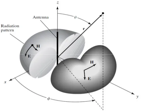
Any smart antenna system merges an antenna array and a signal processing unit to combine the incident signals on the array adaptively through weight adjustment. The signal processing consists of direction of arrival (DOA) estimation and adaptive beamforming part. Various methods for DOA estimation and beamforming are available, which differ in accuracy, computational complexity and convergence speed. The appropriate algorithm for DOA estimation or beamforming may differ from one application to another. DOA estimation is an important problem in array signal processing. Angle estimation may be used for source localization or source tracking by determining the desired signal location or may be exploited to reduce the unwanted effects of noise and interference. Therefore, DOA estimation, Angle of Arrival (AOA) or Time of Arrival (TOA) estimation is applicable in various fields such as radar, sonar, navigation, geophysics, wireless communications and so on (Balanis, 2005),

(Chen et al., 2010). In adaptive array antennas or smart antenna systems, DOA estimation algorithms provide information about the system environment for an efficient beamforming or providing location-based services such as emergency services. Therefore, great researches have been accomplished about DOA estimation during recent years, including different methods, different signal and system conditions, different array geometries and applications (Okamoto, 2002), (Balanis, 2005).

The studies described above and traditional theory of DOA estimation are based on the sources (or signals) which are uncorrelated (noncoherent) to each other. These noncoherent signals can be considered as multiple users or frequencies in the wireless communication applications. The estimation of DOA angles for these types of signals are relatively easier and classical DOA estimation can be safely applied for this purpose. Then, the beamforming algorithms can be carried out to get maximum signal from one user and minimum signals from other users which can be treated as interference signals. However, since the frequencies of different users are different due to noncoherent behaviours of the signals, the effective cancellation of undesired signals (users) can be realized by putting suitable narrow passband filters even beamforming techniques are not used. On the other hand, more difficult and challenging scenario is observed when the desired and undesired signals are coherent (correlated) such as multipath signals. Multipath or fading signals are time-shifted replicas of the original desired signals (usually coming from different incident angles than that of original desired signal); so their frequencies are same as the desired signals. Therefore, they could not be annihilated by using filter approach. These multipath signals have very adverse effects such as total cancellation of the desired signal. Therefore, the reducing the effect of multipath signals of the same user is much more important than the decreasing the signal levels of other users (different frequencies). The difficulty in DOA estimation under multipath propagation is that since the desired and undesired fading signals are coherent, the classical DOA estimation algorithms cannot be directly used, and more intelligent methods should be used.

With these intelligent methods, smart antennas combining DOA estimation under coherent signal environment and corresponding beamforming can improve the system performance by helping the channel modelling and suppression undesirable signals like multipath fading and co-channel interference (Varade et al., 2009).

1.2 Scope of the Thesis

By regarding to the difficulties explained above for the smart antenna systems for signals with multipath effect, the scope of this thesis is limited to simulation of different DOA and fading coefficients estimation algorithms in multipath propagation, frequency matching and adaptive beamforming with a view to implement smart antenna system for wireless and mobile communication systems. For this purpose, several DOA estimation algorithms such as ESPRIT, MUSIC, root-MUSIC Min-norm and MFBLP in conjunction with JADE are realized to estimate the DOAs of different coherent signals (multipath environment) and then steepest descent, LMS and NLMS beamforming algorithms are used to adjust the complex weights and to generate an optimized radiation pattern with mainlobes and nulls in the direction of desired and undesired signals, respectively.

1.3 Aim of the Study

This study aimed at implementing Smart Antenna System especially for high frequency and non-coherent source groups each having coherent signals. The excitation coefficients of the antenna array elements are going to be optimized to maximize the main lobes toward the signal-of-interest (SOI) angles and nulls toward the signal-not-of-interest (SNOI) angles. For this purpose several direction-of-arrival algorithms and beam forming algorithms are realized to obtain a sufficient method even under noisy signal conditions. The study also aimed at estimating and correctly matching different frequencies to different non-coherent source groups and this will be the main contribution of this thesis to the literature of direction of arrival (DOA) estimation.

1.4 Methodology of the Study

In the first stage of the thesis, minimum description length (MDL) is used to determine the number of non-coherent source groups and then, joint approximate diagonalization of eigenmatrices (JADE) algorithm is used to estimate the generalized steering vectors.DOA parameters such as angles of arrival and fading coefficients are estimated by using several high resolution methods such as ESPRIT, MUSIC, ROOT-MUSIC, MFBLP and Min-norm and their results are compared. Frequency matching to non-coherent signal groups is also done in this stage.

The second stage involves using steepest descent, LMS and normalized LMS algorithms for beam forming to steer the main lobes of the array toward the signals-of interest (SOI) and nulls to the signals-not-of-interest (SNOI).

1.5 Thesis Outline

The report of the thesis is outline as follows. Chapter 2 contains the background knowledge of antenna and antenna systems, types of antenna, smart antenna systems and its types, advantages and disadvantages.

In chapter 3, the signal model, DOAs and fading coefficients estimation algorithms are discussed. The concept of frequency or group matching is also introduced in this chapter.

Chapter 4 includes the simulation results for DOA and fading coefficients, frequency/group matching result as well as comparative analysis results of different types of DOA and fading coefficients estimation algorithms.

The adaptive beamforming algorithms such as steepest descent, least mean square (LMS) and normalized LMS are discussed in chapter 5.

Chapter 6 discusses the simulation results of steepest descent, LMS and NLMS, in addition to the effect of changing the number of antenna elements and spacing between elements on the beamforming and on the mean square error. Finally, the effect of step-size on the beamforming and on the convergence speed of the two beamforming algorithms was investigated also in this chapter.

2. THE OVERVIEW OF SMART ANTENNA SYSTEMS

In this chapter, the concept of antenna, direction of arrival and smart antenna systems are presented to give an insight and better understanding of the contents of the thesis.

2.1 Antenna

An antenna (or aerial) is a transducer designed to transmit or receive electromagnetic waves. In other words, antennas convert electromagnetic waves into electrical currents and vice versa. Antennas are used in systems such as radio and television broadcasting, point-to-point radio communication, wireless LAN, radar, and space exploration. Antennas are most commonly employed in air or outer space, but can also be operated under water or even through soil and rock at certain frequencies for short distances (Okamoto, 2006).

Physically, an antenna is simply an arrangement of one or more conductors, usually called elements. In transmission, an alternating current is created in the elements by applying a voltage at the antenna terminals, causing the elements to radiate an electromagnetic field. In reception, the inverse occurs such that an electromagnetic field from another source induces an alternating current in the elements and a corresponding voltage at the antenna's terminals. Some receiving antennas (such as parabolic types) incorporate shaped reflective surfaces to collect EM waves from free space and direct or focus them onto the actual conductive elements.

There are two fundamental types of antenna directional patterns, which, with reference to a specific three dimensional (usually horizontal or vertical) plane are either:

 Omni-directional (radiates equally in all directions), such as a vertical rod.  Directional (radiates more in one direction than in the other).

2.1.1 Omni directional Antenna

Omni-directional usually refers to all horizontal directions with reception above and below the antenna being reduced in favour of better reception (and thus range) near the horizon.

Since the early days of wireless communications, there has been the simple dipole antenna, which radiates and receives equally well in all directions. To find its users, this single-element design broadcasts omnidirectionally in a pattern resembling ripples radiating outward in a pool of water as shown in Fig. 2.1 below. While adequate for simple RF environments where no specific knowledge of the users' whereabouts is available, this unfocused approach scatters signals, reaching desired users with only a small percentage of the overall energy sent out into the environment.

Figure 2.1: Omni-directional Antenna pattern (Balanis, 2005)

With this limitation, omnidirectional strategies attempt to overcome environmental challenges by simply boosting the power level of the signals broadcast. In a setting of numerous users (and interferers), this makes a bad situation worse in that the signals that miss the intended user become interference for those in the same or adjoining cells.

In uplink applications (user to base station), Omni directional antennas offer no preferential gain for the signals of served users. In other words, users have to shout over competing signal energy. Also, this single-element approach cannot selectively reject signals interfering with those of served users and has no spatial multipath mitigation or equalization capabilities.

Omni directional strategies directly and adversely impact spectral efficiency, limiting frequency reuse. These limitations force system designers and network planners to devise increasingly sophisticated and costly remedies. In recent years, the limitations of broadcast antenna technology on the quality, capacity, and coverage of wireless systems have prompted an evolution in the fundamental design and role of the antenna in a wireless system.

2.1.2 Directional Antenna

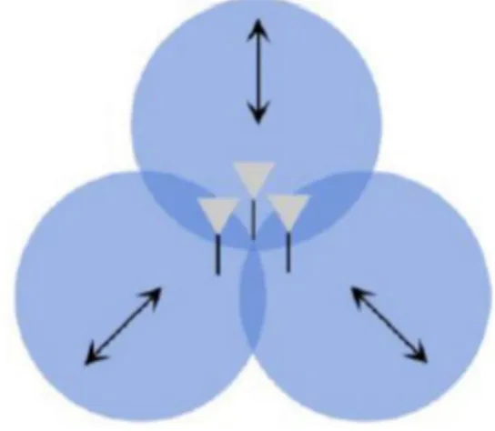
A "directional" antenna usually refers to one focusing a narrow beam in a single specific direction as shown in Fig. 2.2 below. A single antenna can also be constructed to have certain fixed preferential transmission and reception directions. As an alternative to the brute force method of adding new transmitter sites, many conventional antenna towers today split, or sectorized cells. A 360° area is often split into three 120° subdivisions, each of which is covered by a slightly less broadcast method of transmission.

All else being equal, sector antennas provide increased gain over a restricted range of azimuths as compared to an omnidirectional antenna. This is commonly referred to as antenna element gain and should not be confused with the processing gains associated with smart antenna systems.

Figure 2.2: Directional Antenna Pattern (Jain, 2011)

While sectorized antennas multiply the use of channels, they do not overcome the major disadvantages of standard omnidirectional antenna broadcast such as co-channel interference.

All antennas radiate some energy in all directions in free space but careful construction results in substantial transmission of energy in a preferred direction and negligible energy radiated in other directions.

Smart antenna systems normally use more than one antenna elements; consequently, even if the antenna elements are omnidirectional, the overall array structure is directional. The main aim of the smart antenna systems is to direct the mainbeam of the radiation pattern of the array towards the desired signal and put nulls at the angles of undesired ones in the radiation pattern. The traditional phased antenna array technology (Balanis, 2005) can direct the main beam of the radiation pattern of the array to the desired signal’s angle of arrival once DOA angle of the desired signal is estimated. However, it does not care about the positioning of nulls at the undesired signals’ DOA angles. Therefore, it is not evaluated as a smart antenna system. On the other hand, some null insertion antenna methods such as Schelkunoff polynomial method (Balanis, 2005) can successfully put nulls at the DOA angles of undesired signals in the radiation pattern. Nevertheless, they have no abilities to maximize the level of desired signal such that the main beam of the array is usually not directed to the DOA of desired angle, and even DOA of desired signal may corresponds to the null in the pattern.

2.2 Smart Antennas

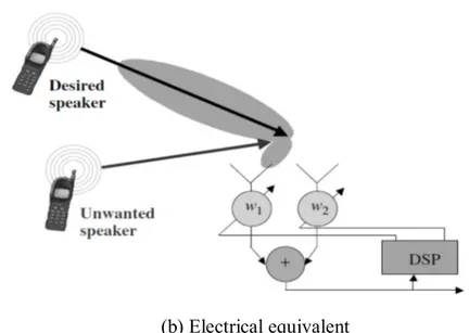
The smart antenna systems can be understood better when its working principles are compared with human body (Balanis, 2005). Figure 2.3 below depicts the human analogy as well as the electrical equivalent of smart antenna systems.

`

(b) Electrical equivalent

Figure 2.3 Smart Antenna Analogy (a) Human analogy (Balanis, 2005); (b) Electrical equivalent

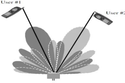
Therefore, to give an insight into how a smart-antenna system works, let us imagine two persons carrying on a conversation inside a dark room (Balanis, 2005)

[refer to Figure 2.3(a)]. The listener among the two persons is capable of determining the location of the speaker as he moves about the room because the voice of the speaker arrives at each acoustic sensor, the ear, at a different time. The human signal processor, the brain, computes the direction of the speaker from the time differences or delays of the voice received by the two ears. Afterward, the brain adds the strength of the signals from each ear so as to focus on the sound of the computed direction. Furthermore, if additional speakers join in the conversation, the brain can tune out unwanted interferers and concentrate on one conversation at a time (Balanis, 2005). Conversely, the listener can respond back to the same direction of the desired speaker by orienting the transmitter (mouth) toward the speaker.

Electrical smart-antenna systems work the same way using two antennas instead of the two ears and a digital signal processor instead of a brain(Balanis, 2005) [refer to Figure 2.3(b)]. Therefore, after the digital signal processor measures the time delays from each antenna element, it computes the direction of arrival (DOA) of the signal-of-interest (SOI), and then it adjusts the excitations (gains and phases of the signals) to produce a radiation pattern that focuses on the SOI while, ideally, tuning out any signal-not-of interest (SNOI) (Balanis, 2005).

Contrary to the name smart antennas consist of more than an antenna. A smart antenna is an antenna system, which dynamically reacts to its environment to provide better signals and frequency usage for wireless communications. There are a variety of smart antennas which utilize different methods to provide improvements in various wireless applications.

The concept of using multiple antennas and innovative signal processing to serve cells more intelligently has existed for many years. In fact, varying degrees of relatively costly smart antenna systems have already been applied in defence systems. Until recent years, cost barriers have prevented their use in commercial systems (Balanis, 2005). The advent of powerful low-cost digital signal processors (DSPs) and general-purpose processors, as well as innovative software-based signal-processing techniques (algorithms) have made intelligent antennas practical for cellular communications systems (Balanis, 2005).

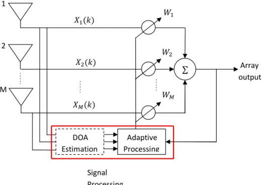
Figure 2.4: A Sample Smart Antenna System (Moghaddam, 2012)

Today, when spectrally efficient solutions are increasingly a business imperative, these systems are providing greater coverage area for each cell site, higher rejection of interference, and substantial capacity improvements. Figure 2.4 above shows the general block diagram of a sample smart antenna system.

Array output 1 2 M ( ) ( ) ( ) DOA Estimation Adaptive Processing Signal Processing ∑

2.3 Types of Smart Antenna

The two major categories of smart antennas regarding the choices in transmit strategy are Adaptive and Switch beam.

2.3.1 Adaptive Array

Adaptive antennas which consist of an infinite number of patterns (scenario-based) that are adjusted in real time represents the most advanced smart antenna approach to date (Tsoulos et al., 1995).Using variety of available signal processing algorithms, the adaptive system takes advantage of its ability to effectively locate and track various types of signals to dynamically minimize interference and maximize intended signal reception as shown in Figure2.5 below.

Figure 2.5: Adaptive Array System, Representative Depiction of a Main Lobes Extending Toward desired Users (Balanis, 2005)

2.3.2 Switched Beam

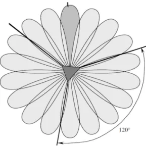
Switched beam antenna systems which consist of finite number of fixed, predefined patterns or combining strategies (sectors) form multiple fixed beams as shown in Figure 2.6 below, with heightened sensitivity in a particular direction. These antenna systems detect signal strength, choose from one of several predetermined, fixed beams, and switch from one beam to another as the mobile moves throughout the sector (Khumane et al., 2011).

Figure 2.6: Switched beam system (Balanis, 2005)

Instead of shaping the directional antenna pattern with the metallic properties and physical design of a single element (like a sectorized antenna), switched beam systems combine the outputs of multiple antennas in such a way as to form finely sectorized (directional) beams with more spatial selectivity than can be achieved with conventional approaches.

The task of transmitting in a spatially selective manner is the major basis for differentiating between switched beam and adaptive array systems. As described above, switched beam systems communicate with users by changing between preset directional patterns, largely on the basis of signal strength. In comparison, adaptive arrays attempt to understand the RF environment more comprehensively and transmit more selectively. Both systems attempt to increase gain according to the location of the user, however, only the adaptive system provides optimal gain while simultaneously identifying, tracking, and minimizing interfering signals.

2.4 WorkingPrinciples of Smart AntennaSystems

Adaptive array and switched beam systems enable a base station to customize the beams they generate for each remote user effectively by means of internal feedback control. Generally speaking, each of the two approaches forms a main lobe toward individual users and attempts to reject interference or noise from outside of the main lobe.

2.4.1 Listening to the Cell (Uplink Processing)

It is assumed here that a smart antenna is only employed at the base station and not at the handset or subscriber unit. Such remote radio terminals transmit using omnidirectional antennas, leaving it to the base station to separate the desired signals from interference selectively. Typically, the received signal from the spatially distributed antenna elements is multiplied by a weight, a complex adjustment of amplitude and a phase. These signals are combined to yield the array output. An adaptive algorithm controls the weights according to predefined objectives. For a switched beam system, this may be primarily maximum gain; for an adaptive array system, other factors may receive equal consideration. These dynamic calculations enable the system to change its radiation pattern for optimized signal reception.

2.4.2 Speaking to the Users (Downlink Processing)

The type of downlink processing used depends on whether the communication system uses time division duplex (TDD), which transmits and receives on the same frequency (e.g., PHS and DECT) or frequency division duplex (FDD), which uses separate frequencies for transmit and receiving (e.g., GSM). In most FDD systems, the uplink and downlink fading and other propagation characteristics may be considered independent, whereas in TDD systems the uplink and downlink channels can be considered reciprocal. Hence, in TDD systems uplink channel information may be used to achieve spatially selective transmission. In FDD systems, the uplink channel information cannot be used directly and other types of downlink processing must be considered.

2.5 Advantages and Disadvantages of Smart Antennas

2.5.1 Advantages

 Increased Number of Users

Due to the targeted nature of smart antennas, frequencies can be reused allowing an increased number of users. More users on the same frequency space means that the network provider has lower operating costs in terms of purchasing frequency space.

 Increased Range

As the smart antenna focuses gain on the communicating device, the range of operation increases. This allows the area serviced by a smart antenna to increase. This can provide a cost saving to network providers as they will not require as many antennas/base stations to provide coverage.

 Geographic Information

As smart antennas use ‘targeted’ signals the direction in which the antenna is transmitting and the gain required to communicate with a device can be used to determine the location of a device relatively accurately. This allows network providers to offer new services to devices. Some services include, guiding emergency services to locations, location based games and locality information.

 Security

Smart antennas naturally provide increased security, as the signals are not radiated in all directions as in a traditional omni-directional antenna. This means that if someone wished to intercept transmissions they would need to be at the same location or between the two communicating devices.

 Reduced Interference

Interference which is usually caused by transmissions which radiate in all directions is less likely to occur due to the directionality introduced by the smart antenna. This aids both the ability to reuse frequencies and achieve greater range.

 Increased bandwidth

The bandwidth available increases form the reuse of frequencies and also in adaptive arrays as they can utilize the many paths which a signal may follow to reach a device.

2.5.2 Disadvantages

 Complex

One of the disadvantages of smart antennas is that, they are far more complicated than traditional antennas. This means that faults or problems are more likely to occur and harder to be diagnosed.

 More Expensive

As smart antennas are extremely complex, utilizing the latest in processing technology they are far more expensive than traditional antennas. However, this cost must be weighed against the cost of frequency space.

 Larger Size

Due to the antenna arrays which are utilized by smart antenna systems, they are much larger in size than traditional systems. This can be a problem in a social context as antennas can be seen as ugly or unsightly.

3. SIGNAL MODEL AND THE STEPS OF PROPOSED METHOD FOR DOA ESTIMATION

In this chapter, the data model for the overall signal on the antenna elements and problem geometry will be given. The steps of the DOA estimation part of the study are discussed in detail by including DOA estimation algorithms, fading coefficients estimation and frequency matching for noncoherent source groups containing coherent signals. The similar methods in literature, which use same signal model, are also described in the chapter, and their drawbacks are going to be explained.

3.1 Array Model for Noncoherent Source Groups Containing Coherent Signals

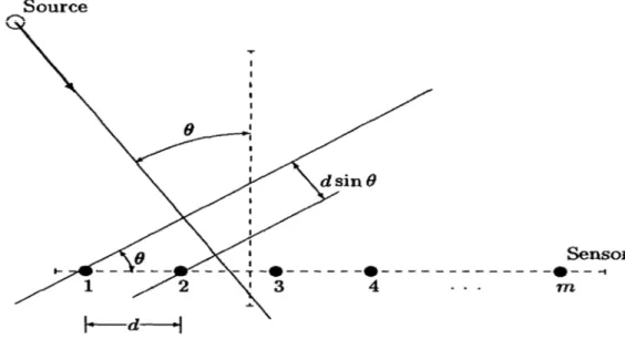
In the array model of the problem, it is assumed that there are N narrowband signals arriving to the array in the directions {θ1, θ2, θ3, . . . ,θN}. In order to simplify the problem under consideration, a uniform linear array (ULA) shown in Figure 3.1 below is assumed with inter-element spacing d of half wavelength of the narrowband signal frequency. In the mentioned figure, only one plane wave being incident in the direction θ is depicted for simplicity such that total of N plane waves actually exists in the system. M antenna elements in the array of Figure 3.1 have identical isotropic responses, and “the reference point” of the system is taken as the leftmost antenna element in the array.

Figure 3.1: Uniform Linear Array with M Antenna Elements Where a Sample Plane Wave Impinges upon the Array at the Direction of Arrival of θ.

In the model, K different RF or down converted IF frequencies {ω1,

ω2,…,ωK} are used to denote the number of different users in wireless communication. At each frequency (group), there are L coherent signals (assumed to be known) where K×L is equal to N. All parameters of the complete signal are assumed to be unknown except the number of coherent signal in each noncoherent group.

Data received at antenna elements can be described by an M × 1 vector as:

 

 

 

X As n _(3.1)

where Ns is the number of snapshots and A is the array steering matrix which is described for uniform linear array as:

 

 

 

a



a



a







 



A



 

[1





]

a





e



e

where d and λ are antenna inter-element spacing and signal wavelength, respectively. In equation (3.1), s is a vector of signals including the fading coefficients of the signals such that

 

s

k





_



e



e



e



e



_









whereρ1,…,ρN are complex fading coefficients of the signals. Here, the signals and correspondent fading coefficients from n = 1,…,L belongs to first group (frequency), and the fading coefficients from n = N-L+1,…, N belongs to signals in last group. The n in (3.1) is a vector of additive white Gaussian noise. It is assumed that the entries of s(k) and n(k) are zero mean processes and the entries of n(k) are independent with each other and signals.

Researchers in the area of signal processing have been working for decades to try to resolve highly correlated signals, which are resulted due to multipath and fading phenomena as described above. Coherent signals cause covariance matrix to be singular with rank loss and zero determinant which means the signals cannot be directly resolved using second order statistics base subspace methods. Several other techniques were developed to take care of coherency problems such as maximum likelihood (Stoica et al., 1996), spatial smoothing (Pillai, 1989) and matrix pencil (MP) (Yilmazer et al., 2006). Maximum likelihood is computationally intensive, spatial smoothing requires more sensors for pre-processing and matrix pencil (MP) requires high signal to noise ratio (SNR). Other methods include fourth order cumulants (FOC) such as steering vectors DOA (Yuen et al., 1997) which first estimates the steering vectors and then it utilizes MFBLP to estimates DOA using the estimated vectors. This method requires large number of snapshots. At present, JADE algorithm (Cardoso et al., 1993) has been successfully applied to DOA applications that it allows estimating the array response vectors without having a prior knowledge of the array manifold.

Although all the methods/algorithms above are somehow successful in the estimation of arrival angles and fading coefficients even under the case of noncoherent source groups each including superposition of coherent signals, they do not care about the frequency estimation of the signals. In other words, the frequency matching (which frequency belongs to which signal group) is not considered by these methods. However, the frequency matching is crucial in multi-user applications such as mobile communication where each frequency can be assigned to a user. The multi-beam generated by the antenna elements can be considered as the beamforming for each signal group (each frequency) in smart antenna systems. Therefore, even the proper excitation coefficients for the antenna elements are determined for each group, the corresponding carrier (or IF) frequency should be also found, and it can be done only with a proper frequency matching.

In the next section the steps of the proposed method are going to be explained in detail.

3.2 Minimum Description Length (MDL) Algorithm

In the first step, the number of noncoherent signal groups, in other words, number of frequencies (K), is determined by using minimum description length (MDL) under the additive white Gaussian noise. MDL is a classical method (Wax et al., 1985), which uses the covariance matrix of X(k) in (3.1) and minimizes the function (3.6) by using the eigenvalues of this covariance matrix. MDL criterion is summarized in two steps (Wax et al., 1985) as follows:

 Form the array covariance matrix

= { ( )

( )}

The number of groups is determined as the value of ∈ {0,1,2 … }that MDL is minimized.

= −(

− )

log

∑

+ (2

− )

where > > … > are eigenvalues of the covariance matrix.

3.3 Steering Vector Estimation Using JADE Algorithm

In the second step of the proposed method, JADE algorithm is realized to get the generalized steering vectors (Cardoso et al., 1993). There are K steering vectors, whose number of elements is equal to that of antenna elements (M). These vectors include the arrival angle and fading coefficient information. It is summarized as follows (Tufts et al., 1982).

 Compute whitening matrix W. Whitening process can be expressed as

 

Z WX t



 Form fourth order cumulants of Z t

 

 Jointly diagonalize the set





 Estimate the array response matrix

†

A W U



Where is Moore-Penrose inverse of whitening matrix.

3.4 DOA Estimation Algorithms

In the third step of the method, after K many steering vectors are collected, each vector is processed with a selected high-resolution DOA estimation technique to extract the DOA angles of each group. However, most of these techniques are parametric methods, which need to the number of coherent signals in each group (L) assumed to be known in the analysis and simulations.

These high-resolution DOA estimation algorithms include, multiple signal classification (MUSIC), root-MUSIC, Minimum norm, estimation of signal parameters via rotational invariance technique (ESPRIT) and modified forward backward linear prediction (MFBLP).

3.4.1 MUltiple SIgnal Classification (MUSIC) Algorithm

Multiple signal classification (MUSIC) was developed by Schmidt (Schmidt, 1986). In this method, the spatial covariance matrix is decomposed into signal and noise subspace and then the expression in (3.9) search all the available steering vectors and determine those that are orthogonal to the noise subspace. The output power spectrum of MUSIC is defined in (3.9) below as (Nwalozie et al., 2013):

 

 

 

1

P

a

Q Q a









Where Qn is the noise subspace and (.)H is the conjugate transpose. From (3.9) if θ corresponds to one of the DOAs then a

_{ }

3.4.2 Minimum norm Algorithm

This method was proposed by kumaresan and Tufts (Kumaresan et al., 1983) and it is applicable to linear arrays. The general expression for this method is to search for the locations of the peaks in the spectrum:

 

 

1

P

a



Q Q YQ Q a





where Y =ppT and p is the first column of M x M identity matrix. Y is used in the expression to ensure that the matrix dimensions match. Min-norm could be regarded as improvement to MUSIC since the denominator of the expression looks like the square of that of MUSIC, hence all values near zero serve to boost the power output to a higher level.

3.4.3 Root-MUSIC Algorithm

Root-MUSIC algorithm for DOA estimation which was proposed by Barabell (Barabell, 1983) and can only be used for linear arrays. The method performs better than spectral MUSIC especially at low signal to noise ratio (Barabell, 1983) and it involves expressing the array steering vectors in polynomial form by evaluatingat = . If the eigendecomposition corresponds to the true spectral matrix, then MUSIC spectrum ( )becomes equivalent to the polynomial on the unit circle and peaks in the MUSIC spectrum exist as roots of polynomial that lie close to the unit circle (Rao et al., 1989), (Cheng, 2005). That is:

(z)|

=

( )

Ideally, in the absence of noise, the poles will lie exactly on the unit circle at the locations determined by DOA. Ultimately, the polynomial is calculated and then the J roots that are inside the unit circle are selected. A pole of polynomial:

will result in a peak in the MUSIC spectrum at:

= sin ( ⁄2 )arg ( ) (3.13)

3.4.4 Estimation of Signal Parameters via Rotational Invariance Technique (ESPRIT) Algorithm

ESPRIT was proposed by Roy and Kailath (Roy et al., 1986) and it is considered to be one of the most popular signal subspace based DOA estimation algorithm. This algorithm is more robust with respect to array imperfections than MUSIC (Khan et al., 2008). Computation complexity and storage requirements are lower than MUSIC as it does not involve extensive search throughout all possible steering vectors, but explores the rotational invariance property in the signal subspace created by two subarrays derived from original array with a translation invariance structure. It consists of three primary steps as follows (Chen et al., 2010):

 Signal subspace estimation

 Solution of the invariance equation and  DOA estimation

After computing eigenvalues of the invariance equation, λ, the angle of arrival can be determined using:

= sin ( ) _(3.14)

3.4.5 Modified Forward Backward Linear Prediction (MFBLP) Algorithm

MFBLP is a high-resolution DOA estimation method proposed by Tufts and kumaresan (Tufts et al., 1982) which is suitable for short data lengths. The steps for carrying out this algorithm are summarized (Yuen et al., 1997) as follows:

 For each M x 1 steering vector estimated using some blind algorithm, form the matrix 2(M - L) x L matrix

1 2 0 1 1 2 3 1 * * 1 2 * * 2 3 1 * 1 1 ˆ ˆ ... ˆ ˆ ˆ ˆ ˆ ˆ ˆ ˆ ˆ ˆ ˆ ˆ ˆ ˆ ˆ ˆ L L L L M M M L L L M L M L M a a a a a a a a a Q a a a a a a a a a                                                 (3.15)

and the 2(M-L) x 1 vector

1 1 * 0 * 1 * 1 ˆ ˆ ˆ ˆ ˆ ˆ L L M M L a a a h a a a                                  (3.16)

Where is the vector in the estimated steering vector , M is the number of sensors and L must be chosen to satisfy the inequality:

≤ ≤ − _(3.17)

 Take the singular value decomposition of Q as:

= (3.18)

 Then set L – G smallest singular values on the diagonal of to 0 and call it matrix Σ. The dimension of Σ is the same as that of .

 Compute g as follows:

= [ … ]T= − # (3.19)

Then determine roots of the polynomial

( ) = 1 + + + … + (3.20)

Where the coefficients { … } are the elements of the vector .

 The Gzeros of ( ) that lie on the unit circle, that is the zeros with magnitude 1, determines the unknown frequencies ωk in (3.21), from which the DOA’s angles can be computed.

2

sin

fd

c









3.5 Fading Coefficient Estimation

After the realization of high-resolution techniques, the DOA angles (θ) in each group are calculated. Then, the fading coefficients belonging to each signal (actually belonging to each DOA angle) can be acquired by the procedure described in (Zhang et al., 2008), where the strongest coefficient in each group is normalized to unity. Mathematically, the fading coefficients for kth frequency, ρk,









 

(

)



















A a

ρ

uA a



Where u = [1 0 … 0]1×L, †is the Moore-Penrose inverse operator, ak is the kth

column (steering vector) of the estimated array response matrix in JADE algorithm and Ak is defined as:

 







 



 















A

a



a





a



In the final step, the frequency matching of the noncoherent groups are made. Actually, the frequencies {ω1, ω2,…, ωK} can be easily found by taking total signal on any antenna element and processing this signal with the high-resolution technique used in third step. However, the calculated frequencies may not be ordered properly with the estimation steering vectors in step 2 and DOA angles in step 3. For example, the frequency of ω1 may correspond to the third group in terms of steering vectors and DOA angles. For this purpose, a procedure is developed to make a proper matching between estimated frequencies and signal group.

The signal data given in (3.1) can be rewritten in terms of frequencies for each antenna element as

 

 





0

1

1

1

1

x

x

x

N

e

e

e

e

e

e





 





_{ }

_



_{ }

_



_{ }

_

 

_{ }

_



_{ }

_



_{ }

_





x

























Where αmk is the superposition of fading coefficients times phase delay for the mth antenna element and kth frequency. As explained above, both frequencies {ω1, ω2,…,ωK} and αmk can be calculated for each antenna element by using corresponding antenna element’s data and high-resolution technique. The same α values can be estimated as

mp

α

ˆ by using the estimated fading coefficients and

DOA angles of pth signal group such that:

    2 1 sin 1 1 ˆ p L _{j d m} n mp n n p L e  _    



Here, it is again important to indicate that due to disorder of steering vectors in JADE step, the first frequency with αm1 values may not be matched to first group with αˆ_m1 values. Therefore, frequency-group matching is done with a simple

comparison, which is described below:

ˆ min α_k α 1,...., th th est p est k frequency p group if is at p p for p K     (3.26) Where 1 2 1 2 , ˆ ˆ ˆ ˆ k α α k k Mk p p p Mp        _ _        (3.27)

and denotes the norm operator.

4. SIMULATIONRESULTS for DOA and FADING COEFFICIENTS WITH FREQUENCY MATCHING

This chapter is devoted to the analysis and comparison of different simulations for JA

DE base DOAs and Fading coefficients estimation algorithms as well as frequency matching to evaluate their performances. The estimation algorithms to be considered here include ESPRIT, root-MUSIC, MFBLP, Min-norm, and MUSIC. The root mean square is used as a metric to compare the performance of these algorithms.

4.1 Simulation of DOA Estimation algorithms

In all the simulations which are developed in MATLAB environment with,

M = 12 antenna-element uniform linear array (ULA) with relative inter-element

spacing of d = λ / 2 is considered, and N = 12 signals impinge on the array. K = 3 noncoherent groups each containing L = 4 coherent signals are considered. It is assumed that there are K = 3 different users in the wireless communication application having the carrier frequencies of 2420 MHz, 2425.5 MHz and 2432 MHz. In the receiver side, a mixer with local oscillator of 2400 MHz and a following suitable lowpass filter are used to down-convert these frequencies to 20 MHz, 25.5 MHz and 32 MHz. By taking the sampling frequency (rate) as 1 GHz (or 1 Gsamples/second), which can be easily realized with the current oscilloscopes or similar sampling devices, the normalized angular frequencies are calculated as ω1 = 0.1256 rad, ω2 = 0.1603 rad, ω3 = 0.2012 rad for this simulation. The DOA angles and multipath fading coefficients for each group (coherent signals) are given in the table 4.1 below.

It can be observed from the table 4.1, that there are some angles being very close to each other. Again, it can also be observed that there is strong multi-path effect for each group that the fading coefficients have magnitudes close to each other. In the initial simulations, the number of snapshot is selected as Ns = 2000, and T = 50 independent trials are employed at signal-to-noise (SNR) level of 10 dB. Here, the signal is fixed and independent trials are achieved by just changing the additive noise to the signal.

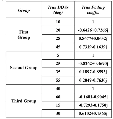
Table 4.1: True values of DOAs and fading coefficients for the first, second and third groups

Group True DOAs _(deg) True Fading _coeffs.

First Group 10 1 20 -0.6426+0.7266j 28 0.8677+0.0632j 45 0.7319-0.1639j Second Group 5 1 25 -0.8262+0.4690j 35 0.1897-0.8593j 55 0.2049-0.7630j Third Group 40 1 60 -0.1681-0.9045j 15 -0.7293-0.1750j 30 0.6102+0.1565j

The true arrival angles and mean values of estimated angles as the average of 50 trials for root-MUSIC, MFBLP and ESPRIT DOA methods are given in Table 4.2 while Fig. 4.1 and 4.2 give the spectrums for Min-norm and MUSIC respectively. The mean value of the DOAs is given as:

 







Table 4.2: True arrival angles and mean of estimated DOA angles for Ns=2000, M=12, T=50 trials and SNR=10dB case

True Angles (degrees)

Mean of Estimated Angles with High Resolution Methods (degrees)

Root-MUSIC MFBLP ESPRIT

10 10.0843 10.0632 9.9997 20 20.5100 20.1556 20.1997

True Angles (degrees)

Mean of Estimated Angles with High Resolution Methods (degrees)

Root-MUSIC MFBLP ESPRIT 28 27.5114 27.9078 27.8078 45 45.0938 45.0698 44.9773 5 4.9969 5.0030 5.0022 25 24.8704 24.8885 24.9980 35 34.8160 34.8742 35.0617 55 55.0399 55.0271 54.9718 40 39.8429 39.9967 39.9286 60 59.9566 59.9985 59.8564 15 15.0480 15.0256 14.9378 30 29.9608 30.0429 29.9803 (a) -100 -80 -60 -40 -20 0 20 40 60 80 100 -10 -5 0 5 10 15 20 25

Angle of Arrival (degrees)

M in -n o rm S p a ti a l S p e c tr u m ( d B )

First Coherent Signals group

X: 20.5 Y: 20.83 X: 10 Y: 21.62 X: 27.4 Y: 21.96 X: 45 Y: 22.19

(b)

(c)

Figure4.1: The estimation of Min-norm spectrum for (a) the first signal group (b) the second signal group (c) the third signal group, for 50 Monte-Carlo trials. The high peaks indicate the estimated DOAs of the signals.

-100 -80 -60 -40 -20 0 20 40 60 80 100 -10 -5 0 5 10 15 20 25 30

Angle of Arrival (degrees)

M in -n o rm S p a ti a l S p e c tr u m ( d B )

Second Coherent Signals group

X: 24.8 Y: 26.46 X: 5 Y: 23.24 X: 34.8 Y: 29.75 X: 55.1 Y: 22.05 -100 -80 -60 -40 -20 0 20 40 60 80 100 -10 -5 0 5 10 15 20 25 30

Angle of Arrival (degrees)

M in -n o rm S p a ti a l S p e c tr u m ( d B )

Third Coherent Signals group

X: 14.9 Y: 21.04 X: 29.3 Y: 25.94 X: 40.4 Y: 22.87 X: 60 Y: 23.32

(a) (b) -1000 -80 -60 -40 -20 0 20 40 60 80 100 10 20 30 40 50 60 X: 10.2 Y: 54.44

First Coherent Signals group

Angle of Arrival (degrees)

M U S IC S p a ti a l S p e c tr u m ( d B ) X: 20.6 Y: 47.57 X: 27.6 Y: 47.73 X: 45 Y: 53.26 -1000 -80 -60 -40 -20 0 20 40 60 80 100 10 20 30 40 50 60 70

Second Coherent Signals group

Angle of Arrival (degrees)

M U S IC S p a ti a l S p e c tr u m ( d B ) X: 5 Y: 62.86 X: 25 Y: 61.87 X: 35.1 Y: 60.36 X: 55 Y: 60.88