ERROR RESILIENT STEREOSCOPIC VIDEO
STREAMING USING MODEL-BASED FOUNTAIN
CODES
a dissertation
submitted to the department of electrical and
electronics engineering
and the institute of engineering and science
of b
˙Ilkent university
in partial fulfillment of the requirements
for the degree of
doctor of philosophy
By
A. Serdar Tan
January 2009
I certify that I have read this thesis and that in my opinion it is fully adequate, in scope and in quality, as a dissertation for the degree of doctor of philosophy.
Prof. Dr. Erdal Arıkan (Supervisor)
I certify that I have read this thesis and that in my opinion it is fully adequate, in scope and in quality, as a dissertation for the degree of doctor of philosophy.
Prof. Dr. Levent Onural
I certify that I have read this thesis and that in my opinion it is fully adequate, in scope and in quality, as a dissertation for the degree of doctor of philosophy.
I certify that I have read this thesis and that in my opinion it is fully adequate, in scope and in quality, as a dissertation for the degree of doctor of philosophy.
Assoc. Prof. Dr. U˘gur G¨ud¨ukbay
I certify that I have read this thesis and that in my opinion it is fully adequate, in scope and in quality, as a dissertation for the degree of doctor of philosophy.
Asst. Prof. Dr. Defne Akta¸s
Approved for the Institute of Engineering and Science:
ABSTRACT
ERROR RESILIENT STEREOSCOPIC VIDEO
STREAMING USING MODEL-BASED FOUNTAIN
CODES
A. Serdar Tan
Ph.D. in Electrical and Electronics Engineering
Supervisor: Prof. Dr. Erdal Arıkan
January 2009
Error resilient digital video streaming has been a challenging problem since the introduction and deployment of early packet switched networks. One of the most recent advances in video coding is observed on multi-view video cod-ing which suggests methods for the compression of correlated multiple image sequences. The existing multi-view compression techniques increase the loss sen-sitivity and necessitate the use of efficient loss recovery schemes. Forward Error Correction (FEC) is an efficient, powerful and practical tool for the recovery of lost data. A novel class of FEC codes is Fountain codes which are suitable to be used with recent video codecs, such as H.264/AVC, and LT and Raptor codes are practical examples of this class. Although there are many studies on monoscopic video, transmission of multi-view video through lossy channels with FEC have not been explored yet. Aiming at this deficiency, an H.264-based multi-view video codec and a model-based Fountain code are combined to generate an effi-cient error resilient stereoscopic streaming system. Three layers of stereoscopic video with unequal importance are defined in order to exploit the benefits of Un-equal Error Protection (UEP) with FEC. Simply, these layers correspond to intra
frames of left view, predicted frames of left view and predicted frames of right view. The Rate-Distortion (RD) characteristics of these dependent layers are de-fined by extending the RD characteristics of monoscopic video. The parameters of the models are obtained with curve fitting using the RD samples of the video, and satisfactory results are achieved where the average difference between the analytical models and RD samples is between 1.00% and 9.19%. An heuristic analytical model of the performance of Raptor codes is used to obtain the resid-ual number of lost packets for given channel bit rate, loss rate, and protection rate. This residual number is multiplied with the estimated average distortion of the loss of a single Network Abstraction Layer (NAL) unit to obtain the total transmission distortion. All these models are combined to minimize the end-to-end distortion and obtain optimal encoder bit rates and UEP rates. When the proposed system is used, the simulation results demonstrate up to 2dB increase in quality compared to equal error protection and only left view error protec-tion. Furthermore, Fountain codes are analyzed in the finite length region, and iterative performance models are derived without any assumptions or asymp-totical approximations. The performance model of the belief-propagation (BP) decoder approximates either the behavior of a single simulation results or their average depending on the parameters of the LT code. The performance model of the maximum likelihood decoder approximates the average of simulation results more accurately compared to the model of the BP decoder. Raptor codes are modeled heuristically based on the exponential decay observed on the simulation results, and the model parameters are obtained by line of best fit. The analytical models of systematic and non-systematic Raptor codes accurately approximate the experimental average performance.
Keywords: Fountain Codes, Forward Error Correction, Video Streaming, Stereo-scopic Video.
¨
OZET
MODEL TABANLI FOUNTAIN KODLARI KULLANARAK
HATAYA DAYANIKLI STEREO V˙IDEO AKITIMI
A. Serdar Tan
Elektrik ve Elektronik M¨uhendisli¯gi B¨ol¨um¨u Doktora
Tez Y¨oneticisi: Prof. Dr. Erdal Arıkan
Ocak 2009
Hataya dayanıklı sayısal video akıtımı, paket anahtarlamalı a˘gların ortaya ¸cıkmasından ve yayılmasından bu yana ilgi ¸cekici ve zor bir problem olmu¸stur. Video kodlama alanındaki en yeni geli¸smelerden biri ilinliti ¸coklu imge dizilerinde sıkı¸stırma i¸cin metodlar ¨oneren ¸cok-g¨or¨u¸sl¨u kodlayıcı-¸c¨oz¨uc¨ulerde g¨or¨ulmektedir. Mevcut ¸cok-g¨or¨u¸sl¨u sıkı¸stırma teknikleri yitimlere olan duyarlılı˘gı arttırmakta ve yitim kurtarma y¨ontemlerinin kullanımını gerektirmektedir. G¨onderme Y¨on¨unde Hata D¨uzeltimi (GYHD) yitik verilerin kurtarılması i¸cin verimli, kuvvetli ve uygulanabilir bir ara¸ctır. Fountain kodları GYHD kodlarının yeni bir sınıfıdır ve LT ve Raptor kodları bu sınıfın uygulanabilir ¨ornekleridir. Bu kodlar H.264/AVC gibi en yeni video kodlayıcı-¸c¨oz¨uc¨uler ile uyumlu ¸calı¸sabilmektedir. Tek g¨or¨u¸sl¨u video ile ilgili bir ¸cok ¸calı¸sma olmasına ra˘gmen, ¸cok-g¨or¨u¸sl¨u videonun yitimli kanallarda GYHD ile iletimi yeteri kadar incelenmemi¸stir. Bu eksikli˘gi hedef alarak, verimli ve hataya dayanıklı bir stereo video akıtım sistemi olu¸sturmak i¸cin H.264 temelli ¸cok-g¨or¨u¸sl¨u bir video kodlayıcı-¸c¨oz¨uc¨u ve model temelli bir Fountain kodu bir arada kullanılmı¸stır. GYHD ile birlikte e¸sit olmayan hata koruması (EOHK) kullanmanın faydalarından yararlanmak i¸cin stereo video-nun farklı ¨onemlere sahip ¨u¸c katmanı tanımlanmı¸stır. Temel olarak, bu ¨u¸c
katman sol g¨or¨u¸s¨un ¸cer¸ceve i¸ci kodlanmı¸s ¸cerceveleri, sol g¨or¨u¸s¨un ¨ong¨or¨ulm¨u¸s ¸cer¸ceveleri ve sa˘g g¨or¨u¸s¨un ¨ong¨or¨ulm¨u¸s ¸cer¸cevelerinden olu¸sur. Tek g¨or¨u¸sl¨u videonun Hız-Bozulum (HB) karakteristi˘gi geni¸sletilerek ba˘gımlı katmanların HB karakteristi˘gi tanımlanmı¸stır. Videonun HB ¨orneklerini kullanarak e˘gri oturtma tekni˘gi ile model parametreleri elde edilmi¸stir, ve HB ¨ornekleri ile analitik model arasındaki ortalama farkın %1.00 ve %9.19 arasında oldu˘gu tatminkar sonu¸clar elde edilmi¸stir. Kanal bit hızı, kayıp oranı ve koruma oranı verildi˘ginde kalan kayıp paket sayısını elde etmek i¸cin Raptor kodlarının bulu¸ssal bir analitik modeli kullanılmı¸stır. Bu kalan sayı, tek bir A˘g Soyutlama Katmanı (ASK) biriminin yitiminden kaynaklanan kestirilmi¸s ortalama bozulum ile ¸carpılarak toplam iletim bozulumu elde edilmi¸stir. B¨ut¨un bu modeller, u¸ctan-uca bozulumu enk¨u¸c¨ultmek ve en iyi kodlayıcı bit hızlarını ve EOHK oranlarını elde etmek i¸cin birle¸stirilmi¸stir. ¨Onerilen sistem kullanıldı˘gında, e¸sit hata koruması ve sadece sol g¨or¨u¸s koruması y¨ontemleri ile kar¸sıla¸stırıldı˘gında, benzetim sonu¸cları 2dB’ye varan kalite artı¸sı g¨ostermi¸stir. Bundan ba¸ska, Fountain kodları sonlu uzunluk b¨olgesinde analiz edilmi¸s ve varsayımlar ya da asimtotik yakla¸sıklamalar olmadan d¨ong¨ul¨u ba¸sarım modelleri t¨uretilmi¸stir. ˙Inan¸c-Yayılım (˙IY) kod¸c¨oz¨uc¨us¨un¨un ba¸sarım modeli LT kodunun parametrelerine ba˘glı olarak ya tek bir benzetim sonucunu ya da bu sonu¸cların ortalamasını yakla¸sıklamı¸stır. En b¨uy¨uk olabilirlik kod¸c¨oz¨uc¨us¨un¨un ba¸sarım modeli, ˙IY kod¸c¨oz¨uc¨us¨un¨un modeli ile kıyaslandı˘gında, benzetim sonu¸clarının ortalamasını daha iyi yakla¸sıklamı¸stır. Raptor kodları, benzetim sonu¸clarında g¨or¨ulen ¨ustel azalmaya dayanarak, bulu¸ssal olarak model-lenmi¸s ve model parametreleri en iyi oturan do˘gru ile elde edilmi¸stir. Sistematik ve sistematik olmayan Raptor kodlarının anatilik modelleri deneysel ortalama ba¸sarımı do˘gru bir ¸sekilde yakla¸sıklamı¸stır.
Anahtar Kelimeler: Fountain Kodları, G¨onderme Y¨on¨unde Hata D¨uzeltimi, Kesintisiz Video ˙Iletimi, Stereo Video.
ACKNOWLEDGMENTS
I gratefully thank to my supervisor Prof. Dr. Erdal Arıkan for his guidance, support and keen concern throughout the development of this thesis. I would like to express my gratitude to the members of the thesis monitoring committee Prof. Dr. Levent Onural and Prof. Dr. G¨ozde Bozda˘gı Akar for their valuable comments and guidance. I would also like to thank the committee members Assoc. Prof. Dr. U˘gur G¨ud¨ukbay and Asst. Prof. Dr. Defne Akta¸s for accepting to read the manuscript and commenting on the thesis.
I would also like to thank the members of the Multimedia Research Group of Prof. Dr. G¨ozde Bozda˘gı Akar in METU. I specially thank to Anıl Aksay for his collaboration.
Special thanks to Namık S¸engezer, Ay¸ca ¨Oz¸celikkale, Mehmet K¨oseo˘glu, Kıva¸c K¨ose, G¨okhan Bora Esmer, Yi˘gitcan Eryaman, Av¸sar Polat Ay, Onur Ta¸s¸cı, Kaan Do˘gan, G¨uray G¨urel, Sıla Kurug¨ol and Onur Afacan for making the past 5 years of the office life enjoyable with their endless support and friendship.
It is a great pleasure to express my gratitude to my family Kezban, Mustafa, Ay¸se and Mehmet Tan. Without their support, this work would not be possible. Finally, I sincerely thank to my love Selin for making me love the life and making the thesis process bearable.
This thesis work is supported by the EC under contract FP6-511568 3DTV and by the graduate scholarship program of T ¨UB˙ITAK (Scientific and Technical Research Council of Turkey).
Contents
1 Introduction 1
1.1 Problem Statement . . . 1
1.2 Background . . . 2
1.2.1 Error Correction . . . 2
1.2.2 Video Coding and Streaming . . . 6
1.3 Contributions . . . 7
1.4 Outline . . . 8
2 Related Work and Definitions 10 2.1 Basics of Fountain Coding . . . 10
2.2 Random X-OR codes . . . 13
2.3 Tornado Codes . . . 16
2.4 LT Codes . . . 16
2.5 Raptor Codes . . . 21
2.5.1 Encoder . . . 21
2.5.2 Decoder . . . 22
2.6 Video Coding and Streaming . . . 22
2.6.1 History of Video Coding Standards . . . 22
2.6.2 Video Compression Principles . . . 25
2.6.3 Video Streaming Principles . . . 27
2.7 Multi-view Video Coding and Streaming . . . 28
2.8 Error Resilient Video Streaming with Fountain Codes . . . 30
2.9 Improving the State-of-the-Art Techniques . . . 31
3 Error Correction in Stereoscopic Video Streaming 32 3.1 Motivation . . . 32
3.2 Basics of Error Resiliency Techniques for Video Streaming . . . . 33
3.2.1 Error Concealment . . . 34
3.2.2 Flexible Macroblock Ordering . . . 35
3.2.3 Forward Error Correction . . . 36
3.3 Overview of the Video Streaming System . . . 38
3.4 Modeling the Rate-Distortion Curve of Stereoscopic Video . . . . 39
3.4.2 RD Curve Models for the Layers of Stereoscopic Video . . 40
3.4.3 Results . . . 42
3.4.4 Optimization on Encoder RD curve . . . 48
3.5 Modeling the Performance of Raptor Codes . . . 49
3.6 Modeling the Error Propagation in Video . . . 50
3.6.1 Lossy Transmission . . . 50
3.6.2 Reconstruction of Input Symbols in Raptor Decoder . . . . 51
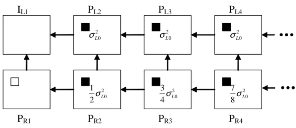
3.6.3 Propagation of Lost NAL units in Stereoscopic Video De-coder . . . 51
3.6.4 Calculation of Residual Loss Distortion . . . 57
3.7 Distortion Minimization and Results . . . 57
3.7.1 Results on the Minimization of End-to-End Distortion . . 59
3.7.2 Simulation Results . . . 59
4 Analysis and Modeling of Fountain Codes 67 4.1 Motivation . . . 67
4.2 Design of Degree Distributions . . . 68
4.2.1 Degree Distribution of LT Codes . . . 68
4.2.2 Degree Distribution of Raptor Codes . . . 74
4.5 General Method for the Analysis of Fountain Codes . . . 80
4.5.1 The Analysis of LT BP Decoder . . . 80
4.5.2 Modeling the Performance Curve of LT BP Decoder . . . . 83
4.5.3 Modeling the Performance Curve of LT ML Decoder . . . 89
4.5.4 Modeling the Performance Curve of Raptor Decoder . . . . 91
5 Conclusions 97
List of Figures
1.1 The protocol stacks for video streaming . . . 3
2.1 Overview of Fountain coding: The decoders (bins) try to collect sufficient number of output symbols (water drops) . . . 11
2.2 Bipartite graph for LT coding . . . 17
2.3 A step in the LT BP decoder . . . 19
2.4 The representation of the Raptor encoder . . . 21
2.5 An example reference structure in video coding . . . 25
2.6 Block-based motion estimation in inter-frames . . . 27
2.7 An example reference structure in multi-view video coding . . . . 29
3.1 The representation of two basic error concealment techniques, (a) spatial, (b) temporal . . . 34
3.2 The results on the effect of error concealment on video quality . . 35
3.3 The results on the effect of FMO on video quality . . . 36
3.5 Overview of the stereoscopic streaming system . . . 38
3.6 The layers of stereoscopic video and reference structure . . . 40
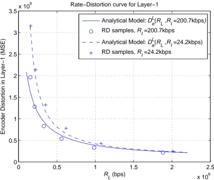
3.7 The RD curve for Layer 0 of the ‘Rena’ video . . . 45
3.8 The RD curve for Layer 0 of the ‘Soccer’ video . . . 45
3.9 The RD curve for Layer 1 of the ‘Rena’ video . . . 46
3.10 The RD curve for Layer 1 of the ‘Soccer’ video . . . 46
3.11 The RD curve for Layer 2 of the ‘Rena’ video . . . 47
3.12 The RD curve for Layer 2 of the ‘Soccer’ video . . . 47
3.13 The RD curve for 3 layers . . . 49
3.14 The propagation of a MB loss from I-frame . . . 53
3.15 The propagation of a MB loss from L-frame . . . 54
3.16 The propagation of a MB loss from R-frame . . . 56
3.17 The results for pe = 0.03 for the ‘Rena’ video . . . 63
3.18 The results for pe = 0.05 for the ‘Rena’ video . . . 63
3.19 The results for pe = 0.10 for the ‘Rena’ video . . . 64
3.20 The results for pe = 0.20 for the ‘Rena’ video . . . 64
3.21 The results for pe = 0.03 for the ‘Soccer’ video . . . 65
3.22 The results for pe = 0.05 for the ‘Soccer’ video . . . 65
3.23 The results for pe = 0.10 for the ‘Soccer’ video . . . 66
4.1 LT process at step t . . . 71
4.2 The overhead of LT codes . . . 76
4.3 The performance curve of LT codes with Robust Soliton distri-bution, k = 500, c = 0.7 and δ = 0.001, (a) LT BP decoder, (b) LT ML decoder . . . 77
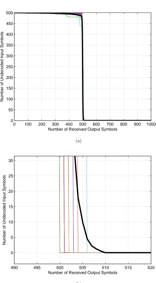
4.4 The performance curve of Raptor Codes with the Raptor distri-bution in Table 4.2, k = 500, (a) Whole Performance, (b) Perfor-mance zoomed around 500 received output symbols . . . 79
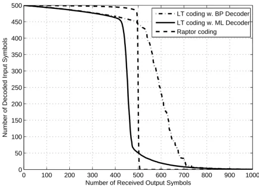
4.5 The comparison of the performance of LT codes with ML and BP decoder and Raptor codes . . . 80
4.6 The comparison of the analytical and simulation results on LT BP decoder . . . 84
4.7 Modeling the performance of LT BP decoder. Black bold solid line: model, black bold dashed line: the average of simulations. (a) c = 0.7, δ = 0.001, (b) c = 0.02, δ = 0.001 . . . 88
4.8 The representation of two vectors corresponding to two output symbols with degrees j and l . . . 89
4.9 The comparison of the analytical model and simulation results on the LT ML decoder . . . 91
4.10 The results on modeling the performance of non-systematic Rap-tor codes (a) whole performance for k = 200 (b) normalized log-scale plot for r ≥ k for k = 100, k = 200 and k = 500 . . . 93
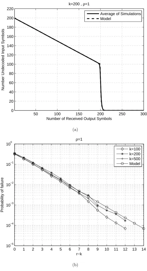
4.11 The results on modeling the performance of systematic Raptor codes for ρ = 1.0 (a) whole performance for k = 200 (b) normal-ized log-scale plot for r ≥ k for k = 100, k = 200 and k = 500 . . 95
4.12 The results on modeling the performance of systematic Raptor codes for ρ = 0.5 (a) whole performance for k = 200 (b) normal-ized log-scale plot for r ≥ k for k = 100, k = 200 and k = 500 . . 96
List of Tables
3.1 Encoder RD curve parameters for the ‘Rena’ and ‘Soccer’ videos . 43
3.2 The video encoder bit rates and Raptor encoder protection rates for the ‘Rena’ video . . . 60
3.3 The video encoder bit rates and Raptor encoder protection rates for the ‘Soccer’ video . . . 61
4.1 The Ideal and Robust Soliton distributions for k = 500 (δ = 0.01,
c = 0.1 for Robust Soliton) . . . 73
Chapter 1
Introduction
Video streaming through lossy channels has received considerable attention for the past 20 years. The worldwide increases in the number of Internet access, dedicated bandwidth and video sharing websites have triggered the research.
1.1
Problem Statement
Increasingly more and more data have to be distributed over lossy transmis-sion channels with limited bandwidth. Stereoscopic video is emerging as a new source of data for the next generation communication systems. Owing to its high bandwidth and loss sensitivity, optimal transmission strategies for stereoscopic video should be derived to obtain efficiency. Furthermore, optimal transmission through lossy channels necessitates the use of the most advanced error correction schemes and their corresponding analysis.
There are some constraints on such a system in order to be deployed over existing infrastructure. First of all, it has to be simple and piecewise analyzable. The system has to be efficient and optimal in a sense that it compensates the simple design. Flexibility and scalability, which are required for the ease of bit
rate adaptability, are also important constraints. Finally, the system has to be robust against transmission errors, the main reason of the distortion in video quality. Thus, the chosen error correction scheme has to be fully analyzed and understood.
In this thesis, we consider optimal transmission strategies for an end-to-end stereoscopic streaming system that uses an H.264-based multi-view video codec. We use a Fountain code for recovery from packet losses, and investigate their performance in detail.
1.2
Background
The data losses during transmission in Internet are observed due to several rea-sons. In order to understand the sources of error, we should look at the protocol stacks. In Figure 1.1, the protocol stacks specific to a recent video codec, H.264, are presented. The transmission errors occur only in the IP and physical layers. In the physical layer, bit errors occur due to the noise in the transmission. In the IP layer, packet losses occur due to congestion in the routers. Caused by either physical or IP layer, the error is observed as packet loss in the upper layers. In order to protect from the packet losses in video streaming, application layer For-ward Error Correction (FEC) can be used. In such a scenario, the place of the FEC is demonstrated in Figure 1.1. In the following sections, we briefly define error correction and video streaming.
1.2.1
Error Correction
After Shannon defined the fundamentals of channel capacity in the landmark pa-per [1] in 1948, many researchers around the world studied different techniques
Physical Data Link Internet Protocol (IP)
Transport Control Protocol (TCP) User Datagram Protocol (UDP)
Hypertext Transfer Protocol
(HTTP)
Real-time Transport Protocol (RTP) Real-Time
Streaming Protocol (RTSP)
Forward Error
Correction (FEC) MPEG-2 TS
Network Abstraction Layer (NAL) Video Coding Layer (VCL)
Figure 1.1: The protocol stacks for video streaming
Among these, FEC scheme came out to be one of the best way of approaching channel capacity in a feedback-free transmission system. In an FEC scheme, the encoder introduces redundant bits to the original message. Then, in case of any losses, the decoder tries to recover the original message with the help of these redundant bits. Some of the primary examples of FEC codes are Hamming codes [2], BCH codes [3], Reed-solomon (RS) codes [4] etc.. Among these pri-mary examples RS coding is the most notable due to its widespread deployment in current storage media such as CDs, DVDs and HDDs. The encoding and decoding of the primary examples are problematic for large message lengths due to their high complexities. One of the recently used, but not recently invented examples of FEC codes is low-density parity-check (LDPC) codes. Invented in 1960 by Gallager [5], LDPC codes were impractical to implement, because they are capacity approaching for very large message lengths. Three decades later, LDPC codes were rediscovered and took place in many standards such as Digital Video Broadcasting - Satellite - Second Generation (DVB-S2) [6] in 2003. In this standard, message length varies from 16200 to 64800 bits. Using the belief prop-agation decoding [7] with large message lengths, LDPC coding is nearly capacity
achieving as shown in [8]. Operating on the sparse (low density) parity check matrix, the belief propagation decoder can achieve a computational complexity linear with the message length. In the early 90s a novel FEC scheme, Turbo cod-ing [9] which combined two or more convolutional codes and a block interleaver that has led to another capacity approaching channel code, was proposed.
The general application area of LDPC and Turbo codes are on noisy channels such as Additive White Gaussian Noise Channel (AWGNC), Binary Symmetric Channel (BSC) or Binary Erasure Channel (BEC). These codes are implemented on the physical layer of transmission systems. However, the most widely deployed networks are wired packet switched networks, such as Internet, and the source of error in these networks is packet loss which is generally caused by congestion or other network problems, and not usually by physical layer errors. Thus applying channel coding in physical layer is not a proper way of protection in these net-works. The underlying channel in packet switched networks is denoted as packet erasure channel (PEC). In the PEC a packet is either received completely intact and error free or it is lost. Thus, a lost packet with all its bits is the erasure.
The most widely deployed error detection/correction technique for PEC is the Automatic Repeat Request (ARQ) scheme that the Transport Control Protocol (TCP) utilizes. In the ARQ scheme the receiver detects missing packets and automatically requests their retransmission from the source. The transmission of the packets is ordered, so that when a packet is lost subsequent packets wait the retransmission of the lost packet. This scheme may cause feedback implosion in a broadcasting scenario, especially when the loss rate is high.
A novel technique that recently became popular for error protection in lossy packet networks is Fountain codes which is also called rateless codes. The Foun-tain coding idea is proposed in [10] and followed by practical realizations such as (Luby Transform) LT codes [11] and Raptor codes [12]. Raptor codes are
ex-Fountain codes remove the necessity of orderly transmission and retransmissions which prevents the feedback implosion that occurs when ARQ is used. They also produce as many parity packets as needed on-the-fly. This approach is different than the general idea of FEC codes where channel encoding is performed for a fixed channel rate and all encoded packets are generated prior to transmission. In the traditional FEC codes, if the number of losses exceeds a certain amount, then the code cannot be extended on-the-fly to have a lower rate to achieve higher loss protection.
LT codes achieve on-the-fly rate extension capability and low complexity in exchange of some performance. Their performance depends on two factors. First one is the degree distribution which is used for generating the output symbols from the input symbols, and it has direct effect on encoding and decoding com-plexities. Thus, the degree distribution is designed so that it minimizes the complexity. Second factor is the block length, namely the number of input sym-bols. The performance of Raptor codes are affected by another factor which is the pre-coding stage. Fountain codes are asymptotically optimal, hence they operate efficiently when the number of input symbols is very high. However, Rap-tor codes are an exception, because their performance is quite acceptable for low number of input symbols, as well. The analysis of the performance, depending on the degree distribution and block length, needs detailed study to obtain accurate results. In [13], an analysis of the performance of LT codes yielded an iterative analytical model of their performance with significant high complexity. In [12], rather than exact analysis and modeling, some bounds on the performance of LT codes and Raptor codes are presented. The analysis and modeling of fountain codes are beneficial for optimization in end-to-end transmission systems.
Although being recently proposed, fountain codes are protected by several patents and appear in several standards. Raptor codes appear in the standards
Digital Video Broadcast for Hand-held (DVB-H) [14] and 3rd Generation
Part-nership Project (3GPP) [15] in multimedia broadcast. In both of the standards Raptor coding is applied as an application layer FEC to recover the lost packets and the details on the Raptor codec is described in the IETF draft in [16].
1.2.2
Video Coding and Streaming
First practically applicable video coding standards appeared in the early 90s such as H.261 [17] in 1990 and MPEG-1 [18] in 1991. Since then, the compression effi-ciency of the codecs have increased and many novel tools have been introduced. The main idea in video compression in the recent video codecs is similar to the early ones. Currently, all of the available video codecs use the temporal depen-dency between subsequent frames to achieve compression. Fundamentally, the frames are divided into two groups: Intra-frames and inter-frames. The intra-frames are compressed by standard still image compression techniques, similar to JPEG [19], thus they are self-decodable. Generally, the location of the intra-frames determines the beginning of group of pictures (GOP). The remaining frames that reside between intra-frames are called inter-frames. Inter-frames are compressed by using one or more previous or subsequent frames, eventually us-ing intra-frames, and most of the gain in video compression is achieved by this feature.
Video streams often have some scalability or unequal loss sensitivity. Basi-cally, the loss of the packets of intra-frames reduce the quality of video more than the loss of the packets of inter-frames. Because inter-frames are useless without the intra-frames. Thus, intra-frames need more protection against losses. Sim-ilarly, some parts of the images in a video may have more dominant motion characteristics. This leads to Flexible Macroblock Ordering (FMO) [20], [21]
elements of video, such as dc and ac coefficients, motion vectors, headers etc., based on their sensitivity to errors. Unequal loss sensitivity exists in scalable video codecs where the bitstream is composed of base layer and enhancement layers. Scalable video coding uses techniques such as spatial, temporal or SNR scalability. In [24], the Scalable Video Coding (SVC) extension of H.264/AVC is explained in a broader sense. In the cases where the video data parts have unequal loss sensitivity, utilization of unequal error protection (UEP) offers sig-nificant increase in video quality.
In order to further improve the visual experience, 3-dimensional video coding techniques are also proposed. Multi-view video coding is an extension of stan-dard single-view (monoscopic) video coding techniques to more than one views (cameras) [25], [26]. Multi-view video is formed by the simultaneous capture of a scene by more than one cameras which are separated with an acceptable dis-tance. Eventually, capturing more than one video sequence increases the amount of source data. Existing multi-view coding techniques tries to reduce the size by the compression techniques that exploit the dependency between these views. For this purpose, a new technique, inter-spatial frame coding is introduced and used, besides intra and inter-frame coding. The sophisticated structure of multi-view compression and increased dependencies between frames deduces even more data groups with different loss sensitivities.
1.3
Contributions
In this thesis, we specifically focus on stereoscopic video streaming. Numer-ous components have to be combined to work harmoniNumer-ously in order to realize streaming in lossy channels. Consequently, it is very difficult, if not impossible, to obtain an optimal end-to-end streaming system. In this sense, since there exist numerous parameters, stereoscopic video streaming in lossy transmission
channels with FEC becomes a quite difficult joint source-channel coding prob-lem. Thus, one needs to simplify the problem and handle it by dividing into smaller pieces in exchange of moving away from optimality a little bit. In this thesis, we specify the most important contributions as; basic partitioning of the video according to unequal importance, obtaining rate-distortion properties of these partitions, analysis of the utilized FEC scheme for UEP, and end-to-end distortion minimization. We provide separate analysis for each part and obtain mathematical models that we use for distortion minimization. The proposed an-alytical models for RD curve of the layers and performance of Raptor codes are quite accurate. After estimating the average distortion of a single lost packet, we define a model for end-to-end distortion, namely the sum of encoder and trans-mission distortions, and minimize it to obtain the optimal encoder and protection bit rates.
Apart from the stereoscopic video streaming, we also focus on the analysis of Fountain codes in detail. We aimed at the deficiency of analytical modeling in the literature for fountain codes that would be beneficial in the optimization of video streaming systems for lossy transmission. We give special attention to LT codes with Belief Propagation (BP) and Maximum Likelihood (ML) decoder and systematic and non-systematic Raptor codes. We contribute in two ways, first by providing a detailed analysis of these codes, and second, by proposing analytical models for their performances.
1.4
Outline
The organization of the thesis follows. In Chapter 2, we present the basics of Fountain codes and video streaming with their historical overviews. We describe the operation of Fountain codes with intuitive examples and explain video coding
streaming. Then, we analyze the components of stereoscopic video streaming and propose an error-resilient system with Fountain codes. In Chapter 4, initially, we describe the operation of Fountain codes in detail and present performance results with simulations. Then, we analyze them and propose analytical performance models. In Chapter 5, we conclude and state possible future work.
Chapter 2
Related Work and Definitions
2.1
Basics of Fountain Coding
The idea of Fountain coding is different from the original FEC idea where chan-nel encoding is performed for a fixed chanchan-nel rate and all encoded packets are generated prior to transmission. The Fountain encoder is an imaginary fountain of limitless supply of water drops (output symbols). Any person who wants to reconstruct all of the input symbols has to wait to fill their bucket with slightly more water drops than the number of input symbols. Thus, the main idea be-hind Fountain coding is to produce as many output symbols as needed on-the-fly. This property gave another name to fountain codes, rateless codes.
The principle of Fountain codes is illustrated in Figure 2.1. The encoder generates potentially limitless output symbols (water drops) from the input data. The decoder (bins) try to collect enough number of output symbols to complete decoding and reconstruct the input symbols. During the transmission (collecting water drops), output symbols may get lost due to the channel conditions. In such a case, decoders do not send any retransmission request messages back to
Figure 2.1: Overview of Fountain coding: The decoders (bins) try to collect sufficient number of output symbols (water drops)
the encoder. They just wait to receive enough number of output symbols to complete the decoding.
Digital Fountain approach is first described in 1998 as a novel technique for reliable distribution of bulk data [10]. In the same year, a company named Digital Fountain Inc. is founded by Charlie Oppenheimer and Dr. Michael Luby in CA, U.S. with the aim of commercializing and standardizing the fountain coding approach. In 1999, first patent on fountain coding appeared [27], and it has been revised several times under same title [28], [29], [30], [31]. In 2002, Luby Transform (LT) codes, named after Michael Luby, are published in [11] that described the coding scheme in the patents. The coding scheme attracted significant interest and various papers on LT codes have been published since then.
Raptor coding is proposed as a multi-stage extension of LT coding. They are invented in 2000 and patented [32]. Publication of Raptor codes appeared first in a technical report in 2003 [33] and then in 2006 [12]. They are still one of the most advanced fountain coding scheme, and similar to LT coding, attracted a wide interest.
As mentioned in [11], the original idea and purpose of LT codes is the dis-tribution of bulk data to many users. Most common application area is the distribution of a service pack of an operating system to many computers in the world. In such a scenario the number of users will be huge and each user will experience different channel characteristics. If standard techniques are used such as TCP, the server and client has to communicate for each lost packet. Fountain codes are a candidate for this situation for reliable feedback-free transmission where users just wait to receive enough packets.
LT codes are considered suitable also for data storage in hard drives. Orig-inally, the data in hard drives are stored in successive segments, and when the reading head misses one track it has to retrace to read again which causes signif-icant delays. On the other hand, if fountain approach is used, the head does not have to retrace; it just skips and reads enough number of next segments. Thus, the hard drive can operate faster.
The encoding and decoding of LT codes are also defined in [11]. However, the proposed decoding algorithm is asymptotically optimal, which necessitates large block lengths. Thus, the problematic operation of LT codes on short and medium block lengths lead the introduction of ML decoder. Eventually, ML decoder performs better and its complexity is higher compared to original decoder, but for short block lengths its complexity might be acceptable.
many applications, because Raptor codes have reasonably better performance than their prior LT codes. The main target became distribution of multimedia data, such as video. Because video has sufficiently large block size and Raptor codes have low latency in encoding and decoding, which allows real-time error protection.
In order to be more suitable for multimedia distribution, the structure of fountain codes are also modified. Their original structure was non-systematic, namely each generated symbol is obtained by transforming the input symbols to new symbols. This property causes an all or nothing code where all of the symbols are either undecoded or decoded according to the loss rate of the transmission channel. For time limited applications, where destination may not wait for more output symbols, such as video streaming, this may become devastating. Treating the fountain codes as a fixed rate FEC code, systematic fountain coding is also proposed. By this way, partial recovery of data is still possible in case of excessive packet losses. This process requires limited time which may seem controversial to fountain coding approach; however, fast (low complexity) encoding and decoding of fountain codes render them suitable for time limited applications, as well.
In the following sections, we describe the widely known Fountain codes; ran-dom X-OR, Tornado, LT and Raptor codes which have attracted significant interest in the recent years.
2.2
Random X-OR codes
Random X-OR coding is the simplest of Fountain codes where each output sym-bol is generated as a random X-OR sum of the input symsym-bols. Let Ii be the row
vector os size s that denotes the ith input symbol (1 ≤ i ≤ k), and O
j be the row
to represent the generation of random output symbols, let Aj = [aj,1, aj,2, ..., aj,k]
denote the generator vector of jth output symbol, where
aj,i = 0 w.p. 1/2 1 w.p. 1/2 for 1 ≤ j, 1 ≤ i ≤ k . (2.1) Furthermore, let I = I1 ... Ik , A = A1 A2 ... , O = O1 O2 ... . (2.2)
Then, the generation of jth output symbol and the whole output symbols are
given, respectively as Oj = k M i=1 aj,iIi = Aj · I , (2.3) O = A · I . (2.4)
In (2.4), infinitely many output symbols, 2kof them being distinct, are generated
from k input symbols with the semi-infinite generator matrix A. The decoder tries to collect as many of these output symbols to reconstruct the input symbols.
A = 0 1 1 1 0 1 1 1 0 0 0 1 1 1 1 ... ... ... → → → × → ... , (2.5)
where × denotes loss and → denotes success during transmission. Having re-ceived the first three symbols, the decoder cannot reconstruct the input symbols since the Aj’s of the received symbols do not add up to a matrix with rank
3. When the fifth symbol arrives, after the fourth equation which was erased, the received generator matrix becomes full rank, namely all input symbols are determined.
In the decoding process, k independent output symbols must arrive for suc-cessful recovery. Let p(j) denote the probability that an arriving symbol is de-pendent when j indede-pendent symbols arrived previously, which can be calculated as p(j) = (1 − 2−(k−j)). Then, the average waiting time to receive the next
in-dependent symbol can be calculated as Wj = 1/p(j) by geometric random series
analysis. The total time to receive k independent symbols can be calculated as
k−1 X j=0 Wj = k−1 X j=0 1 (1 − 2−(k−j)) (2.6) = ∼ (k + 2) .
Thus, on the average, arrival of k + 2 output symbols ensures successful decod-ing of the input symbols. However, due to the O(k3) complexity of standard
elimination algorithms for dense matrices, the complexity of the decoder is the main drawback of X-OR codes. Lower complexity and efficient decoding algo-rithms can be achieved by using degree distributions for the generated output
symbols, where the number of X-OR summed input symbols will be chosen from a distribution, so that k X i=1 aj,i= dj , (2.7)
where dj is the degree of the jth output symbol chosen from a degree distribution.
2.3
Tornado Codes
Tornado codes [10], [34] are proposed to be the first example of fountain codes. They can generate infinitely many encoded symbols from k input symbols. When
k(1 + ε) of these input symbols arrive to the decoder, all of the k input symbols
can be decoded. However, the code is designed for a fixed number of encoded symbols n. The encoder can generate at most n output symbols and cannot produce more symbols on-the-fly. Moreover, the required overhead, kε, is at least a constant fraction of the number of input symbols. Due to this property we do not consider Tornado codes as an ideal fountain code.
2.4
LT Codes
LT codes proposed in [11] have initiated a novel research area. Instead of op-erating on low density parity check matrices, LT codes operate on low density generator matrices. In [11], it is shown that for large message length k LT codes are capacity achieving.
Figure 2.2: Bipartite graph for LT coding
2.4.1
Encoder
The unit of encoding in LT codes is called a symbol which is a data packet of size
m bits for some fixed m ≥ 1. Let the number of input symbols be k, then the
input data size is (k · m) bits. The number of the output symbols that can be generated from these input symbols is virtually limitless, i.e. the code is rateless. In Figure 2.2, generation of the first two output symbols are demonstrated on the encoding graph, where A1 = [1, 1, 0, ..., 0] and A2 = [1, 0, 1, 0, ..., 1]. In Figure 2.2,
the number of edges connected to an output symbol is its degree d, for example O1 has degree-2. The edges emanating from an output symbol of degree d are
connected randomly to d input symbols. These input symbols are denoted as the neighbors of the output symbols to which they are connected.
The number of lines that connect the input symbols to output symbols defines the complexity of the encoding process. Let ¯d represent the average degree of an
output symbol and assume that ¯d = ln (k). Then, based on the fact that k (1 + ε)
output symbols are enough to reconstruct the input symbols, the complexity is
2.4.2
Decoder
There are two different LT decoding schemes: Belief Propagation (BP) decoder and Maximum Likelihood (ML) decoder. BP decoder is the original low com-plexity decoder proposed in [11], but it is optimal for large values of k. ML decoder is the optimal decoder with high complexity.
Belief Propagation (BP) Decoder
Belief propagation decoding of LT codes is an iterative process best explained by an example. Assume that the number of input symbols is four, and the generator matrix and the received output symbols are given as
A = 1 1 0 0 1 0 0 0 0 1 0 1 0 1 1 1 0 0 1 1 ... ... ... ... → → → × → ... O1 = I1⊕ I2 O2 = I1 O3 = I2⊕ I4 O5 = I3⊕ I4 . (2.8)
Having received O1, the decoder can not decode I1 or I2. However, with O2, a
degree-1 output symbol, the decoder recovers I1 and I2 by I1 = O2, I2 = O1⊕ O2.
All of the steps of decoding for this specific example are given below.
• O2 = I1 ⇒ I1 is determined, • O1⊕ I1 ⇒ I2 is determined, • O3⊕ I2 ⇒ I4 is determined, • O5⊕ I2⊕ I4 ⇒ I3 is determined.
Figure 2.3: A step in the LT BP decoder
Initially, there exists an output symbol with degree 1 in the above example. If, there were no output symbols with degree 1 then the LT BP decoding procedure could not decode the input symbols with these set of output symbols. In such a case, the decoder has to wait for more output symbols to succeed in decoding. The algorithm of the BP decoding is given in the following steps, which are associated with the decoding phases in Figure 2.3.
1. Find an output symbol Oj that is connected to only one input symbol Ii,
i.e. find an output symbol with degree 1. If there is no such symbol the decoding fails (Phase-(a)).
2. Set Ii = Oj (Phase-(a)).
3. X-OR sum all of the output symbols that are connected to ithinput symbols
with its value Ii (Phase-(b)).
4. Remove the edges of the input symbol Ii from the graph (Phase-(c)).
5. Go to step 1 until all Ii are determined.
Similar to the encoder, the decoding complexity of this algorithm is propor-tional to the number of edges. When the average degree of an output symbol is
¯
d, and assuming that ¯d = ln(k), the complexity is O (k ln(k)) which is the same
as LT encoder.
Maximum Likelihood (ML) Decoder
In the belief propagation decoder, single degree output symbols have to exist throughout the decoding process. Consider the set of received output symbols
A = 1 1 0 0 1 0 0 0 0 1 0 1 0 1 1 1 0 0 1 1 ... ... ... ... → × → → → ... O1 = I1⊕ I2 O3 = I2⊕ I4 O4 = I2⊕ I3⊕ I4 O5 = I3⊕ I4 (2.9)
with the same generator matrix as (2.8) but with different received output sym-bols. Since a degree one output symbol does not exist, when these set of symbols are received the LT-BP decoder cannot determine any of the input symbols.
The ML decoder solves the system of linear equations in modulo-2 domain to reconstruct the input symbols Ii as
1 1 0 0 0 1 0 1 0 1 1 1 0 0 1 1 I1 I2 I3 I4 = O1 O3 O4 O5 . (2.10)
The LT-ML decoder solves the set of linear equations by straightforward linear algebra techniques. The difference from the random X-OR coding is the low
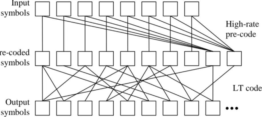
Output symbols Input symbols Pre-coded symbols High-rate pre-code LT code
Figure 2.4: The representation of the Raptor encoder
2.5
Raptor Codes
Raptor codes [12] are the most recent practical realization of Fountain codes and are an extension of LT codes. They have two consecutive channel encoders, where the pre-code is a high rate FEC code and the outer-code is an LT code. The pre-code generates the pre-coded symbols from the input symbols and the LT code generates output symbols from these pre-coded symbols.
2.5.1
Encoder
The complexity of the LT codes is O (k ln (k)) as explained in Section 2.4.2. The multiplicand ln (k) comes from the average degree ¯d. In order to make the
complexity linear with k, Raptor codes use a constant average degree in the LT coding phase. The constant average degree reduces the performance of the LT code, but the high-rate pre-code compensates this reduction.
An example to the construction of Raptor encoded symbols are given in Fig-ure 2.4. Initially, the high-rate pre-code generates k/ (1 − ˜e) pre-coded symbols which are not transmitted but used in an intermediate step to generate the transmitted output symbols. Then, LT coding with constant average degree is
applied to the pre-coded symbols. The details of the chosen pre-code and degree distribution are given in [12].
2.5.2
Decoder
The Raptor decoder begins to operate when slightly more than k output symbols arrive. After the LT decoder, using the balls and bins example in Section 4.2.1, the average number of source packets that remain unconnected in the graph can be calculated as e− ¯d = e−3 ∼= 0.05, when ¯d = 3. Thus, when k (1 + ε) output
symbols are received, 5% of the pre-coded symbols will remain undecoded. The pre-code is a perfect FEC code that can decode all input symbols when erasure rate is ˜e (the number of generated pre-codes was k/ (1 − ˜e)). When ˜e is chosen as 0.05 all of the input symbols can be decoded by the pre-code.
Instead of the simple pre-code we used in Figure 2.4, more sophisticated codes, such as LDPC codes [5], are used. Moreover, two stages of pre-codes are also defined such as the fully-specified Raptor FEC scheme defined in [16].
2.6
Video Coding and Streaming
2.6.1
History of Video Coding Standards
Video coding corresponds to the efficient representation, compression and trans-mission of image sequences. Studies on digital video processing have been virtu-ally initiated by the studies on digital image processing in 1960s. Current video coding techniques partially use the image compression techniques.
video codec aims at facilitating videoconferencing and videophone over the inte-grated digital services network (ISDN). The bit rate of the video signal, together with audio, can be varied from 64 kbps to 1.92 Mbps, for two image formats CIF (360x180) and QCIF (180x90). With the introduction of efficient compres-sion elements, such as inter-frame coding, motion compensation, discrete cosine transform (DCT), maximum delay of 150ms, ease of hardware implementation etc., H.261 standard is considered as the basis of latter video codecs.
In 1992, MPEG-1 was approved as an ISO video and audio coding standard whose details are given in [18]. The codec is proposed to progressively compress VHS quality video down to 1.5 Mbps for Video Compact Disc (VCD) storage. The codec does not standardize the compression mode, instead it specifies the coded bit stream and the decoder. In order to allow random access, periodic intra frames that are self decodable are introduced. Compared to H.261, the delay requirement of MPEG-1 is relaxed to 1 sec, because it does not aim bidirectional interactivity, instead unidirectional interactivity.
MPEG-2 [35] is a generic audio-video codec designed for two purposes; first, broadcast of TV signals at high bit rates, second, media storage on the Digital Versatile Discs (DVD). The video coding part, which is also known as H.262, is jointly developed by ISO and ITU-T teams, and the first standard appeared on 1994. Compared to MPEG-1, MPEG-2 supports a wider range of bit rates and resolutions; moreover it supports efficient tools for interlaced video. One of its most important specialities is the utilization of two different containers for the encoded video; first one is the transport stream that defines a communica-tion protocol for data multiplexing and loss recovery for unreliable transmission, whereas second one is the program stream that is designed for storage in reliable media, such as DVDs.
Later, in 1996, another video compression technique H.263 is proposed target-ing visual telephony, such as video conference similar to H.261, which is described
in [36]. The compressed data is aimed to be used on low bit rate networks such as ISDN and wireless networks. H.263 has a better performance than its prior H.261 with little additional complexity. An advanced version of H.263 is pro-posed in 1998 as H.263+, described in [37], with additional features, one of the most important being the introduction of scalability. Three modes of scalability are proposed; temporal, SNR and spatial scalability, which aim to improve the delivery of video information in error-prone and lossy packet networks.
The next codec, developed jointly by ITU-VCEG and MPEG teams, and completed in 2003, is the H.264 standard which is described in [24]. The codec has the largest area of application among all previous codecs, so that it ad-dresses all video telephony, storage, broadcast and streaming applications. The codec has the most advanced compression techniques and most flexible structure together with network friendly representation of the compressed data, so that compared to MPEG-2 the bit rate is reduced up to by half for high resolutions. H.264/AVC has two fundamental components; the Video Coding Layer (VCL) and the Network Abstraction Layer (NAL). The VCL is designed to efficiently compress the video, and the NAL is designed to format the compressed video and insert appropriate header information for transport layers or storage media. The scalable extension of the codec, which is described in [38], is completed in 2007. Currently, H.264/AVC is considered to be the state-of-the-art video coding system.
In order to further improve the visual experience, H.264 video codec is being extended to include multi-view video, pioneered by the 3D Audio Visual (3DAV) group under MPEG committee [39], [40]. There are individual studies on the extension of H.264 to multi-view video, such as [41], [42] and [43]. In our work we also focused on a subset of multi-view video coding; stereoscopic video coding, and utilized the codec in [43].
I P B P I P
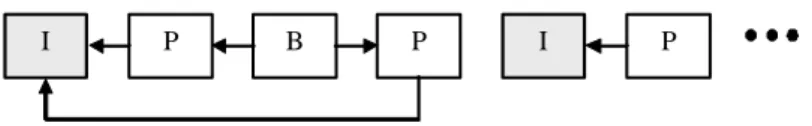
Figure 2.5: An example reference structure in video coding
2.6.2
Video Compression Principles
Current video compression techniques achieve significant bit rate savings by com-bining still image compression and motion compensation. The motivation behind the use of image and video compression is the huge amount of raw data that em-anates after the video capture. For example a raw video of resolution 1280x720 at 30 fps requires nearly 650Mbps which is unattainable in current technology for commercial use. The most recent compression standard H.264 can reduce the bit rate down to 10 Mbps with a reasonable quality.
A generic referencing structure of a video codec is given in Figure 2.5. The frames denoted with I are intra coded frames, the other ones, P and B, are inter coded frames. Intra-coding refers to self-decodable frames that are still image coded. Inter coding refers to compressing the frame of interest dependent on the previous or subsequent frames. When a frame is compressed referring only to previous frames it is denoted with the letter P, and when it is coded bi-directionally referring to both previous and subsequent frames it is denoted with the letter B.
In the following sections we briefly describe the two different modes of video coding, namely intra and inter coding.
Intra Coding
Intra coding uses the principles of still image compression techniques such as the ones used in JPEG [19]. It starts with RGB yo YUV conversion, a simple linear
conversion, which removes the dependency in color representation of RGB. After the YUV conversion, 2-D DCT is applied on block-by-block basis (generally 8x8 or 16x16) in order to reduce the correlation among the image pixels. After DCT and quantization, zig-zag scan and entropy coding are used to apply the final compression steps to the chosen frame.
Intra coded frames are introduced on a regular basis in order to allow fast synchronization and prevention of the propagation of losses. The period of intra frames are subject to optimization for different types of environments. There is a significant tradeoff between bit rate, quality and error robustness on the period of intra frames. Since the entire frames between two intra-frames are eventually dependent on them, intra-frames are generally given the highest priority during lossy transmission.
Inter Coding
In the current block based video coding systems, inter coded frames are the main factor of bandwidth saving. Inter coding refers to the compression of frames by removing the temporal redundancy, whereas intra-coding removes the spatial re-dundancy. The simplest way of removing the temporal redundancy is by just sending the residual (the difference) between the current and the previous frame, however more compression can be achieved by means of estimating and com-pensating the motion between the frames. Block based motion estimation and compensation is considered to be the most practical and efficient technique for this purpose.
In Figure 2.6, block based motion estimation is presented. The aim of block based motion estimation is to find a motion vector that relates best matching block from the nth frame to the block of interest in the (n + 1)thframe. The best
Frame n Frame n+1 Search region MB of best match MB of interest (xa, ya) (xb, yb) (xa, ya) Motion vector
Figure 2.6: Block-based motion estimation in inter-frames
of the method. In Figure 2.6, an artificial motion vector is demonstrated that heads from the point (xa, ya) to (xb, yb). This process is repeated for each block
in the current frame. After all motion vectors are determined, a new motion compensated frame from the (n + 1)th frame is formed using the best matching
blocks of the nth frame. A residual frame is constructed by subtracting the
motion compensated frame from the nth frame, and the residual is still image
coded. Then, the still image coded residual together with the motion vectors are sent or stored as the compressed data of frame n + 1.
2.6.3
Video Streaming Principles
The term streaming appeared in the multimedia area following the possibility of on-demand or real-time video over the Internet. It refers to the display of the multimedia content at the end-user while it is being transmitted from the server.
In the lossy channels, video streaming is a complicated task where one has to deal with many problems, such as latency, packet loss detection and recovery, and bit rate budget-quality tradeoff, etc.. One of the most widely used stream-ing protocols is Hypertext Transfer Protocol (HTTP) over TCP [44], which is
a good choice to avoid firewall issues. Another protocol similar to HTTP is Real-Time Streaming Protocol (RTSP) [45] which is being adopted to many sys-tems. Real-time Transport Protocol (RTP) [46] is another streaming protocol which is essentially a packet format that adds a timestamp, a sequence number, a contributing source identifier, and a payload type and format on top of an ordinary TCP or User Datagram Protocol (UDP) packet. In these protocols, there are transmission rate control, congestion control, error control and packet loss recovery, due to the properties of TCP. However this may cause latency and inefficiency in bandwidth utilization.
RTP over UDP is another alternative to these systems where packets are sent once and there is no means of an integrated transmission rate control or error control. In these systems transmission rate and error controls can be performed by the application layer which brings flexibility. The best candidate for appli-cation layer error control in these systems is FEC, where few extra packets are inserted to recover any lost packets. Thus, RTP over UDP provides flexibility, lower latency and bandwidth utilization, which is well-suited for video streaming.
2.7
Multi-view Video Coding and Streaming
Multi-view video coding is an approach for the efficient compression and trans-mission of image sequences captured from more than one cameras. Due to the increase in the number of captured views, eventually, the raw bit rate increases linearly with the number of cameras. This fact necessitates the exploitation of spatial dependencies among the views, besides the exploitation of temporal de-pendencies among frames of one view. Standardization of multiview video is under process as a study in ISO/IEC [39], [40]. Other than the standardization effort, there are individual studies on multi-view coding [41], [42] and [43].
I P P B P P I P P P B P P P P P P B P P P P P P View 0 View 1 View 2
Figure 2.7: An example reference structure in multi-view video coding
In Figure 2.7, a referencing structure for multi-view coding is presented. Many different referencing structures can be constructed according to the need of ap-plication. Generally, one of the views is coded independent of the others (View 0 in Figure 2.7) in order to provide compatibility to monoscopic decoders. Other views are coded dependent on their prior. In such a scheme, if one tries to group the frames according to their importance, the easiest way is to use the referencing structure. The priority of the frames diminishes from top to bottom. Providing different protection to different frames can increase the quality of the decoded multi-view video significantly.
Streaming of multi-view coded video is another research topic. In [47], a streaming system that uses standard LAN connection is proposed. In [48], the multi-view coded video is transmitted over RTP/UDP. Another study is on the utilization of DCCP for streaming [49]. In [50], stereoscopic video is layered using data partitioning, but an FEC method specific to stereoscopic video is not used. The video data is segmented into three parts, however only the part containing motion and disparity compensated error residuals is protected with different channel code rates to observe changes experimentally, and simply, the significance of UEP over EEP is demonstrated.
2.8
Error Resilient Video Streaming with
Foun-tain Codes
Fountain codes for error resilient video streaming have gained a significant in-terest in recent years. This is mainly caused by the extreme increase in the transmission bit rates due to widespread deployment of video streaming systems and consequent reliability issues. Fountain codes promise reliability with low complexity for this large amount of data.
A scalable video streaming system which uses Raptor codes using multiple media servers is presented in [51]. Different servers with different channel char-acteristics stream same scalable video content independent of the client. The authors considered delivery of two layers; base layer and enhancement layer. They proposed two schemes: one with optimal rate allocation with complete knowledge of network condition, and the other one with an heuristic approach. A unicast video streaming method with rateless codes is proposed in [52]. Con-trary to the idea of rateless codes, an acknowledgement message is sent from the receiver for every source block. Thus, redundant output symbols arrive to the receiver before the acknowledgement arrives to the sender. The authors derive strategies to minimize the overhead under lossy transmission. A multi-layered video coding scheme with unequal error protection with rateless codes are proposed in [53]. A layer-aware FEC (L-FEC) system which applies differ-ent protection to the defined dependdiffer-ent layers by a combined FEC scheme is proposed. FEC is applied according to the dependency of the layers, so that the FEC of current layer is created using all layers up to current layer. Foun-tain codes also attracted interest for video transmission in mobile and ad hoc networks. In [54], the authors used Scalable Video Coding (SVC) for rate adap-tation at the peers of a mobile network. They also used application layer FEC
utilization of SVC and AL-FEC allows distributed reception of video between the peers. Another work about rateless codes in mobile networks is presented in [55]. The authors proposed a new UEP structure for Raptor codes where they apply different code rates in the pre-coding stage to the video content with different priorities. The authors proposed the scheme for scalable video delivery in mobile networks. In [56], authors propose layered video streaming system, where the most important layers received highest protection. The proposed system for SVC is suitable for devices with limited computation capability. Network coding with video streaming, which targets the case of several servers and clients, is another novel research area. In [57], the authors proposed an efficient video transmission scheme by combining Raptor codes and network coding. Rateless codes are also used for energy-efficient video streaming studies, such as in [58].
2.9
Improving the State-of-the-Art Techniques
Fountain codes, especially Raptor codes, are the state-of-the-art error correc-tion scheme for PEC. They appear in the most recent standards for multimedia broadcast, such as Digital Video Broadcast for Hand-held (DVB-H) [14] and 3rd
Generation Partnership Project (3GPP) [15]. In our work, we analyze and model the performance of LT and Raptor codes which can be used in these multime-dia broadcast systems for ease of performance monitoring and optimization of quality.
Studies on the state-of-the-art multi-view video codecs are carried on under ISO/IEC [39], [40]. Integration of this system with an FEC scheme is one of the possible ways to improve the standard for handling the lossy transmission. Moreover, UEP techniques can also be applied since multi-view video has a high number of data groups with different loss sensitivities. In this sense, we study on the transmission of layered stereoscopic video with FEC.
Chapter 3
Error Correction in Stereoscopic
Video Streaming
3.1
Motivation
Video streaming is a challenging problem when the transmission medium is lossy. Especially, when the dimension of the video increases the problem becomes more complicated. We aim at optimizing the visual quality of stereoscopic video under lossy transmission. In order to achieve this, we suggest a method for modeling the end-to-end rate distortion characteristics of video streaming. Specifically, we propose a system that models the RD curve of video encoder and performance of channel codec to jointly derive the optimal encoder bit rates and unequal error protection (UEP) rates specific to the layered stereoscopic video streaming.
In Section 3.2, we present common error resiliency tools and demonstrate that in order to achieve best quality, FEC is required for lossy transmission. In Section 3.3, we give an overview of the stereoscopic streaming system. In Section 3.4, we provide the calculation of the RD curve for the three layers of
encoder distortion minimization. In Section 3.5, we provide the performance modeling of Raptor codes that is further detailed in Section 4.5.4. In Section 3.6, we calculate the approximate distortion in video quality when units of video data are lost during transmission. Finally, in Section 3.7, we perform end-to-end distortion minimization to obtain optimal video encoder bit rates and UEP bit rates, and provide simulation results under various transmission scenarios.
3.2
Basics of Error Resiliency Techniques for
Video Streaming
Error resiliency in video streaming refers to the techniques that aim at improving the quality of the video in case of packet losses during the transmission. In order to define the quality of the monoscopic video, generally peak signal to noise ratio (PSNR) measure, which is defined as
P SN R = 10 log á 2B− 1¢2 MSE ! , (3.1)
is used, where B is the number of bits per pixel (generally 8), and MSE is mean squared error between the original and reconstructed T images of size m by n. The MSE is defined as
MSE = 1 T T −1 X t=0 1 mn m−1X i=0 n−1 X j=0
kIorig(i, j, t) − Irec(i, j, t)k2 , (3.2)
where Iorig(i, j, t) and Irec(i, j, t) are the pixel values at the location (i, j) of the
tth frame of original and reconstructed frames, respectively. This PSNR measure
will be used in Sections 3.2.1 to 3.2.3, in order to demonstrate the effect of the error resiliency schemes in the case of monoscopic video. The PSNR measure that we use for the quality measurement of stereoscopic video is defined in (3.28).
Frame n (a)
Frame n Frame n+1
(b)
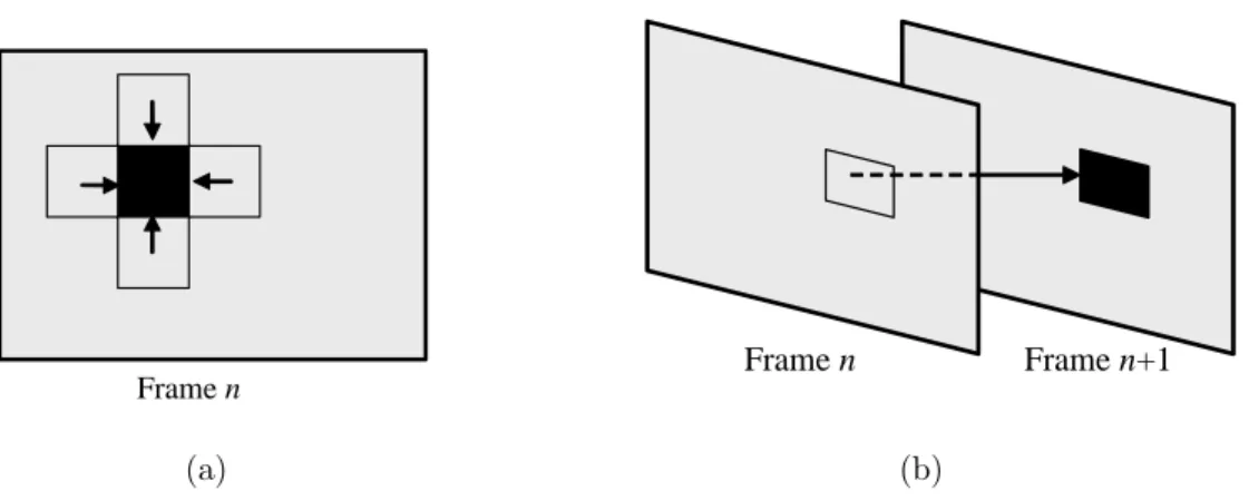
Figure 3.1: The representation of two basic error concealment techniques, (a) spa-tial, (b) temporal
3.2.1
Error Concealment
One of the most commonly used error resiliency techniques is error concealment. In this technique, the lost packet, namely some part of the image in the sequence, is replaced with an accurate representation from the neighboring received parts of the video. In Figure 3.1, two basic error concealment techniques are presented: spatial and temporal. The black block represents the lost part of the frame. In Figure 3.1(a), it is concealed by the average of neighboring blocks, whereas in Figure 3.1(b) concealed by the co-located block in the previous frame. There are many studies on advanced error concealment techniques such as described in [59], [60], [61].
The effect of error concealment on the quality of received video is signifi-cant. In Figure 3.2, the reconstructed video quality measures after %1, %3 and %5 losses with error concealment and the reconstructed video quality after %1 loss without error concealment are demonstrated with the reference software of H.264/AVC given in [62] for the ‘Rena’ video described in Section 3.7.2. Even at %1 loss, the quality of the video decreases significantly when error concealment is not used. The technique for error concealment is simply replacing the lost part of the video with the previous frame, namely temporal concealment. Error
0 0.5 1 1.5 2 2.5 3 3.5 4 x 10⁵ 15 20 25 30 35 40 45 50 Bit rate (bps) PSNR (dB) No−Loss %1 Loss, EC %3 Loss, EC %5 Loss, EC %1 Loss, no EC
Figure 3.2: The results on the effect of error concealment on video quality concealment is generally independent of the encoder, however for better gains the video has to be encoded in small sized slices (NAL units).
3.2.2
Flexible Macroblock Ordering
Flexible macroblock ordering (FMO) is another error resiliency tool that enables the division of image sequences into different regions called slice groups, which may consist of several slices (NAL units). Each slice group is encoded inde-pendently and this yields more efficient error concealment by exploiting spatial redundancy. When the slice groups are chosen so that no neighboring blocks remain in the same group, a lost slice can be more accurately concealed using the neighboring slices. There are many studies on different FMO schemes, such as the ones described in [21], [20], [63].
In Figure 3.3, we give the results when FMO is used on top of error con-cealment. The video is encoded and decoded with the reference software of H.264/AVC in [62] for the ‘Rena’ video described in Section 3.7.2. The chosen