A Chebyshev Polynomial Approach for High-Order Linear Fredholm-Volterra Integro-Differential Equations

(1)

GU J Sci

25(2):393-401 (2012)

ORIGINAL ARTICLE

♠

Corresponding author, e-mail: ngamze@mu.edu.tr

A Chebyshev Polynomial Approach for High-Order

Linear Fredholm-Volterra Integro-Differential

Equations

Gamze YÜKSEL

♠,1

, Mustafa GÜLSU

1

, Mehmet SEZER

1

Department of Mathematics, Faculty of Science, Mugla University, Mugla, Turkey

Received:06/06/2010 Revised: 24/11/2010 Accepted:27/02/2011 ABSTRACT

The purpose of this study is to present a method for solving high order linear Fredholm-Volterra integro-differential equations in terms of Chebyshev polynomials under the mixed conditions. The method is based on the approximation by the truncated Chebyshev series. The higher order linear Fredholm-Volterra integro-differential equations and the conditions are transformed into the matrix equations, which corresponds to a system of linear algebraic equations with the unknown Chebyshev coefficients. Combining these matrix equations and then solving the system yields the Chebyshev coefficients of the solution function. Finally, the effectiveness of the method is illustrated in several numerical experiments and error analysis is performed.

Keywords: Chebyshev polynomials, Fredholm-Volterra integral equations, Polynomial approximations

1. INTRODUCTION

Many mathematical formulations of physical phenomena contain Fredholm and Volterra integro-differential equations (FVIDE). These equations arise in fluid dynamics, biological models, chemical kinetics and etc. Finding the exact solution of FVIDE is generally difficult, even impossible. Therefore, it is needed to obtain the approximate solutions. Several numerical methods have been used such as the successive approximation method for FVIDE [1-17]. On the other hand, in recent years, the matrix method has been developed for solving the linear Fredholm-Volterra integral equations. For example, the method is used for solving a system of differential equations [18] and differential-algebraic equations [19]. Also, the method is applied to one-dimensional Volterra integral and integro-differential equations [20-22].

The aim of the presented paper is to apply the Chebyshev method for solving high order linear Fredholm-Volterra integral equations. The method is referred to as the Chebyshev collocation method. Chebyshev polynomials are well known family of

orthogonal polynomials on the interval [ 1,1]- . These polynomials present, among others, very good properties in the approximation of functions. Therefore, Chebyshev polynomials appear frequently in several fields of mathematics, physics and engineering [23,24]. 2. Definition of the problem

Let us consider the high order linear Fredholm-Volterra integral equations as follows,

1 ( ) 1 0 1 2 1 ( ) ( ) ( ) ( , ) ( ) ( , ) ( ) m k k f k x v P x y x g x K x t y t dt K x t y t dt l l = -= + +

å

ò

(1) under the mixed conditions

åå

-= =

=

1 0 0 ) (

)

(

m k r j i j k k ij

y

c

m

,

i

=

0 ,

1 ,...,

m

-

1

,

1 c

_j

1 - £

£

(2)

where

y x

( )

is an unknown function,

g x

( )

,

P x

_k

( )

and

K x t

( , )

are defined on an interval

1 x t

,

1 - £

£

, also

c c

ijk

,

j are constants.

We will find the approximate solution of (1) by means of the Chebyshev polynomials such that

å

=

N n n n

T

x

a

x

y

0

)

(

'

)

(

,

)

cos

cos(

)

(

x

n

1

x

T

n

-=

, -1£x£ 1 (3) where

a

_n

,

n

=

0,1, 2,...,

N

are the Chebyshev coefficients to be determined and N is chosen any positive integer such that

N

³

m

.

We choose the collocation points as the extremes of the Chebyshev polynomials

T x

_r

( )

cos

,

0,1,...,

s

N

s

x

s

N

-æ

ö

=

_ç

_÷

p

=

è

ø

. (4)

2.1. The fundamental relations Let us write Eq. (1) in the form

)

(x

D

=

g

(x

)

+

l

₁

I

_f

(x

)

+

l

₂

I

_v

(x

)

(5) where the differential part

)

(x

D

=

å

= m k k k

x

y

x

P

0 ) (

)

(

)

(

(6)

Fredholm and Volterra integral part respectively,

ò

-=

1 1

)

(

)

,

(

)

(

x

K

x

t

y

t

dt

I

_f _f (7) and 1

( )

( , ) ( )

x v v

I x

K x t y t dt

-=

_ò

. (8) We convert these parts and the mixed conditions (2) to the matrix forms in the following sections.

2.2. Matrix relation for the differential part

We first consider the approximate solution

y x

( )

of Eq. (1) defined by the truncated Chebyshev series (3). Then we can put expression (3) in the matrix form

( )

y x

= T

x

A

(9) where 0 1

[ ( )

T x T x

( ) ...

T x

_n

( )]

=

T( )

x

and 0 1

[1/ 2

...

]

A

=

a a

a

N T.

On the other hand, there is a relation between the matrix

( )

T x

and its derivative

T

(1)

( )

x

is

( )

x

=

( )

x

(1) T

T

J

where

The second derivative of

T

( )

x

as follows,

( 2) (1)

( )

x

=

( )

x

T

=

( )

x

T 2

T

J

T

(J )

Hence, we obtain the following formula for

k th

derivatives of

T

( )

x

:

( )k

_{( )}

_x

=

(k-1)

_{( )}

_x

T

=

_{( )}

_x

T k

T

(J )

T

(J )

(10)

The matrix form of the kth derivatives of function

( )

y x

is obtained as follows ( )

( )

k

y

x

=

T

x

(J ) A

T k (11) By substituting the equation (11) into equation (6), we obtained the matrix representation of the differential such that k 0

( )

m T k k

x

=

å

P ( )T( )(J ) A

D

(12)

2.3. Matrix relation for the Fredholm integral part

Let us assume that the kernel function

K x t

( , )

can be expanded to univariate Chebyshev series with respect to

t

as follows ' ' 0 0

( , )

( ) ( )

N N ls l s l s

K x t

k T x T t

= =

=

å å

,

N

s

l

,

=

0 ,

1 ,...,

(13) in which a summation symbol with double primes denotes a sum with first and last terms halved. Then the

matrix equation of the kernel functions

)

,

( t

x

K

f becomes ) 1 ( ) 1 ( 0 2 2 0 2 0 0 2 0 2 0 2 0 0 0 2.5 0 2.5 0 5 0 0 0 2.4 0 2.4 0 0 0 0 0 2.3 0 3 0 0 0 0 0 2.2 0 0 0 0 0 0 0 1 0 0 0 0 0 0 0 + + ú ú ú ú ú ú ú ú ú ú ú ú û ù ê ê ê ê ê ê ê ê ê ê ê ê ë é = N x N N N N N N N N L L M M O M M M M M L L L L L L J

(3)

GU J Sci, 25(2):393-401 (2012)/ Gamze Yüksel, Mustafa Gülsu, Mehmet Sezer

395 )

(

)

(

)

,

(

x

t

x

t

K

f

=

T

K

f

T

T ,

K

f

=

[

k

ls

]

(14) where

[ ]

00 01 0 10 11 1 0 1 1 1 1 4 2 2 1 2 1 2 N N ls N N NN k k k k k k k k k k é ù ê ú ê ú ê ú ê ú = ê ú ê ú ê ú ê ú ë û L L M M O M L 0 1

( )

[ ( )

( ) ...

( )]

T

x

=

T x T x

T x

_n 0 1

( )

[ ( )

( ) ...

( )]

T

t

=

T t T t

T t

_n

Substituting the Eq. (9) and Eq. (14) in the Fredholm integral part (7), we obtain fundamental matrix equations as follows 1 1 1 1 ( ) ( ) ( ) ( ) ( ) ( ) ( ) Q T K T T A T K T T A f T T f f f I x x t t dt x t t dt - -ì ü = = í ý î þ

ò

1 4 4 2 4 4 3 or shortly

( )

f

x

=

x

f f

I

T

K Q A

(15) In here, 1 1

( ) ( )

Q

f

T

t

T

t dt

-=

_ò

and

_Q

_[

_]

f

=

q

ij ,

( ,

i j

=

0,1,...,

N

)

where

2.4. Matrix relation for the Volterra integral part Similarly, let us assume that the kernel functions

( , )

v

K x t

can be expanded to univariate Chebyshev series with respect to

t

. Then the matrix form is obtained

( , )

( )

T

( )

v

x t

=

x

t

v

K

T

K T

,

K

_v

= ë û

é

k

v_ls

ù

(16) Substituting the Eq. (9) and Eq. (16) in the Volterra integral part (8), we have

1 1 ( ) ( ) ( ) ( ) ( ) ( ) ( ) ( ) v x x T T v v v x I x x t t x t t dt - -ì ü = = í ý î þ

ò

Q T K T T A T K T T A 1 4 4 2 4 4 3 or shortly,

( )

x

=

( )

x

_v _v

( )

x

I

_v

T

K Q

A

(17) In here, 1

( )

T

( ) ( )

T

x T v

Q x

t

t dt

-=

_ò

,

( )

[

( )]

Q

v v

x

=

q

ls

x

,

l

,

s

=

0 ,

1 ,...,

N

where 2 2 1 1 , 1 ( ) 1 ( ) 0 , ij l s odd l s l s q l s even ì ₊ ₊ ï - + -= í ï ₊ î

(

)

1 1 1 1 1 1 1 1 ( ) ( ) ( ) ( ) ( ) 2 ( ) ( ) ( ) ( ) 1 4 1 1 1 1 x x v ls l s l s l s x l s l s l s l s q x T t T t dt T t T t dt T t T t T t T t l s l s l s l s + -- -- + -+ -+ + -é ù = = + = ë û ì ü ï _- ₊ _- ï í _{+ +} _{+ -} _{- +} _{- -} ý ï ï î þ

ò

(4)

2.5. The fundemantal matrix equations

Now, substituting the collocation points (4) into (12), we obtain the fundamental matrix equations for the differential part as follows

T k 0

( )

m s k s s k

x

=

å

D

P ( )T( )(J ) A

or shortly T k 0 m k k=

=

å

D

P T(J ) A

(18) where 0 0 1 0 0 0 1 1 1 1 0 1 ( 1) ( 1) ( ) ( ) . . . ( ) ( ) ( ) . . . ( ) . . . . . . . . . . . . ( ) ( ) . . . ( ) N N N N N N N x N T x T x T x T x T x T x T x T x T x ₊ ₊ é ù ê ú ê ú ê ú = ê ú ê ú ê ú ê ú ê ú ë û T 0 1 ( 1) ( 1)

( )

0

0 ( )

0

0 (

)

k k k N N x N

P x

₊ ₊

é

ù

ê

ú

ê

ú

=

ê

ú

ê

ú

ë

û

L

M

O

M

L

k

P

Similarly, substituting the collocation points (4) into (15) as follows

)

( )

s s f f

x

= T

x

K Q A

f

I (

The fundamental matrix equation is obtained for Fredholm integral part such that,

f f

= TK Q A

f

I

(19) Where

K

_f

=

[

k

_lsf

]

, 00 01 0 10 11 1 0 1 1 1 1 4 2 2 1 2 1 2 N f N ls N N NN k k k k k k k k k k é ù ê ú ê ú ê ú ê ú é ù = ë û ê ú ê ú ê ú ê ú ë û L L M M O M L and

[

f

]

f

=

q

ij

Q

, 00 01 0 10 11 1 0 1 N N f ij N N NN q q q q q q q q q q é ù ê ú ê ú é ù = ë û ê ú ê ú ë û L L M M O M L

Finally, substituting the collocation points (4) into (17) as follows

( )

x

_s

=

( )

x

_s _v _v

( )

x

_s

I

_v

T

K Q

A

The fundamental matrix equation is obtained for Volterra integral part such that,

v v v

I

= TK Q A

(20) where 2 0 1 ( 1) ( 1)

( )

0 . . .

0

0 ( ) . . .

0 .

.

0

0 . . .

(

)

T

N _N _{x N}

T x

₊ ₊

é

ù

ê

ú

ê

ú

ê

ú

= ê

ú

ê

ú

ê

ú

ê

ú

ê

ú

ë

û

, 2 2 ( 1) ( 1) 0 . . . 0 0 . . . 0 . . . . . . . . . . . . 0 0 . . . K v v v v N x N K K K ₊ ₊ é ù ê ú ê ú ê ú = ê ú ê ú ê ú ê ú ê ú ë û

[

v

]

ls

k

=

v

K

, 00 01 0 10 11 1 0 1 1 1 1 4 2 2 1 2 1 2 N v N ls N N NN k k k k k k k k k k é ù ê ú ê ú ê ú ê ú é ù = ë û ê ú ê ú ê ú ê ú ë û L L M M O M L , 2 0 1 ( 1) ( 1)

( )

.

(

)

Q

v v v v N _N _{x N}

Q x

₊ ₊

é

ù

ê

ú

ê

ú

ê

ú

= ê

ú

ê

ú

ê

ú

ê

ú

ê

ú

ë

û

(5)

397

2.6. Matrix representation for the conditions The corresponding matrix form for the conditions (2) is obtained, by means of the Eq. (11) as follows

1 0 0

[

]

m r k ij j i k j

c

m

-= =

åå

T k

T( )(J ) A]=[

(21) where

i

=

0 ,

1 ,...,

m

-

1

.

3. METHOD OF THE SOLUTION

To obtain the approximate solution of high-order linear Fredholm-Volterra integro differential equation (1) with the mixed conditions (2) using the present method, we construct the fundamental matrix equations corresponding to Eq. (1) and Eq.(2). For this purpose, substituting the matrix relations (18), (19) and (20) into Eq.(1), we obtain the fundamental matrix equation as follows 1 2 0 m T k v _v k f f k=

-

=

å

P T(J ) A λ TK Q A λ TK Q A G

or shortly 1 2 0

)

m T k v _v k f f k=

ì

_-

ü

₌

í

ý

î

å

PT(J

λTK Q λ TK Q A G

þ

(22)

Denoting the expression in parenthesis of Eq. (22) by W, the fundamental matrix equation for Eq. (1) is reduced to

WA=G

(23) which corresponds to a system of

(

N

+

1)

linear algebraic equations with unknown Chebyshev coefficients

a a

₀

,

₁

,...,

a

_N. Similarly, the fundamental matrix equation for the mixed conditions (21) is reduced to

[

U; μ

i

] [

=

u

i0

u

i1

L

u

1N

;

m

_{i m N}

]

_´₍ ₊₁₎ ,

i

=

0,1,...,

m

-

1

Finally, to obtain the approximate solution of Eq. (1) under the mixed conditions (2), we replace the m rows of the augmented matrix

[

W;G

]

with the rows of the augmented matrix

[

U; μ

_i

]

. In this way, the Chebyshev coefficients are determined by solving the new linear algebraic system.

4. ACCURACY OF THE SOLUTION

We can easily check the accuracy of the method. Since the truncated Chebyshev series in (3) is an approximate solution of Eq. (1), it must be approximately satisfied this equation. Then, for each

x

= Î

x

_i

[ ]

a b

,

0,1, 2,...

i

=

0 )

(

)

(

)

(

)

(

)

(

x

i

=

D

x

i

-

1

I

f

x

i

-

2

I

v

x

i

-

g

x

i

@

E

l

If

max(10 )

ki

=

10

-k_{(k is any positive integer) is}

prescribed, then the truncation limit N is increased until the difference

E x

( )

_i at each of the points

x

_i becomes smaller than the prescribed

10

-k.

5. NUMERICAL EXAMPLES

In this section we apply the present method to the following problems. To show the efficiency of the present method, the approximate solutions are compared with the exact solutions and the other approximate solutions that are given in literature. Example 1: Let us consider the following problem

1 1 1 2 3 4 5 6

( )

(

) ( )

( )

27 41

1

3

1

3

5

20

2

4

5

x

y x

x t y t dt

xt y t dt

x

-

-¢ -

-

=

+

-

- -

-ò

ò

(24)

(0)

1 ,

1

1 y

=

- £ £

x

(25) To find the approximate solution of the problem with the present method, we choose the collocation points for

3 N

=

as follows

p

N

i

N

x

_i

=

cos

(

-

)

,

i

=

0,1, 2,3

, 0 1 2 3

1

1 1,

,

1

2

2 x

= -

x

= -

x

=

x

=

.

Hence, the fundamental matrix equation of the problem (24) is obtained as

{

T

}

1 f f v v

P TJ - TK Q - TK Q

A = G

.

The fundamental matrix equation for the initial condition (25) is obtained such that

[

]

(0)

1 0

y

=

-

= 1

T

A

m

It can be showed as matrix equation as follows,

[ ]

1

UA = λ

or augmented matrix form

[

U;λ

₁

] [

=

1 0

-

1 0 ; 1

]

. Hence, the new augmented matrix based on the condition as follows

(6)

2

53

143 435 ;

325 1316 2916 457192 9 20 ; 3293640

1316 7148 457192

14 ; 899128

1

0

1

0 ;

1 -é

ù

ê

_-

ú

ê

ú

é

ù=

ë

_{û ê}

_-

_ú

ê

_-

ú

ë

û

W;G

%

Solving this system, the Chebyshev coefficients matrix is obtained as

[

5 2 15 4

3 2 1 4

]

T

=

A

Thereby the solution of the given problem becomes 3 1 1 2 2 3 3 0 2 3 3 1 ( ) ' ( ) ( ) ( ) ( ) ( ) 2 5 15 3 1 (2 1) (4 3 ) 2 4 2 4 ( 1) n n o o n y x a T x a T x aT x a T x a T x x x x x x = = = + + + = + + - + -= +

å

which is the exact solution.

Example 2: Let us consider the problem

( )

( ) 2 ( )

cos( ) 3sin

(0)

0,

(0)

1 y x

xy x

y x

x

y

¢¢

+

¢

-

=

-¢

=

which has the exact solution

y x

( )

=

sin

x

. The fundamental matrix equation of this problem becomes

{

T 2 T T 0

}

2 1 0

P T(J ) + P TJ + P T(J )

A = G

.

The approximate solutions of this problem for N=9

8 8 2 3 7 4 5 7 6 7 7 8 5 9 ( ) 0.1310000310 0.999999994 0.6197730410 0.166666637 0.19482610 0.00833329742 0.5403496310 0.000198338298 0.71349849610 0.26387182110 y x x x x x x x x x x - -- -- -= + + - -+ + - -+

In Table1, we present the absolute errors obtained for different values of N. Also, the approximate solution and the exact solution are illustrated in Fig.1.

Table1. Absolute errors for Example 2

X Chebyshev Method N=4 Chebyshev Method N=7 Chebyshev Method N=9

-1 1.3062E-3 1.7 E-8 1.0 E-9

-0.8 1.1627E-3 3.8 E-8 1.0 E-9

-0.6 8.2993E-4 9.0 E-9 1.0 E-9

-0.4 3.8692E-4 1.2 E-8 2.0 E-9

-0.2 7.1202E-5 1.2 E-8 2.0 E-9

0 3.000E-10 9.9E-12 1.3 E-9

0.2 1.323E-4 1.4 E-8 0.0000

0.4 1.3725E-3 8.0 E-9 2.0 E-9

0.6 5.8190E-3 9.0 E-9 3.0 E-9

0.8 1.6930E-2 1.3E-6 1.0 E-9

1 3.9802E-2 8.5E-6 5.9 E-8

-1 -0.8 -0.6 -0.4 -0.2 0 0.2 0.4 0.6 0.8 1 -1 -0.8 -0.6 -0.4 -0.2 0 0.2 0.4 0.6 0.8 1 N=4 N=7 N=9 Exact Solution

(7)

399

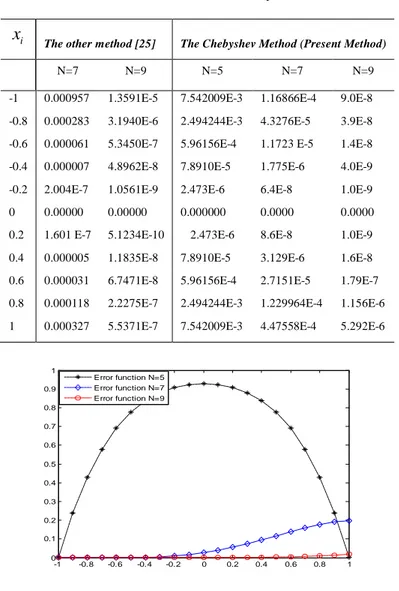
Example 3. Now consider the following fifth-order Fredholm integro differential equation

( 5 ) 2 ( 3 ) 1 2 1 ( ) ( ) ( ) ( ) cos( ) sin( ) ( ) y x x y x y x xy x x x x x y t d t -¢ - - - = - +

ò

In Table 2, we present a comparison for the absolute errors between the approximate solutions obtained by the present method with the method given by Akyüz [25].

It is clearly seen that, the present method has more accurate than the other method. In addition the error functions are illustrated in Fig.2.

with the conditions

( )

(0) 0, (0) 1,

(0) 0,

(0)

1,

iv

(0) 0

y

=

y

¢

=

y

¢¢

=

y

¢¢¢

=-

y

=

Table2. Absolute errors for Example 3

-1 -0.8 -0.6 -0.4 -0.2 0 0.2 0.4 0.6 0.8 1 0 0.1 0.2 0.3 0.4 0.5 0.6 0.7 0.8 0.9 1 Error function N=5 Error function N=7 Error function N=9

Figure 2. Error Analysis for Example 3

i

x

The other method [25] The Chebyshev Method (Present Method)

N=7 N=9 N=5 N=7 N=9

-1 0.000957 1.3591E-5 7.542009E-3 1.16866E-4 9.0E-8 -0.8 0.000283 3.1940E-6 2.494244E-3 4.3276E-5 3.9E-8 -0.6 0.000061 5.3450E-7 5.96156E-4 1.1723 E-5 1.4E-8 -0.4 0.000007 4.8962E-8 7.8910E-5 1.775E-6 4.0E-9 -0.2 2.004E-7 1.0561E-9 2.473E-6 6.4E-8 1.0E-9

0 0.00000 0.00000 0.000000 0.0000 0.0000

0.2 1.601 E-7 5.1234E-10 2.473E-6 8.6E-8 1.0E-9 0.4 0.000005 1.1835E-8 7.8910E-5 3.129E-6 1.6E-8 0.6 0.000031 6.7471E-8 5.96156E-4 2.7151E-5 1.79E-7 0.8 0.000118 2.2275E-7 2.494244E-3 1.229964E-4 1.156E-6 1 0.000327 5.5371E-7 7.542009E-3 4.47558E-4 5.292E-6

(8)

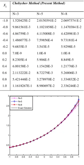
Example 4. Finally, let us consider the Volterra integro-differential equations 1 ( ) ( ) ( ) ( 1)sin sin( ) ( ) x x t y x xy x xy x e x x x e y t dt -¢¢ + ¢ - = - + +

_ò

with the conditions

y

(0) 1,

=

y¢

(0) 1

=

. The exact solution is

y x

( )

=

e

x.

In Table 4, the absolute errors are compared for

3,

5 N

=

N

=

and

N

=

8

. Also, the approximate

solutions and the exact solution are illustrated in Fig.3. In addition the error functions are plotted in Fig.4.

Table 3. Absolute errors for Example 4

i

x

Chebyshev Method (Present Method)

N=3 N=5 N=8

-1.0 1.520425E-2 2.0150391E-2 2.0697374 E-2 -0.8 9.861561E-3 1.1021858E-2 1.1470384 E-2 -0.6 4.86759E-3 4.115008E-3 4.420981E-3 -0.4 1.486077E-3 7.59856E-4 9.73181E-4 -0.2 9.6835E-5 3.543E-5 5.9298E-5

0.0 7.0E-9 1.0E-8 1.0E-8

0.2 8.2305E-4 5.906E-5 8.849E-5 0.4 6.00158E-3 1.15428E-3 1.21776E-3 0.6 2.113222E-2 8.72279E-3 5.26806E-3 0.8 5.421446E-2 3.278970E-2 1.334832E-2 1.0 1.1618267E-1 8.980697E-2 2.336246E-2

-1 -0.8 -0.6 -0.4 -0.2 0 0.2 0.4 0.6 0.8 1 0 0.5 1 1.5 2 2.5 3 N=3 N=5 N=8 Exact Solution

Figure 3. Comparison of the numerical results for Example 4 -1 -0.8 -0.6 -0.4 -0.2 0 0.2 0.4 0.6 0.8 1 0 0.2 0.4 0.6 0.8 1 1.2 1.4 1.6 1.8 Error function N=5 Error function N=7 Error function N=9

Figure 4. Error Analysis for Example 4 CONCLUSION

In this study, we present a new Chebyshev collocation scheme for the high order linear Fredholm-Volterra integro-differential equations. The method finds the truncated Chebyshev series solution satisfying (1) with the conditions (2) on the Chebyshev collocation nodes. The effectiveness of the method is illustrated in several numerical experiments. The method is very effective and simple. It doesn’t need to run high computer algorithms. There are more advantages of this method 1. This method is a direct method avoiding any iterative procedure.

2. It is observed that when the exact solution can be expanded to Chebyshev series, to get more accurate approximation, it should be taken more terms for Chebyshev approximate solutions. If N is chosen too large, more work than necessary will have been done. Also, there may be big computational errors. On the other hand, since collocation methods are not stable, the solution may not converge to the exact solution whenever

N

® ¥

. For this reasons, the truncation limit N should be chosen sufficiently large.

3. N th order approximation gives the exact solution when the solution is a polynomial and its degree equal to or less than N. If the solution is not a polynomial, it may get better result for sufficiently large N.

4. Since all finite ranges can be transformed to the interval [-1,1], this method can be applied to all finite ranges.

REFERENCES

[1] Y. Ren, B. Zhang, H. Qiao, “A simple Taylor-series expansion method for a class of second kind integral equations”, J. Comput. Appl.

Math. 110 (1999) 15–24.

[2] B. G. Pachpatta, “On mixed Volterra– Fredholm type integral equations”, Int. J.

(9)

401

[3] P. J. Kauthen, “Continuous time collocation methods for Volterra–Fredholm integral equations”, Num. Math. 56: 409–424(1989). [4] M. T. Rashed, “Lagrange interpolation to

compute the numerical solutions of differential, integral and integro-differential equations”, Appl. Math. Comput., 151 869-878(2004).

[5] Hashim, I. “Adomian decomposition method for solving BVPs for fourth-order integro-differential equations”, J. Comput. Appl.

Math. 193:658-664 (2006).

[6] Arikoglu, A., Ozkol, I. “Solution of boundary value problems for integro-differential equations by using differential transform method, Appl. Math. Comput., 168:1145-1158(2005).

[7] Maleknejad, K., Hadizadeh, M., “A new computational method for Volterra–Fredholm integral equations”, J. Comput. Appl. Math., 37:1–8 (1999).

[8] Wazwaz, A. M., “A reliable treatment for mixed Volterra–Fredholm integral equations”,

Appl. Math. Comput., 127:405–414(2002).

[9] Wazwaz, A. M., “A comparison study

between the modified decomposition method and the traditional methods”, Appl. Math.

Comput., 181:1703-1712(2006).

[10] Sweilam, N. H., “Fourth order integro-differential equations using variational iteration method”, Comput. Math. Appl., 54 1086-1091(2007).

[11] El-Sayed, S. M., Abdel-Aziz, M. R., “A comparison of Adomian's decomposition method and Wavelet-Galerkin method for integro-differential equations”, Appl. Math.

Comput., 136:151-159(2003).

[12] Maleknejad, K., Mahmoudi, Y., “Taylor Polynomial solution of high-order nonlinear Volterra_Fredholm integro-differential equations”, Appl. Math. Comput., 145 641-653(2003).

[13] Maleknejad, K., Mirzaee, F., Abbasbandy, S., “Solving linear integro-differential equations system by using rationalized Haar function method”, Appl. Math. Comput., 155:317-328(2005).

[14] A. Avudainayagam, C. Vani, “Wavelet-Galerkin method for integro-differential equations”, Appl. Num. Math., 32 247-254(2000).

[15] J. H. He, Variational iteration method: New development and applications, Comput.

Math. Appl., 54:881-894(2007).

[16] S. M. Hosseini, S. Shahmorad, Tau numerical solution of Fredholm integro-differential equations with arbitrary polynomial bases,

Appl. Math. Model., 27 :145-154(2003).

[17] E. L. Ortiz, L. Samara, An operational approach to the tau method for the numerical solution of nonlinear differential equations,

Computing, 27:15–25(1981).

[18] A. Akyüz and M. Sezer, Chebyshev polynomial solutions of systems of high-order linear differential equations with variable coefficients; Appl. Math. Comput. 144, 237-247(2003).

[19] A. Karamete, M. Sezer, “A Taylor collocation method for the solution of linear integro-differential equations”, Int. J. Comput. Math. 79 (9) :987–1000(2002).

[20] M. Sezer, Taylor polynomial solutions of Volterra integral equations, Int. J. Math.

Educ. Sci. Technol. 25 (5):625–633 (1994).

[21] M. Sezer, A method for approximate solution of the second order linear differential equations in terms of Taylor polynomials, Int.

J. Math. Educ. Sci.Tech. 27(6) 821–

834(1996).

[22] S. Nas, S. Yalçınbas, M. Sezer, “A Taylor polynomial approach for solving high-order linear Fredholm integro-differential equations”, Int. J. Math. Educ. Sci. Tech. 31 (2):213–225(2000).

[23] J. C. Mason, D. C. Handscomb , “Chebyshev Polynomials”, CRC Press ,(2003).

[24] A. G. Morris, T. S. “Horner, Chebyshev

polynomials in Numerical Analysi”,

Clarendon Pres, Oxford (1968).

[25] A. Akyüz, “A Chebyshev polynomial

approach for linear Fredholm-Volterra integro-differential equations in the most general form”, Appl. Math. Comput. 181:103-112(2006).