1Material Measurement Laboratory, National Institute of Standards and Technology, Gaithersburg, MD, USA. 2National Human Genome Research Institute, National Institutes of Health, Rockville, MD, USA. 3National Center for Biotechnology Information, National Library of Medicine, National Institutes of Health, Bethesda, MD, USA. 4Department of Human Genetics, University of California, Los Angeles, Los Angeles, CA, USA. 5Roche Sequencing Solutions, Belmont, CA, USA. 6Ontario Institute for Cancer Research, Toronto, Ontario, Canada. 7Charles-Bruneau Cancer Centre, Division of Hematology-Oncology, CHU Sainte-Justine, Montreal, Quebec, Canada. 8Molecular Biology Institute, University of California, Los Angeles, Los Angeles CA, USA. 9Department of Physiology and Biophysics, Institute for Computational Biomedicine, Weill Cornell Medicine, New York, NY, USA. 10The HRH Prince Alwaleed Bin Talal Bin Abdulaziz Alsaud Institute for Computational Biomedicine, Weill Cornell Medicine, New York, NY, USA. 11The WorldQuant Initiative for Quantitative Prediction, Weill Cornell Medicine, New York, NY, USA. 12The Feil Family Brain and Mind Research Institute, Weill Cornell Medicine, New York, NY, USA. 13Bionano Genomics, Inc., San Diego, CA, USA. 14Davies Research Centre, School of Animal and Veterinary Sciences, University of Adelaide, Roseworthy, SA, Australia. 1510× Genomics, Pleasanton, CA, USA. 16Broad Institute of Harvard and MIT, Cambridge, MA, USA. 17Google, Mountain View, CA, USA. 18Department of Computer Science, Roy G. Perry College of Engineering, Prairie View A&M University, Prairie View, TX, USA. 19Department of Genetics and Genomic Sciences, Icahn School of Medicine at Mount Sinai, New York, NY, USA. 20BC Cancer Genome Sciences Centre, Vancouver, British Columbia, Canada. 21Biomedical Genetics, Department of Medicine, Boston University Medical School, Boston, MA, USA. 22Pacific Biosciences, Menlo Park, CA, USA. 23Department of Computer Engineering, Bilkent University, Ankara, Turkey. 24Department of Computer Engineering, Konya Food and Agriculture University, Konya, Turkey. 25Departments of Computer Science and Biology, Johns Hopkins University, Baltimore, MD, USA. 26Department of Genetics, Harvard Medical School, Boston, MA, USA. 27Heinrich Heine University, Medical Faculty, Düsseldorf, Germany. 28Department of Bioinformatics and Computational Biology, MD Anderson Cancer Center, Houston, TX, USA. 29Department of Computer Science, Rice University, Houston, TX, USA. 30Bioinformatics R&D, Spiral Genetics, Seattle, WA, USA. 31Rutgers Cancer Institute of New Jersey, New Brunswick, NJ, USA. 32Department of Pathology, Robert Wood Johnson Medical School, New Brunswick, NJ, USA. 33Department of Computational Medicine and Bioinformatics, University of Michigan Medical School, Ann Arbor, MI, USA. 34Nabsys 2.0, LLC, Providence, RI, USA. 35Quantitative and Computational Biology, University of Southern California, Los Angeles, CA, USA. 36Joint Initiative for Metrology in Biology, SLAC National Accelerator Lab, Stanford University, Stanford, CA, USA. 37Human Genome Sequencing Center, Baylor College of Medicine, Houston, TX, USA. ✉e-mail: [email protected]
M
any diseases have been linked to SVs, most often defined as genomic changes at least 50 bp in size, but SVs are challenging to detect accurately. Conditions linked to SVs include autism1, schizophrenia, cardiovascular disease2,Huntington’s disease and several other disorders3. Far fewer SVs
exist in germline genomes relative to small variants, but SVs affect more base pairs, and each SV might be more likely to affect phe-notype4–6. Although next-generation sequencing technologies
can detect many SVs, each technology and analysis method has different strengths and weaknesses. To enable the community to
A robust benchmark for detection of germline
large deletions and insertions
Justin M. Zook
1✉, Nancy F. Hansen
2, Nathan D. Olson
1, Lesley Chapman
1, James C. Mullikin
2,
Chunlin Xiao
3, Stephen Sherry
3, Sergey Koren
2, Adam M. Phillippy
2, Paul C. Boutros
4,
Sayed Mohammad E. Sahraeian
5, Vincent Huang
6, Alexandre Rouette
7, Noah Alexander
8,
Christopher E. Mason
9,10,11,12, Iman Hajirasouliha
9, Camir Ricketts
9, Joyce Lee
13, Rick Tearle
14,
Ian T. Fiddes
15, Alvaro Martinez Barrio
15, Jeremiah Wala
16, Andrew Carroll
17, Noushin Ghaffari
18,
Oscar L. Rodriguez
19, Ali Bashir
19, Shaun Jackman
20, John J. Farrell
21, Aaron M. Wenger
22, Can Alkan
23,
Arda Soylev
24, Michael C. Schatz
25, Shilpa Garg
26, George Church
26, Tobias Marschall
27,
Ken Chen
28, Xian Fan
29, Adam C. English
30, Jeffrey A. Rosenfeld
31,32, Weichen Zhou
33,
Ryan E. Mills
33, Jay M. Sage
34, Jennifer R. Davis
34, Michael D. Kaiser
34, John S. Oliver
34,
Anthony P. Catalano
34, Mark J. P. Chaisson
35, Noah Spies
36, Fritz J. Sedlazeck
37and Marc Salit
36New technologies and analysis methods are enabling genomic structural variants (SVs) to be detected with ever-increasing accuracy, resolution and comprehensiveness. To help translate these methods to routine research and clinical practice, we devel-oped a sequence-resolved benchmark set for identification of both false-negative and false-positive germline large insertions and deletions. To create this benchmark for a broadly consented son in a Personal Genome Project trio with broadly available cells and DNA, the Genome in a Bottle Consortium integrated 19 sequence-resolved variant calling methods from diverse tech-nologies. The final benchmark set contains 12,745 isolated, sequence-resolved insertion (7,281) and deletion (5,464) calls ≥50 base pairs (bp). The Tier 1 benchmark regions, for which any extra calls are putative false positives, cover 2.51 Gbp and 5,262 insertions and 4,095 deletions supported by ≥1 diploid assembly. We demonstrate that the benchmark set reliably identifies false negatives and false positives in high-quality SV callsets from short-, linked- and long-read sequencing and optical mapping.
benchmark these methods, the Genome in a Bottle (GIAB) Consortium developed benchmark SV calls and benchmark regions for the son (HG002/NA24385) in a broadly consented and available Ashkenazi Jewish trio from the Personal Genome Project7, which
are disseminated as National Institute of Standards and Technology (NIST) Reference Material 83928,9.
Many approaches have been developed to detect SVs from differ-ent sequencing technologies. Microarrays can detect large deletions and duplications but not with sequence-level resolution10. Because
short reads (<<1,000 bp) are often smaller than or similar to the SV size, bioinformaticians have developed a variety of methods to infer SVs, including using split reads, discordant read pairs, depth of coverage and local de novo assembly. Linked reads add long-range (100+ kb) information to short reads, enabling phasing of reads for haplotype-specific deletion detection, large SV detection11–13
and diploid de novo assembly14. Long reads (>>1,000 bp), which
can fully traverse many more SVs, further enable SV detection, often sequence resolved, using mapped reads15,16, local assembly
after phasing long reads6,17 and global de novo assembly18,19. Finally,
optical mapping and electronic mapping provide an orthogonal approach capable of determining the approximate size and location of insertions, deletions, inversions and translocations while span-ning even very large SVs20–22.
GIAB recently published benchmark sets for small variants for seven genomes9,23, and the Global Alliance for Genomics and Health
Benchmarking Team established best practices for using these and other benchmark sets to benchmark germline variants24. These
benchmark sets are widely used in developing, optimizing and demonstrating new technologies and bioinformatics methods, as well as part of clinical laboratory validation12,15,25,26. Benchmarking
tool development has also been critical to standardize definitions of performance metrics, robustly compare variant call formats (VCFs) with different representations of complex variants and enable stratification of performance by variant type and genome context. Benchmark set and benchmarking tool development is even more challenging and important for SVs given the wide spectrum of types and sizes of SVs, the complexity of SVs (particularly in repetitive genome contexts) and that many SV callers output imprecise or imperfect breakpoints and sequence changes.
Several previous efforts have developed well-characterized SVs in human genomes. The 1000 Genomes Project catalogued copy number variants (CNVs) and SVs in thousands of individuals27,28. A
subset of CNVs from NA12878 was confirmed and further refined to those with support from multiple technologies using SVClassify29.
The unique collection of Sanger sequencing from the HuRef sam-ple has also been used to characterize SVs30,31. Long reads were
used to broadly characterize SVs in a haploid hydatidiform mole cell line32. The Parliament framework was developed to integrate
short and long reads for the HS1011 sample33. Most recently, the
Human Genome Structural Variation Consortium (HGSVC)6 and
the Genome Reference Consortium (GRC)34 used short, linked and
long reads to develop phased, sequence-resolved SV callsets, greatly expanding the number of SVs in three trios from 1000 Genomes, particularly in tandem repeats. Detection of somatic SVs in cancer genomes is a very active field, with numerous methods in devel-opment35–37. Although some of the problems are similar between
germline and somatic SV detection, somatic detection is compli-cated by the need to distinguish somatic from germline events in the face of differential coverage, subclonal mutations and impure tumor samples, among others38,39.
We build on these efforts by enabling anyone to assess both false negatives and false positives for a well-defined set of sequence-resolved insertions and deletions ≥50 bp in specified genomic regions. The HGSVC reported 27,622 SVs per genome but stated, in the Discussion, that “there is a pressing need to reduce the FDR of SV calling to below the current standard of 5%”6. The
Genome Reference Consortium developed SV calls in 15 individu-als from de novo assembly, but these assemblies were not haplo-type resolved and therefore missed some heterozygous variants34.
In addition, neither of these studies defined benchmark regions, which are critical in enabling reliable identification of false posi-tives. HGSVC provides a very valuable resource, allowing the com-munity to understand the spectrum of structural variation, but its lack of benchmark regions and its tradeoff of comprehensiveness for false positives limits its utility in benchmarking the performance of methods.
Our work in an open, public consortium is uniquely aimed at providing authoritative SVs and regions to enable technology and bioinformatics developers to benchmark and optimize their ods and to allow clinical laboratories to validate SV detection meth-ods. We developed methods and a benchmark set of SV calls and genomic regions that can be used to assess the performance of any sequencing and SV calling method. The ability to reliably identify false negatives and false positives has been critical to the enduring success of our widely adopted small variant benchmarks9,23. We
reached a similar goal for SVs by defining regions of the genome in which we are able to identify SVs with high precision and recall (here encompassing 2.51 Gb of the genome and 5,262 insertions and 4,095 deletions). Although we include SVs discovered only by long reads, we exclude regions with more than one SV, mostly in tandem repeats, as these regions are not handled by current SV comparison and benchmarking tools. In SV calls for the Puerto Rican child HG00733 from HGSVC6 and de novo assembly34 in
dbVar nstd152 and nstd162, respectively, we found that 24,632 out of 33,499 HGSVC calls and 10,164 out of 22,558 assembly-based calls were in clusters (within 1,000 bp of another SV call in the same callset). We also cluster calls by their specific sequence, improving upon previous work that clustered loosely by position, overlap or size. We address challenges in comparing calls with different rep-resentations in repetitive regions to enable the integration of a wide variety of sequence-resolved input callsets from different technolo-gies. Notably, we show that it correctly identifies false positives and false negatives across a diversity of technologies and SV callers. This is our principal goal: to make trustworthy assessment data and tools available as a common reference point for performance evaluation of SV calling.
Results
Candidate SV callsets differ by sequencing technology and anal-ysis method. We generated 28 sequence-resolved candidate SV
callsets from 19 variant calling methods from four sequencing tech-nologies for the Ashkenazi son (HG002), as well as 20 callsets each from the parents HG003 and HG004 (Supplementary Table 1). We integrated a total of 68 callsets, in which we define a ‘callset’ as the result of a particular variant calling method using data from one or more technologies for an individual. The variant calling methods included three small variant callers, nine alignment-based SV call-ers and seven global de novo assembly-based SV callcall-ers. The tech-nologies included short-read (Illumina and Complete Genomics), linked-read (10× Genomics) and long-read (Pacific Biosciences) sequencing technologies as well as SV size estimates from optical (Bionano Genomics) and electronic (Nabsys) mapping.
Figure 1 shows the number of SVs overlapping between our sequence-resolved callsets from different variant calling meth-ods and technologies for HG002, with loose matching by SV type within 1 kbp using SURVIVOR40. In general, the concordance
for insertions is lower than the concordance for deletions, except among long-read callsets, mostly because current short-read-based methods do not sequence resolve large insertions. This highlights the importance of developing benchmark SV sets to identify which callset is correct when they disagree and potentially when both are incorrect even when they agree.
Design objectives for our benchmark SV set. Our objective was
that, when comparing any callset (the ‘test set’ or ‘query set’) to the ‘benchmark set’, it reliably identifies false positives and false negatives. In practice, we aimed to demonstrate that most (ide-ally approaching 100%) of conflicts (both false positives and false negatives) between any given test set and the benchmark set were actually errors in the test set. This goal is typically challenging to meet across the wide spectrum of sequencing technologies and call-ing methods. Secondarily, to the extent possible, our goal was for the benchmark set to include a large, representative variety of SVs in the human genome. By integrating results from a large suite of high-throughput, whole-genome methods, each with their own sig-natures of bias, biases from any particular method are minimized. We systematically establish the ‘benchmark regions’ in this genome in which we are close to comprehensively characterizing SVs. We exclude regions from our benchmark if we could not reliably reach near-comprehensive characterization (for example, in segmental duplications). Notably, we demonstrate that the benchmark set is fit for purpose for benchmarking by presenting examples of com-parisons of SVs from multiple technologies and manual curation of discordant calls.
Benchmark set is formed by clustering and evaluating support for candidate SVs. We integrated all sequence-resolved candidate
SV callsets (‘Discovery callsets’ in Supplementary Table 1) to form the benchmark set, using the process described in Fig. 2. Because candidate SV calls often differ in their exact breakpoints, size and/or sequence change estimated, we used a new method called SVanalyzer (https://svanalyzer.readthedocs.io) to cluster calls esti-mating similar sequence changes. This new method was needed to account for differences in both SV representation (for example, dif-ferent alignments within a tandem repeat) and the precise sequence change estimated. Of the 498,876 candidate insertion and deletion calls ≥50 bp in the son-father-mother trio, 296,761 were unique after removing duplicate calls and calls that were the same when taking into account representation differences (for example, differ-ent alignmdiffer-ent locations in a tandem repeat). When clustering vari-ants for which the estimated sequence change was less than 20% divergent, 128,715 unique SVs remain. We then filtered to retain SV clusters supported by more than one technology and by five or more callsets from a single technology—Bionano or Nabsys. The 30,062 SVs remaining were then evaluated and genotyped in each member of the trio using svviz41 to align reads to reference and
alternate alleles from PCR-free Illumina, Illumina 6-kbp mate-pair,
haplotype-partitioned 10× Genomics and Pacific Biosciences with and without haplotype partitioning. We further filtered for SVs cov-ered in HG002 by eight or more Pacific Biosciences reads (mean coverage of about 60), with at least 25% of Pacific Biosciences reads supporting the alternate allele and consistent genotypes from all technologies that could be confidently assessed with svviz. This left 19,748 SVs. The number of Pacific Biosciences reads supporting the SV allele and reference allele for each benchmark SV is reported in Extended Data Fig. 1.
In our evaluations of these well-supported SVs, we found that 12,745 were isolated, whereas 7,003 (35%) were within 1,000 bp of another well-supported SV call. Upon manual curation, we found that the variants within 1,000 bp of another variant were mostly in tandem repeats and fell into several classes: 1) inferred complex variants with more than one SV call on the same haplotype; 2) inferred compound heterozygous variant with different SV calls on each haplotype; and 3) regions where some methods had the cor-rect SV call and others had inaccurate sequence, size or breakpoint estimates, but svviz still aligned reads to it because reads matched it better than the reference. We chose to exclude these clustered SVs from our benchmark set because methods do not exist to confi-dently distinguish between the above classes, nor do SV comparison tools exist for robust benchmarking of complex and compound SVs. Finally, to enable assessment of both false negatives and false positives, benchmark regions were defined using diploid assemblies and candidate variants. These regions were designed such that our benchmark variant callset should contain almost all true SVs within these regions. These regions define our Tier 1 benchmark set, which spans 2.51 Gbp and includes 5,262 insertions and 4,095 deletions. These regions exclude 1,837 of the 12,745 SVs because they were within 50 bp of a 20–49-bp indel; they exclude an additional 856 SVs within 50 bp of a candidate SV for which no consensus geno-type could be determined; and they exclude an additional 411 calls that were not fully supported by a diploid assembly as the only SV in the region. A large number of annotations are associated with the Tier 1 SV calls (for example, number of discovery callsets from each technology, number of reads supporting reference and alternate alleles from each technology and number of callsets with exactly matching sequence estimates), which enable users to filter to a more specific callset. We also define Tier 2 regions that delineate 6,007 additional regions in addition to the 12,745 isolated SVs, which are regions with substantial evidence for one or more SVs, but we could not precisely determine the SV. For the Tier 2 regions, multiple SVs within 1 kb or in the same or adjacent tandem repeats are counted as
0.0 0.2 0.4 0.6 0.8 1.0 Ratio of SV s a PacBio 10× Illumina CG PacBio 10× Illumina CG
CG Illumina 10× PacBio CG Illumina 10× PacBio
b
Fig. 1 | Pairwise comparison of sequence-resolved SV callsets obtained from multiple technologies and SV callers for SVs ≥50 bp from HG002. Heat
map produced by SURVIVOR40 shows the fraction of SVs overlapping between the individual SV caller and technologies split between (a) deletions and
(b) insertions. The color corresponds to the fraction of SVs in the caller on the x axis that overlap the caller on the y axis. Overall, we obtained a quite
Multiple assembly and variant calling methods
Benchmark regions pipeline
PacBio Illumina 250 bp Illumina mate-pair 10× Genomics Bionano
Benchmark calls pipeline
Clustered SVs supported by 2+ tech or 5+ callers or Bionano/Nabsys support
Benchmark set
Variant calling
Benchmark calls Excluding SVs within 1 kb of another SV
Genotyping with multiple technologies using svviz2 (Table 1)
Filtering SVs with consensus variant genotype across technologies for son Compare SVs 128,715 Discovery support 30,062 Evaluate/ genotype 19,748 Filter complex 12,745 Benchmark regions
Sequence-resolved SV calls were clustered using SVanalyzer merge within 20% edit distance SV calls discovered in 68 sequence-resolved callsets from four technologies for GIAB trio (Supplementary Table 1) Discovery 498,876 (296,761 unique) Nabsys De novo assembly
Fig. 2 | Process to integrate SV callsets and diploid assemblies from different technologies and analysis methods and form the benchmark set. The input
data sets are depicted in the center of the figure, with the benchmark calls and region pipelines to the left and right of the input data, respectively. The number of variants in each step of the benchmark calls integration pipeline is indicated in the white boxes. See Methods for additional description of the pipeline steps. Briefly, approximately 0.5 million input SV calls were locally clustered based on their estimated sequence change, and we kept only those discovered by at least two technologies or at least five callsets in the trio. We then used svviz with short, linked and long reads to evaluate and genotype these calls, keeping only those with a consensus heterozygous or homozygous variant genotype in the son. We filtered potentially complex calls in regions with multiple discordant SV calls, as well as regions around 20–49-bp indels, and our final Tier 1 benchmark set included 12,745 total insertions and deletions ≥50 bp, with 9,357 inside the 2.51 Gbp of the genome where diploid assemblies had no additional SVs beyond those in our benchmark set. We also define a Tier 2 set of 6,007 additional regions where there was substantial support for one or more SVs, but the precise SV was not yet determined.
a single region, so many SV callers would be expected to call more than 6,007 SVs in these regions.
Benchmark calls are well supported. The 12,745 isolated SV calls
had size distributions consistent with previous work detecting SVs from long reads6,15,17,26, with the clear, expected peaks for insertions
and deletions near 300 bp related to Alu elements and for insertions and deletions near 6,000 bp related to full-length LINE1 elements (Fig. 3). Note that deletion calls of Alu and LINE elements are most likely mobile element insertions in the GRCh37 sequence that are not in HG002. SVs have an exponentially decreasing abundance versus size if they fall in tandem repeats longer than 100 bp in the reference. Interestingly, there are more large insertions than large deletions in tandem repeats, despite insertions being more challeng-ing to detect. This is consistent with previous work detectchalleng-ing SVs from long-read sequencing15,17 and might result from instability of
tandem repeats in the bacterial artificial chromosome clones used to create the reference genome42.
When evaluating the support for our benchmark SVs, approxi-mately 50% of long reads more closely matched the SV allele for heterozygous SVs, and approximately 100% for homozygous SVs, as expected (Fig. 4a,c). Although short reads clearly supported and differentiated homozygous and heterozygous genotypes for many SVs, the support for heterozygous calls was less balanced, with a mode around 30%, and they did not definitively genotype 35% of deletions and 47% of insertions in tandem repeats because reads were not sufficiently long to traverse the repeat. These results high-light the difficulty in detecting SVs with short reads in long tandem repeats, as a sizeable fraction of reads containing the variant either map without showing the variant or fail to map at all. We also found high size concordance with Bionano (Fig. 4b,d). Because the region between Bionano markers can contain multiple SVs, the Bionano estimate will be the sum of all SVs between the markers, which can cause apparent differences in size estimates. For example, for insertions >300 bp where the Bionano Direct Label and Stain size estimate is >300 bp higher and >30% higher than the v0.6 inser-tion size, and where the entire region between Bionano markers is included in our benchmark bed, 23 out of the 40 Bionano insertions have multiple v0.6 insertions in the interval that sum to the Bionano size. In general, there was strong support from multiple technolo-gies for the benchmark SVs, with 90% of the Tier 1 SVs having sup-port from more than one technology.
For SVs on autosomes, we also identified if genotypes were consis-tent with Mendelian inheritance. When limiting to 7,973 autosomal
SVs in the benchmark set for which a consensus genotype from svviz was determined for both of the parents, only 20 violated Mendelian inheritance. Upon manual curation of these 20 sites, 16 were cor-rect in HG002 (mostly misidentified as homozygous reference in both parents due to lower long-read sequencing coverage); one was a likely de novo deletion in HG002 (17:51417826-51417932); one was a deletion in the T cell receptor alpha locus known to undergo somatic rearrangement (14:22918114-22982920); and two were insertions mis-genotyped as heterozygous in HG002 when in fact they were likely homozygous variant or complex (2:232734665 and 8:43034905). Extended Data Fig. 2 is a detailed contingency table of genotypes in the son, father and mother.
The GIAB community also manually curated a random subset of SVs from different size ranges in the union of all discovered SVs43.
When comparing the consensus genotype from expert manual curation to our benchmark SV genotypes, 627 of 635 genotypes agreed. Most discordant genotypes were identified as complex by the curators, with a 20–49-bp indel near an SV in our benchmark set, because they were asked to include indels 20–49 bp in size in their curation, whereas our SV benchmark set focused on SVs larger than 49 bp.
We compared the v0.6 Tier 1 deletion breakpoints to the deletion breakpoints from a different set of samples analyzed by HGSVC6 and GRC34. Of the 5,464 deletions in v0.6, (a) 45% had
breakpoints and 57% had size matching an HGSVC call; (b) 49% had breakpoints and 66% had size matching a GRC call; and (c) 58% had breakpoints and 73% had size matching either an HGSVC call or a GRC call. This comparison permitted 1-bp differences in the left and right breakpoints or 1-bp difference in size for any overlap, which ignores slight imprecision and off-by-one file format errors but does not account for all differences in representation within repeats. This high degree of overlap supports the base-level accu-racy of our calls and previous findings that many SVs are shared between even small numbers of sequenced individuals34.
We also evaluated the sensitivity of v0.6 to 429 deletions from the population-based gnomAD-SV v2.1 callset44 that were
homozy-gous reference in less than 5% of individuals of European ancestry, and at least 1,000 Europeans had the variant. Of these 429 deletions, 296 were in the v0.6 benchmark bed, and 286 of the 296 (97%) overlapped a v0.6 deletion. We manually curated the four deletions that had size estimates that were more than 30% different between gnomAD-SV and v0.6, and all were in tandem repeats and the v0.6 breakpoints were clearly supported by long-read alignments. We also manually curated the ten deletions that did not overlap a v0.6 deletion, which had homozygous reference frequencies in Europeans between 1.8% and 5%, and all ten were clearly homo-zygous reference in HG002, and nine of the ten were in our dis-covery callset and were genotyped as heterozygous in both parents but homozygous reference in HG002 (Supplementary Table 2). This demonstrates that, even though population-based callsets were not included in our discovery methods, v0.6 does not miss many com-mon SVs within the benchmark bed.
Benchmark set is useful for identifying false positives and false negatives across technologies. Our goal in designing this SV
benchmark set was that, when comparing any callset to our bench-mark VCF within the benchbench-mark BED file, most putative false positives and false negatives should be errors in the tested callset. To determine if we meet this goal, we benchmarked several call-sets from assembly-based and non-assembly-based methods that use short or long reads. Most of these callsets (‘Evaluation callsets’ in Supplementary Table 1) are different from the callsets used in the integration process by using different callers, new data types or new tool versions. We developed a new benchmarking tool truvari (https://github.com/spiralgenetics/truvari) to perform these com-parisons at different matching stringencies, because truvari enables
Alu Alu LINE
LINE
Alu Alu LINE
LINE
SVs overlapping tandem repeats >100 bp SVs not overlapping tandem repeats >100 bp
0 250 500 750 0 −10,000−7,500−5,000−2,500−1,000−750 −500 −250 0 250 500 750 1,0002,500 5,000 7,50010,000 500 1,000 1,500 SV length (bp) Count
Fig. 3 | Size distributions of deletions and insertions in the benchmark set.
Variants are split by SVs overlapping and not overlapping tandem repeats longer than 100 bp in the reference. Deletions are indicated by negative SV lengths. The expected Alu mobile elements peaks near ± 300 bp are indicated in blue, and LINE mobile elements peaks near ± 6,000 bp are indicated in orange.
users to specify matching stringency for size, sequence and/or dis-tance. We performed some comparisons requiring only that the variant size to be within 30% of the benchmark size and the posi-tion to be within 2 kb and some comparisons addiposi-tionally requir-ing the sequence edit distance to be less than 30% of the SV size. We compared at both stringencies because truvari sometimes could not match different representations of the same variant. An alterna-tive benchmarking tool developed more recently, which has more sophisticated sequence matching, is SVanalyzer SVbenchmark (https://github.com/nhansen/SVanalyzer/blob/master/docs/ svbenchmark.rst).
Upon manual curation of a random ten false-positive and false-negative insertions and deletions (40 total SVs) from each call-set being compared to the benchmark, nearly all of the false positives and false negatives were errors in each of the tested callsets and not errors in the GIAB callset (Fig. 5 and Supplementary Table 2). The version of the truvari tool we used could not always account for all differences in representation, so if manual curation determined that both the benchmark and test sets were correct, they were counted as correct. The only notable exception to the high GIAB callset accu-racy was for false-positive insertions from the Pacific Biosciences caller pbsv (https://github.com/PacificBiosciences/pbsv), for which
about half of the putative false-positive insertions were true inser-tions missed in the benchmark regions. This suggests that the GIAB callset might be missing approximately 5% of true inser-tions in the benchmark regions. When comparing Bionano calls to our benchmark, we also found one region with multiple inser-tions where our benchmark had a heterozygous 1,412-bp insertion at chr6:65000859, but we incorrectly called a homozygous 101-bp insertion in a nearby tandem repeat at chr6:65005337, when, in fact, there is an insertion of approximately 5,400 bp in this tandem repeat on the same haplotype as the 1,412-bp insertion, and the 101-bp insertion is on the other haplotype.
To evaluate the utility of v0.6 to benchmark genotypes, we also compared genotypes from two graph-based genotypers for short reads: vg45 and paragraph46. Of the 5,293 heterozygous and 4,245
homozygous variant v0.6 calls that had genotypes from both geno-typers, 3,642 heterozygous and 2,970 homozygous calls had identi-cal genotypes for vg, paragraph and v0.6. Also, 925 heterozygous and 496 homozygous variant v0.6 calls had genotypes that were different from both vg and paragraph. However, after filtering v0.6 calls annotated as overlapping tandem repeats, which are less accurately genotyped by short reads, only 326 heterozygous and 69 homozygous discordant genotypes remained. We manually curated SVs overlapping tandem repeats >100 bp
SVs not overlapping tandem repeats >100 bp
0.00 0.25 0.50 0.75 1.00
Long Short
Long Short
Fraction of reads supporting deletion
Read length a 100 1,000 1 × 10 3 1 × 10 4 1 × 10 5 3,000 10,000 30,000 1,000 10,000
Bionano deletion size
Deletion size
b
SVs overlapping tandem repeats >100 bp SVs not overlapping tandem repeats >100 bp
0.00 0.25 0.50 0.75 1.00
Long Short
Long Short
Fraction of reads supporting insertion
Read lengt h c 100 1,000 10,000
Bionano insertion size
Insertion size
d
Genotype 0/1 1/1
Fig. 4 | Support for benchmark SVs by long reads, short reads and optical mapping. Histograms show the fraction of Pacific Biosciences (long reads)
and Illumina 150-bp (short reads) reads that aligned better to the SV allele than to the reference allele using svviz, colored by v0.6 genotype, where blue is heterozygous and orange is homozygous. Variants are stratified into deletions (a) and insertions (c) and into SVs overlapping and not overlapping
tandem repeats longer than 100 bp in the reference. Vertical dashed lines correspond to the expected fractions 0.5 for heterozygous variants (blue) and 1.0 for homozygous variants (dark orange). The v0.6 benchmark set sequence-revolved deletion (b) and insertion (d) SV size is plotted against the size
estimated by Bionano in any overlapping intervals, where points below the diagonal (indicated by the black line) represent smaller sequence-resolved SVs in the overlapping interval.
ten randomly selected discordant heterozygous and homozygous genotype calls, and all ten heterozygous and all ten homozygous calls were correctly genotyped in v0.6 and were errors in short-read genotyping mostly in short tandem repeats, transposable elements or tandem duplications, demonstrating the utility of v0.6 for bench-marking genotypes. The ratio of heterozygous to homozygous sites in v0.6 is 3,433 to 2,031 for deletions and 3,505 to 3,776 for inser-tions, which is significantly lower than the ratio of approximately two for small variants, particularly for insertions. This difference likely results both from homozygous variants being easier to dis-cover and from tandem repeats that are systematically compressed in GRCh37, which result in homozygous insertions in our calls.
Technologies and variant callers have different strengths and weaknesses. Among the extensive candidate SV callsets that we
collected from different technologies and analyses, we found that certain SV types and sizes in our benchmark set were discovered by fewer methods (Fig. 6). In particular, more methods discov-ered sequence-resolved deletions than insertions; more methods discovered SVs not in tandem repeats; and most methods discov-ered deletions smaller than 1,000 bp not in tandem repeats. These results confirm the intuition that SV detection outside of repeats is simpler than within repeats and that deletions are simpler to detect than insertions because deletions do not require mapping to new sequence. Extended Data Fig. 3 further shows that the fewest SVs were missed by the union of all long-read discovery methods. The only exception was 50–99-bp deletions, which were all found by at least one short-read discovery method. Many insertions larger than 300 bp that were not discovered by any short-read method could be accurately genotyped in this sample by short reads. Interestingly, many deletions and insertions smaller than 300 bp that were not genotyped accurately by short reads were discovered by at least one short-read-based method. This likely reflects a limitation of the
heuristics we used for genotyping, which reduces the false-positive rate but might increase the false-negative rate. Both discovery and genotyping based on short reads had limitations for SVs in tandem repeats. These results confirm the importance of long-read data for comprehensive SV detection.
Sequence-resolved benchmark calls have annotations related to base-level accuracy. We provide sequence-resolved calls in our
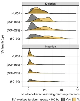
benchmark set to enable benchmarking of sequence change predic-tions. However, not all calls are perfect on a base level. When dis-covered SVs from multiple callsets have exactly matching sequence changes, we output the sequence change from the largest number of callsets. However, as shown in Fig. 7, not all benchmark SVs have calls that exactly matched between discovery callsets. For deletions not in tandem repeats, at least 99% of the calls had exact matches, but there were no exact matches for ~5% of deletions in tandem repeats, and, for large insertions, no exact matches existed for ~50% of the calls. This is likely because SVs in tandem repeats and larger insertions are more likely to be discovered only by methods using relatively noisy long reads.
Discussion
We integrated sequence-resolved SV calls from diverse technologies and SV calling approaches to produce a benchmark set enabling anyone to assess both false-negative and false-positive rates. This benchmark is useful for evaluating accuracy of SVs from a variety of genomic technologies, including short-, linked- and long-read sequencing technologies, optical mapping and electronic mapping. This resource of benchmark SVs, data from a variety of technologies and SVs from a variety of methods are all publicly available without embargo, and we encourage the community to give feedback and participate in GIAB to continue to improve and expand this bench-mark set in the future.
When developing this benchmark set, several tradeoffs were made. Most notably, we chose to exclude complex SVs and SVs for which we could not determine a consensus sequence. Limiting our set to isolated insertions and deletions removed approximately half of SVs for which there was strong support that some SV occurred. However, by excluding these complex regions from our SV bench-mark set, it enables anyone to use our sequence comparison-based benchmarking tools to confidently and automatically identify false False negative False positive
Long reads
Short reads
Deletion Insertion Deletion Insertion 0 10 20 30 40 0 30 60 90
Structural variant type
Count Is GIAB correct? No Maybe Partial Yes
Fig. 5 | Summary of manual curation of putative false positives and false negatives when benchmarking short and long reads against the v0.6 benchmark set. Most false-positive and false-negative SVs were
determined to be correct in the v0.6 benchmark (green), but some were partially correct due to missing part of the SV in the region (blue), were incorrect in v0.6 (black) or were in difficult locations where the evidence was unclear (orange).
Larger than 1,000 bp Smaller than 1,000 bp
Deletion Insertion 0 20 40 60 0 20 40 60 0.00 0.25 0.50 0.75 1.00 0.00 0.25 0.50 0.75 1.00
Number of discovery methods
Inverse cumulative distribution
SV overlaps tandem repeats >100 bp No Yes
Fig. 6 | Inverse cumulative distribution showing the number of discovery methods that supported each SV. All 68 callsets from all variant calling
methods and technologies in all three members of the trio are included in these distributions. SVs larger than 1,000 bp (top) are displayed separately from SVs smaller than 1,000 bp (bottom). Results are stratified into deletions and insertions and into SVs overlapping (dashed) and not overlapping (solid) tandem repeats longer than 100 bp in the reference. The gray horizontal line at 0.5 was added to aid comparison between panels.
positives and false nagatives at different matching stringencies (for example, matching based on SV sequence, size, type and/or geno-type). Bionano also identified large heterozygous events outside the benchmark regions, and future work will be needed to sequence resolve these large unresolved complex events, often near segmental duplications. In addition to our standard Tier 1 benchmark set, we also provide a set of Tier 2 regions in which we found substantial evidence for an SV but it was complex or we could not determine the precise SV. We also exclude regions from our benchmark set around putative indels (20–49 bp in size), which minimizes unreli-able putative false-negative and false-positive SVs around clustered indels or variants just under or above 50 bp.
Our benchmark also currently does not include more compli-cated forms of structural variations, including inversions, dupli-cations (except for calls annotated as tandem duplidupli-cations), very large copy number variants (v0.6 contains only one deletion and one insertion >100 kb), calls in segmental duplications, calls in tan-dem repeats greater than 10 kbp or translocations. This benchmark does not enable performance assessment of inversion detection (for example, with Strand-seq47) or in highly repetitive regions like
seg-mental duplications, telomeres and centromeres that are starting to be resolved by ultra-long nanopore reads48. We also do not
explic-itly call duplications, although in practice our insertions frequently are tandem duplications, and we have provisionally labeled them as such using SVanalyzer svwiden in the REPTYPE annotation in the benchmark VCF. Future work in GIAB will use new technolo-gies and analysis methods to include new SV types and more chal-lenging SVs. When using our current benchmark, it is critical to understand that it does not enable performance assessment for all SV types nor the most challenging SVs.
GIAB is currently collecting new candidate SV callsets for GRCh37 and GRCh38 from new data types (for example, Strand-seq47, Pacific Biosciences Circular Consensus Sequencing26
and Oxford Nanopore ultra-long reads49), new and updated SV
callers and new diploid de novo assemblies. We are also refining
the integration methods (for example, to include inversions) and developing an integration pipeline that is easier to reproduce. In the next several months, we plan to release improved benchmark sets for GRCh37 and GRCh38, using these new methods similarly to how we have maintained and updated the small variant callsets for these samples over time. We will also use the reproducible integra-tion pipeline developed here to benchmark SVs for all seven GIAB genomes. We will continue to refine these methods to access more difficult SVs in more difficult regions of the genome. Finally, we plan to develop a manuscript describing best practices for using this benchmark set to benchmark any other SV callset, similar to our recent publication for small variants24, with refined SV comparison
tools and standardized definitions of performance metrics. We have summarized the limitations of the v0.6 benchmark in Extended Data Fig. 4.
Online content
Any methods, additional references, Nature Research report-ing summaries, source data, extended data, supplementary infor-mation, acknowledgements, peer review information; details of author contributions and competing interests; and statements of data and code availability are available at https://doi.org/10.1038/ s41587-020-0538-8.
Received: 16 July 2019; Accepted: 28 April 2020; Published online: 15 June 2020
References
1. Sebat, J. et al. Strong association of de novo copy number mutations with autism. Science 316, 445–449 (2007).
2. Merker, J. D. et al. Long-read genome sequencing identifies causal structural variation in a Mendelian disease. Genet. Med. 20, 159–163 (2018). 3. Mantere, T., Kersten, S. & Hoischen, A. Long-read sequencing emerging in
medical genetics. Front. Genet. 10, 426 (2019).
4. Roses, A. D. et al. Structural variants can be more informative for disease diagnostics, prognostics and translation than current SNP mapping and exon sequencing. Expert Opin. Drug Metab. Toxicol. 12, 135–147 (2016).
5. Chiang, C. et al. The impact of structural variation on human gene expression. Nat. Genet. 49, 692–699 (2017).
6. Chaisson, M. J. P. et al. Multi-platform discovery of haplotype-resolved structural variation in human genomes. Nat. Commun. 10, 1784 (2019). 7. Ball, M. P. et al. A public resource facilitating clinical use of genomes.
Proc. Natl Acad. Sci. USA 109, 11920–11927 (2012).
8. Zook, J. M. et al. Extensive sequencing of seven human genomes to characterize benchmark reference materials. Sci. Data 3, 160025 (2016). 9. Zook, J. M. et al. An open resource for accurately benchmarking small
variant and reference calls. Nat. Biotechnol. 37, 561–566 (2019).
10. Sebat, J. et al. Large-scale copy number polymorphism in the human genome.
Science 305, 525–528 (2004).
11. Spies, N. et al. Genome-wide reconstruction of complex structural variants using read clouds. Nat. Methods 14, 915–920 (2017).
12. Marks, P. et al. Resolving the full spectrum of human genome variation using Linked-Reads. Genome Res. 29, 635–645 (2019).
13. Karaoglanoglu, F. et al. VALOR2: characterization of large-scale structural variants using linked-reads. Genome Biol. 21, 72 (2020).
14. Weisenfeld, N. I., Kumar, V., Shah, P., Church, D. M. & Jaffe, D. B. Direct determination of diploid genome sequences. Genome Res. 27,
757–767 (2017).
15. Sedlazeck, F. J. et al. Accurate detection of complex structural variations using single-molecule sequencing. Nat. Methods 15, 461–468 (2018).
16. Cretu Stancu, M. et al. Mapping and phasing of structural variation in patient genomes using nanopore sequencing. Nat. Commun. 8, 1326 (2017). 17. Chaisson, M. J. P. et al. Resolving the complexity of the human genome using
single-molecule sequencing. Nature 517, 608–611 (2014).
18. Chin, C.-S. et al. Phased diploid genome assembly with single-molecule real-time sequencing. Nat. Methods 13, 1050–1054 (2016).
19. Koren, S. et al. De novo assembly of haplotype-resolved genomes with trio binning. Nat. Biotechnol. https://doi.org/10.1038/nbt.4277 (2018). 20. Kaiser, M. D. et al. Automated structural variant verification in human
genomes using single-molecule electronic DNA mapping. Preprint at
https://www.biorxiv.org/content/10.1101/140699v1.full (2017). 21. Lam, E. T. et al. Genome mapping on nanochannel arrays for structural
variation analysis and sequence assembly. Nat. Biotechnol. 30, 771–776 (2012). Insertion Deletion 0 20 40 60 (50−99) (100−299) (300−999) >1,000 (50−99) (100−299) (300−999) >1,000
Number of exact matching discovery methods
SV length (bp)
SV overlaps tandem repeats >100 bp Yes No
Fig. 7 | Fraction of SVs for each number of discovery callsets that estimated exactly matching sequence changes. Variants are stratified into
deletions (top) and insertions (bottom) and into SVs overlapping (black) and not overlapping (gold) tandem repeats longer than 100 bp in the reference. SVs are also stratified by size (y axis) into 50–99 bp, 100–299 bp, 300–999 bp and 1,000 or more bp.
22. Barseghyan, H. et al. Next-generation mapping: a novel approach for detection of pathogenic structural variants with a potential utility in clinical diagnosis. Genome Med. 9, 90 (2017).
23. Zook, J. M. et al. Integrating human sequence data sets provides a resource of benchmark SNP and indel genotype calls. Nat. Biotechnol. 32, 246–251 (2014). 24. Krusche, P. et al. Best practices for benchmarking germline small-variant calls
in human genomes. Nat. Biotechnol. 37, 555–560 (2019).
25. Cleveland, M. H., Zook, J. M., Salit, M. & Vallone, P. M. Determining performance metrics for targeted next-generation sequencing panels using reference materials. J. Mol. Diagn. 20, 583–590 (2018).
26. Wenger, A. M. et al. Highly-accurate long-read sequencing improves variant detection and assembly of a human genome. Nat. Biotechnol. 37, 1155-1162 (2019).
27. Sudmant, P. H. et al. An integrated map of structural variation in 2,504 human genomes. Nature 526, 75–81 (2015).
28. Conrad, D. F. et al. Origins and functional impact of copy number variation in the human genome. Nature 464, 704–712 (2010).
29. Parikh, H. et al. svclassify: a method to establish benchmark structural variant calls. BMC Genomics 17, 64 (2016).
30. Pang, A. W. et al. Towards a comprehensive structural variation map of an individual human genome. Genome Biol. 11, R52 (2010).
31. Mu, J. C. et al. Leveraging long read sequencing from a single individual to provide a comprehensive resource for benchmarking variant calling methods.
Sci. Rep. 5, 14493 (2015).
32. Huddleston, J. et al. Discovery and genotyping of structural variation from long-read haploid genome sequence data. Genome Res. 27, 677–685 (2017). 33. English, A. C. et al. Assessing structural variation in a personal genome-towards
a human reference diploid genome. BMC Genomics 16, 286 (2015).
34. Audano, P. A. et al. Characterizing the major structural variant alleles of the human genome. Cell 176, 663–675 (2019).
35. Wala, J. A. et al. SvABA: genome-wide detection of structural variants and indels by local assembly. Genome Res. 28, 581–591 (2018).
36. Cameron, D. L. et al. GRIDSS: sensitive and specific genomic rearrangement detection using positional de Bruijn graph assembly. Genome Res. 27, 2050–2060 (2017).
37. Nattestad, M. et al. Complex rearrangements and oncogene amplifications revealed by long-read DNA and RNA sequencing of a breast cancer cell line.
Genome Res. 28, 1126–1135 (2018).
38. Lee, A. Y. et al. Combining accurate tumor genome simulation with crowdsourcing to benchmark somatic structural variant detection. Genome
Biol. 19, 188 (2018).
39. Xia, L. C. et al. SVEngine: an efficient and versatile simulator of genome structural variations with features of cancer clonal evolution. Gigascience 7,
https://doi.org/10.1093/gigascience/giy081 (2018).
40. Jeffares, D. C. et al. Transient structural variations have strong effects on quantitative traits and reproductive isolation in fission yeast. Nat. Commun. 8, 14061 (2017).
41. Spies, N., Zook, J. M., Salit, M. & Sidow, A. svviz: a read viewer for validating structural variants. Bioinformatics 31, 3994–3996 (2015).
42. Song, J. H. T., Lowe, C. B. & Kingsley, D. M. Characterization of a human-specific tandem repeat associated with bipolar disorder and Schizophrenia. Am. J. Hum. Genet. 103, 421–430 (2018).
43. Chapman, L. M. et al. SVCurator: a crowdsourcing app to visualize evidence of structural variants for the human genome. Preprint at https://www.biorxiv. org/content/10.1101/581264v1 (2019).
44. Collins, R. L. et al. An open resource of structural variation for medical and population genetics. Preprint at https://www.biorxiv.org/
content/10.1101/578674v1 (2019).
45. Hickey, G. et al. Genotyping structural variants in pangenome graphs using the vg toolkit. Genome Biol. 21, 35 (2020).
46. Chen, S. et al. Paragraph: a graph-based structural variant genotyper for short-read sequence data. Genome Biol. 20, 291 (2019).
47. Falconer, E. et al. DNA template strand sequencing of single-cells maps genomic rearrangements at high resolution. Nat. Methods 9, 1107–1112 (2012).
48. Miga, K. H. et al. Telomere-to-telomere assembly of a complete human X chromosome. Preprint at https://www.biorxiv.org/content/10.1101/735928v3
(2019).
49. Jain, M. et al. Nanopore sequencing and assembly of a human genome with ultra-long reads. Nat. Biotechnol. 36, 338–345 (2018).
Publisher’s note Springer Nature remains neutral with regard to jurisdictional claims in published maps and institutional affiliations.
Methods
Cell line and DNA availability. For the 10× Genomics and Oxford Nanopore sequencing and Bionano and Nabsys mapping, the following cell lines and DNA samples were obtained from the NIGMS Human Genetic Cell Repository at the Coriell Institute for Medical Research: GM24385. For the Illumina, Complete Genomics and Pacific Biosciences sequencing, NIST RM 8391 DNA was used, which was prepared from a large batch of GM24385.
Benchmark integration process. The GIAB v0.6 Tier 1 and Tier 2 SV benchmark
sets were generated (using methods summarized in Fig. 2 and detailed in Supplementary Note 1) from the union vcf. The union vcf, generated from the discovery callsets described in Supplementary Note 2 and summarized in Supplementary Table 1 (68 callsets from 19 variant callers and four technologies for the GIAB Ashkenazi trio), is at ftp://ftp-trace.ncbi.nlm.nih.gov/ReferenceSamples/ giab/data/AshkenazimTrio/analysis/NIST_UnionSVs_12122017/union_171212_ refalt.sort.vcf.gz. Several draft SV benchmark sets were developed and evaluated by the GIAB community, and feedback from end users and new technologies and SV callers were used to improve each subsequent version. A description of each draft version is in Supplementary Note 3.
Evaluation of the benchmark. GIAB asked for volunteers to compare their
SV callsets to the v0.6 Tier 1 benchmark set with truvari, as described in Supplementary Note 4. Each volunteer manually curated ten randomly selected false negatives and false positives each from insertions and deletions, subset to SVs overlapping and not overlapping tandem repeats longer than 100 bp (80 total variants). Potential errors identified in GIAB were further examined by NIST, and the final determination about whether v0.6 was correct was made in consultation among multiple curators.
Statistical analysis. This paper describes benchmark SVs and benchmark regions
in a single individual. Therefore, absolute numbers and distributions are shown, but no statistical comparisons between individuals were performed.
Reporting Summary. Further information on research design is available in the
Nature Research Reporting Summary linked to this article.
Data availability
Raw sequence data were previously published in Scientific Data (https://doi. org/10.1038/sdata.2016.25) and deposited in the National Center for Biotechnology Information (NCBI) Sequence Read Archive with the accession codes SRX847862
to SRX848317, SRX1388732 to SRX1388743, SRX852933, SRX5527202,
SRX5327410 and SRX1033793 to SRX1033798. 10× Genomics Chromium bam files used are available at ftp://ftp-trace.ncbi.nlm.nih.gov/ReferenceSamples/ giab/data/AshkenazimTrio/analysis/10XGenomics_ChromiumGenome_ LongRanger2.2_Supernova2.0.1_04122018/. The data used in this paper and other data sets for these genomes are available at ftp://ftp-trace.ncbi.nlm.nih.gov/ ReferenceSamples/giab/data/ and in the NCBI BioProject PRJNA200694. The v0.6 SV benchmark set (only compare to variants in the Tier 1 vcf inside the Tier 1 bed with the FILTER ‘PASS’) for HG002 on GRCh37 is available in dbVar accession nstd175 and at ftp://ftp-trace.ncbi.nlm.nih.gov/ReferenceSamples/giab/ data/AshkenazimTrio/analysis/NIST_SVs_Integration_v0.6/.
Input SV callsets, assemblies and other analyses for this trio are available at ftp:// ftp-trace.ncbi.nlm.nih.gov/ReferenceSamples/giab/data/AshkenazimTrio/analysis/.
Code availability
Scripts for integrating candidate structural variants to form the benchmark set in this paper are available in a GitHub repository at https://github.com/ jzook/genome-data-integration/tree/master/StructuralVariants/NISTv0.6. This repository includes Jupyter notebooks for the comparisons to HGSVC, GRC, vg, paragraph and Bionano. Publicly available software used to generate input callsets is described in the Methods.
Acknowledgements
We thank many GIAB Consortium Analysis Team members for helpful discussions about the design of this benchmark. We thank J. Monlong and G. Hickey for sharing genotypes for HG002 from vg and paragraph. We thank T. Hefferon at NIH/NCBI for assistance with the dbVar submission. Certain commercial equipment, instruments
or materials are identified to specify adequately experimental conditions or reported results. Such identification does not imply recommendation or endorsement by the National Institute of Standards and Technology, nor does it imply that the equipment, instruments or materials identified are necessarily the best available for the purpose. C.X. and S.S. were supported by the Intramural Research Program of the National Library of Medicine, National Institutes of Health. N.F.H., J.C.M., S.K. and A.M.P. were supported by the Intramural Research Program of the National Human Genome Research Institute, National Institutes of Health. J.M.Z. and N.D.O. were supported by the National Institute of Standards and Technology and an interagency agreement with the Food and Drug Administration. C.E.M. acknowledges the XSEDE Supercomputing Resources, STARR I13-0052 and NIH R01AI151059.
Author contributions
J.M.Z. contributed project design, manuscript writing, generating SV input callsets and integrating SV calls. N.D.O. contributed SV integration and figures. L.M.C. contributed benchmark evaluation. N.F.H. contributed SV callsets, benchmark evaluation, SV integration and manuscript editing. J.C.M. contributed SV callsets and SV integration. C.X. contributed data management, SV callsets, benchmark evaluation and manuscript editing. S.S. contributed data management and SV callsets. S.K. contributed de novo assembilies. A.M.P. contributed de novo assemblies. P.C.B. contributed manuscript writing, SV callsets and benchmark evaluation. S.M.E.S. contributed SV input callsets, benchmark evaluation and manuscript editing. V.H. contributed SV callsets and benchmark evaluation. A.R. contributed SV callsets and benchmark evaluation. N.A. contributed benchmark evaluation. C.E.M. contributed project design, manuscript editing and benchmark evaluation. I.H. contributed project design, manuscript editing and SV callsets. C.R. contributed SV callsets. J.L. contributed SV callsets and benchmark evaluation. R.T. contributed provision and interpretation of Complete Genomics data and formats. I.T.F. contributed SV callsets, benchmark evaluation and de novo assemblies. A.M.B. contributed SV callsets, benchmark evaluation and de novo assemblies. J.W. contributed SV callsets. A.C. contributed SV callsets and benchmark evaluation. N.G. contributed genome assembly of the Ashkenazi trio, DISCOVER de novo and manuscript editing. O.L.R. contributed SV callsets and de novo assemblies. A.B. contributed SV callsets and de novo assemblies. S.J. contributed de novo assembilies. J.J.F. contributed SV callsets. A.M.W. contributed SV callsets and benchmark evaluation. C.A. contributed SV callsets. A.S. contributed SV callsets. M.C.S. contributed project design and manuscript editing. S.G. contributed integrative phasing short variant calls. G.C. contributed integrative phasing short variant calls. T.M. contributed haplotype phasing. K.C. contributed SV callsets. X.F. contributed SV callsets. A.C.E. contributed SV callsets, benchmark evaluations and SV integration. J.A.R. contributed SV callsets and project design. W.Z. contributed SV callsets. R.E.M. contributed SV callsets. J.M.S. contributed data collection, SV callsets and benchmark evaluation. J.R.D. contributed data collection, SV callsets and benchmark evaluation. M.D.K. contributed SV callsets, benchmark evaluation and SV-Verify development. J.S.O. contributed SV callsets and benchmark evaluation. A.P.C. contributed data collection. N.S. contributed SV integration (svviz2 development). M.J.P.C. contributed SV callsets. F.J.S. contributed SV callsets, manuscript editing and SV integration. M.S. contributed project design and manuscript writing.
Competing interests
A.M.W. is an employee and shareholder of Pacific Biosciences. A.M.B. and I.T.F. are employees and shareholders of 10× Genomics. G.M.C. is the founder and holds leadership positions of many companies described at http://arep.med.harvard.edu/ gmc/tech.html. F.J.S. has received sponsored travel from Oxford Nanopore and Pacific Biosciences and received a 2018 sequencing grant from Pacific Biosciences. J.L. is an employee and shareholder of Bionano Genomics. A.C. is an employee of Google and is a former employee of DNAnexus. J.M.S., J.R.D., M.D.K., J.S.O. and A.P.C. are employees of Nabsys 2.0. A.C.E. is an employee and shareholder of Spiral Genetics. S.M.E.S. is an employee of Roche.
Additional information
Extended data is available for this paper at https://doi.org/10.1038/s41587-020-0538-8. Supplementary information is available for this paper at https://doi.org/10.1038/ s41587-020-0538-8.
Correspondence and requests for materials should be addressed to J.M.Z. Reprints and permissions information is available at www.nature.com/reprints.
Extended Data Fig. 1 | Number of long reads supporting the SV allele vs. the reference allele in the benchmark set. Variants are colored by heterozygous
(blue) and homozygous (dark orange) genotype, and are stratified into deletions and insertions, and into SVs overlapping and not overlapping tandem repeats longer than 100 bp in the reference.
Extended Data Fig. 2 | Mendelian contingency table for sites with consensus genotypes from svviz in the son, father, and mother. SVs in boxes
Extended Data Fig. 3 | Comparison of false negative rates for the union of all long read-based SV discovery methods, the union of all short read-based discovery methods, and paired-end and mate-pair short read genotyping of known SVs. Variants are stratified into deletions (top) and insertions
(bottom), and into SVs overlapping (right) and not overlapping (left) tandem repeats longer than 100 bp in the reference. SVs are also stratified by size into 50 bp to 99 bp, 100 bp to 299 bp, 300 bp to 999 bp, and ≥1000 bp.
Extended Data Fig. 4 | Known limitations of the v0.6 benchmark. It is important to understand the limitations of any benchmark, such as the limitations
April 2018 Corresponding author(s): Justin M Zook
Reporting Summary
Nature Research wishes to improve the reproducibility of the work that we publish. This form provides structure for consistency and transparency in reporting. For further information on Nature Research policies, seeAuthors & Refereesand theEditorial Policy Checklist.
Statistical parameters
When statistical analyses are reported, confirm that the following items are present in the relevant location (e.g. figure legend, table legend, main text, or Methods section).
n/a Confirmed
The exact sample size (n) for each experimental group/condition, given as a discrete number and unit of measurement
An indication of whether measurements were taken from distinct samples or whether the same sample was measured repeatedly The statistical test(s) used AND whether they are one- or two-sided
Only common tests should be described solely by name; describe more complex techniques in the Methods section.
A description of all covariates tested
A description of any assumptions or corrections, such as tests of normality and adjustment for multiple comparisons
A full description of the statistics including central tendency (e.g. means) or other basic estimates (e.g. regression coefficient) AND variation (e.g. standard deviation) or associated estimates of uncertainty (e.g. confidence intervals)
For null hypothesis testing, the test statistic (e.g. F, t, r) with confidence intervals, effect sizes, degrees of freedom and P value noted
Give P values as exact values whenever suitable.
For Bayesian analysis, information on the choice of priors and Markov chain Monte Carlo settings
For hierarchical and complex designs, identification of the appropriate level for tests and full reporting of outcomes Estimates of effect sizes (e.g. Cohen's d, Pearson's r), indicating how they were calculated
Clearly defined error bars
State explicitly what error bars represent (e.g. SD, SE, CI)
Our web collection on statistics for biologists may be useful.
Software and code
Policy information about availability of computer code Data collection No software used for data collection.
Data analysis Scripts for integrating candidate structural variants to form the benchmark set in this manuscript are available in a GitHub repository at https://github.com/jzook/genome-data-integration/tree/master/StructuralVariants/NISTv0.6. Additionally, we used many publicly available software tools to generate SV callsets: WhatsHap (version 0.15+14.ga105b78), cortex53 (version 1.0.5.21, code at http:// cortexassembler.sourceforge.net/index_cortex_var.html), manta54 (version 0.27.1, code at https://github.com/Illumina/manta), GATK HaplotypeCaller55 (version 3.5, code at https://hub.docker.com/r/broadinstitute/gatk3), freebayes56 (version 0.9.20, code at https:// github.com/ekg/freebayes), fermikit57 (version 6fc8bbb3, code at https://github.com/lh3/fermikit in precisionFDA app at https:// precision.fda.gov/apps/app-BvJPP100469368x7QvJkKG9Y-1), MetaSV58 (version 0.5, code at https://github.com/bioinform/metasv), TNscope59 (version 201704, from https://www.sentieon.com/), scalpel60 (version 0.4.1 beta, code at http://scalpel.sourceforge.net/), SvABA35 (version 0.2.1, code at https://github.com/walaj/svaba), Krunch (code at https://github.com/hansenlo/SeqDiff), Spiral Genetics Anchored Assembly variant caller (version May 2015, from https://www.spiralgenetics.com/), Spiral Genetics BioGraph variant caller (version 1.1, from https://www.spiralgenetics.com/), Seven Bridges Graph Aligner57, LongRanger12 (version 2.1, code at https:// github.com/10XGenomics/longranger), LongRanger (version 2.2, code at https://github.com/10XGenomics/longranger), CGATools (version 1.8.0, code at http://cgatools.sourceforge.net), pbsv (version v0.1-prerelease, code at https://github.com/PacificBiosciences/ pbsv), NGM-LR (version 0.2.4), HySA62 (commit ID eee31f6, code at https://bitbucket.org/xianfan/hybridassemblysv/overview), BreakScan (https://github.com/chunlinxiao/BreakScan), SVRefine and SVmerge (version 0.2, code at https://github.com/nhansen/ SVanalyzer), assemblytics63 (version 1.0, code at https://github.com/MariaNattestad/Assemblytics/releases/tag/v1.0), Phased-SV (github.com/mchaisso/phasedsv), Canu (CA 8.3), Falcon, DISCOVAR De Novo tool66 (https://software.broadinstitute.org/software/
2
April 2018
Illumina/manta), Delly (version 0.7.8, code at https://github.com/dellytools/delly), minimap2 version 2.11-r797 (https://github.com/lh3/ minimap2),
For manuscripts utilizing custom algorithms or software that are central to the research but not yet described in published literature, software must be made available to editors/reviewers upon request. We strongly encourage code deposition in a community repository (e.g. GitHub). See the Nature Researchguidelines for submitting code & softwarefor further information.
Data
Policy information about availability of data
All manuscripts must include a data availability statement. This statement should provide the following information, where applicable:
- Accession codes, unique identifiers, or web links for publicly available datasets - A list of figures that have associated raw data
- A description of any restrictions on data availability
Raw sequence data were previously published in Scientific Data (DOI: 10.1038/sdata.2016.25), and were deposited in the NCBI SRA with the accession codes SRX847862 to SRX848317, SRX1388732 to SRX1388743, SRX852933, SRX5527202, SRX5327410, and SRX1033793-SRX1033798. 10x Genomics Chromium bam files used are at ftp://ftp-trace.ncbi.nlm.nih.gov/giab/ftp/data/AshkenazimTrio/analysis/10XGenomics_ChromiumGenome_LongRanger2.2_Supernova2.0.1_04122018/. The data used in this manuscript and other datasets for these genomes are available in ftp://ftp-trace.ncbi.nlm.nih.gov/giab/ftp/data/, and in the NCBI BioProject PRJNA200694.
The v0.6 SV benchmark set (only compare to variants in the Tier 1 vcf inside the Tier 1 bed with the FILTER “PASS”) for HG002 on GRCh37 is available at: ftp://ftp-trace.ncbi.nlm.nih.gov/giab/ftp/data/AshkenazimTrio/analysis/NIST_SVs_Integration_v0.6/
Input SV callsets, assemblies, and other analyses for this trio are available under: ftp://ftp-trace.ncbi.nlm.nih.gov/giab/ftp/data/AshkenazimTrio/analysis/
Field-specific reporting
Please select the best fit for your research. If you are not sure, read the appropriate sections before making your selection.
Life sciences Behavioural & social sciences Ecological, evolutionary & environmental sciences
For a reference copy of the document with all sections, see nature.com/authors/policies/ReportingSummary-flat.pdf
Life sciences study design
All studies must disclose on these points even when the disclosure is negative.
Sample size 3 human genomes, the son, father, and mother in an Ashkenazi Jewish trio were characterized to develop a benchmark set for the son, because these were the samples most extensively characterized by the Genome in a Bottle Consortium
Data exclusions No data excluded
Replication The benchmark set was developed for a single individual, but about 10000 structural variants are in this benchmark. Experimental replication across multiple samples was not attempted.
Randomization Randomization is not relevant to our study, as there were not distinct experimental groups
Blinding These benchmark samples are an open science resource, so no information is blinded.
Reporting for specific materials, systems and methods
Materials & experimental systems
n/a Involved in the study
Unique biological materials Antibodies
Eukaryotic cell lines Palaeontology
Animals and other organisms Human research participants
Methods
n/a Involved in the study
ChIP-seq Flow cytometry MRI-based neuroimaging
April 2018
Policy information about cell lines
Cell line source(s) Coriell NIGMS Cell Line Repository (GM24385, GM24149, GM24143)
Authentication Whole genome sequencing and variant calling was performed on all specimens
Mycoplasma contamination All cell lines tested negative for mycoplasma contamination
Commonly misidentified lines