Fast ray tracing 3D models

(1)

Comput. & Graphics Vol. 15, No. 2, pp. 205-216, 1991 0097-8493/91 $3.00 + .00

printed in Great Britain. ~) 1991 Pergamon Press pie

T e c h n i c a l Section

FAS-T RAY TRACING 3D MODELS

VEYSi i~LER and BOLENT OZGO~?

Bilkent University, Department of Computer Engineering and Information Sciences, Ankara, Turkey

Abstract--ln many computer graphics applications such as CAD, realistic displays have very important and positive effects on the users of the system. There are several techniques to generate realistic images with the computer. Ray tracing gives the most effective results by simulating the interaction of light with its environment. However, it may require an excessive amount of time to generate an image. In this article, we present a survey of methods developed to speed up the ray tracing algorithm and introduce a fast ray tracer to process a 3D scene that is defined by interactive 3D modeling software.

1. I N T R O D U C T I O N

One of the most important goals in computer graphics is to generate images that appear realistic, that is, images that can deceive a human observer when displayed on a screen. Realistic images are used widely in many computer graphics applications such as CAD, animation and visualization, simulation, education, ro- botics, architecture, interior architecture, advertising, and reconstruction for medical and other purposes.

The initial approaches to generate realistic images on a computer were primarily hidden-surface removal and shading of surfaces without considering the effects of objects in the environment. However, to obtain more realistic and detailed images, global shading in addition to hidden-surface operation should be performed.

Ray tracing was the first method introduced in order to generate very realistic images by including the effects of shadows and reflections in addition to transparency of neighboring surfaces [51]. The basic idea in ray tracing is to find out the effect of the light source(s) on the objects in the scene. Ray tracing that performs a global shading gives more depth cues than the local shading [22]. This is due to the fact that, the images generated by the ray tracing algorithm may contain a number of optical effects such as shadows, reflection, refraction, and transparency. That is, both geometric and shading information are calculated for each pixel of the image [27].

Although ray tracing is so useful in generating very realistic images, it has two major drawbacks: one is its computational complexity and the other is the aliasing caused by the inherent point sampling nature of the technique [ 2 ]. Due to the time problem, this powerful technique cannot be included in most interactive systems. Once the time spent is reduced to a reasonable amount, this elegant technique could be widely used in many applications.

Another method in the global shading class that has been introduced after ray tracing is radiosity [ 8, 16, 23 ]. This method can simulate the global illumination effect more accurately than ray tracing can. Although there has been several attempts to obtain more detailed images using ray tracing [1, 6, 9, 26], no one could consider the interaction between diffuse surfaces. An- other advantage of the radiosity method is that the resultant surface intensities are independent of the

viewer position. This allows efficient rendering of dynamic sequences. Some ray tracing algorithms that utilize ideas in this method have been developed to increase the accuracy in simulating the global illumination effects [49, 50]. This article will not discuss radiosity methods, even though research is in progress for effective rendering techniques.

In section 2, a brief description of the basic ray tracing algorithm will be presented. Each ray tracing algorithm adopts an appropriate shading model to find a color value on an object's surface. There is a trade- offin using a particular shading model against the time spent on the computer. A simple shading model which gives satisfactory results is also given in this section. It is necessary to discuss the technique to compare the timing results between varying ray tracers with a com- mon shading model.

Since ray tracing consumes most of the time in testing intersections of the rays with the objects, researchers have attempted to reduce these intersection calculations. In section 3, some historical attempts to speed up the algorithm are overviewed.

In section 4, we introduce a fast ray tracing system to generate realistic images. The scene to be processed is defined by an interactive tool that has several facil- ities. The tool with the other parts of the system is described in section 4. Finally, a conclusion and future directions are given in section 5.

2. T H E RAY T R A C I N G A L G O R I T H M

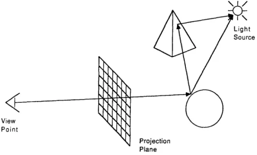
In a naive ray tracing algorithm, a ray is shot for each pixel from the view point into the 3D space as seen in Fig. 1. Each object is tested to find the first surface point hit by the ray. The color intensity at the intersection point is computed and returned as the value of the corresponding pixel. In order to compute the color intensity at the intersection point, the ray is then reflected from this surface point to determine whether the reflected ray hits a surface point or a light source. If the reflected ray ends at a light source, highlights or bright spots are seen on this surface. If the reflected ray hits another surface of an object, the color intensity at the new intersected point is also taken into account. This gives reflection of a surface on another. When the object is transparent, the ray is divided into two components and each ray is traced individually. 205

(2)

206

View

Point

VEYSi |~LER and Bt~LENT OZGf.3ff

Source

Projection

Plane

Fig. 1. Tracing of one ray.

As explained above, the color value at the intersection point gives the color value of the pixel associated with the intersecting ray. Therefore, having found the intersection point, the color at that point should be calculated according to a shading model. The following section includes a simple shading model which gives satisfactory results. Since this study is concerned mainly with the speedups obtained by different ray tracing algorithms, the given shading model is kept unchanged in all versions of the ray tracing system implementation discussed later.

2.1. The shading model

Initially the surface has ambient color which is a result of the uniform ambient light emitted by the surrounding objects. That is, a surface can still be visible even if it is not exposed directly to any light source. In this case, the surface is illuminated by the objects in its vicinity. Ambient color behaves similarly re- gardless of the viewing direction. We can express the intensity at a point on the surface of an object as

Color v = kaColora

where kd is the coefficient of reflection, and Colora is the ambient light intensity, kd takes values between 0 and 1; it is 1 for highly reflective surfaces. Unfortu- nately, ambient color alone does not give satisfactory results. Therefore, the effect of the light source(s) on the surface according to the orientation of the surface should also be considered in the computation of shading. That is, the diffuse reflections and the specular reflections add very much to the realism of the image. These computations use the reflection, normal, and other vectors as seen in Fig. 2. N is the unit vector normal to the point being shaded. L is the unit vector from the point to the light source. R is the unit vector in the reflection direction. The angle between R and

N is equal to the angle between V and N. V is the unit vector from the viewing point to the point on the surface.

Diffuse reflection computation is based on the Lam- bert cosine law, which states that the intensity of the reflected light depends on the cosine of the angle between the normal of the surface and the ray to the light [ 39 ]. The cosine of this angle is the dot product of two unit vectors in the light and normal vector directions.

Diffuse reflection is computed as

kdColort Color~ - - ( N . L )

d + d o

where Color~ is the intensity of the light source, d rep- resents the distance from a light source to the point being shaded and do is a constant to prevent denom- inator from approaching zero.

Highlights are seen from the view point when inci- dence light ray is at a certain angle and surface is shiny. The highlights (specular reflection ) can be modeled as

ksColort .

Cotor. = t K " L ) °

\

t

,,

(3)

Fast ray tracing 3D models

where n is a constant related to the surface optical property. It is zero if the surface is dull and very large if the surface is a perfect mirror, ks is a constant for specular reflection depending on the surface property. In order to simulate the reflection of surrounding objects on the point being shaded, a reflection ray is sent from this point and this ray is tested with the objects to find any intersection. If this ray hits any object, the color intensity at the intersected point contributes to our shading computation as follows:

Colorp = Colorp + k, Color,

where Colorp is the intensity computed previously for the point being shaded. Colorr is the intensity at the intersection point, kr is a constant that is related to the surface property; it is coefficient of reflection.

If the shaded object is transparent, the reflections from the objects behind it should also be considered. This reflection contributes to the shading computation

as

Color v = ( 1 - r)Color~ + rColorb.

Colort is the total intensity at the surface point after

summing the intensities of the ambient light, the diffuse reflection, and the specular reflection. Colorb is the in- tensity of the surface point behind the transparent object. r is a constant that is related to the transparency of the object. It is 0 if the object is opaque. In other words, the ray that hits a surface continues traveling through the transparent object until it intersects another object. The intensity at the intersection point is taken to contribute to the transparent object. This ray could also be refracted.

Shadows that give very strong depth cues to the image can be obtained while finding out the diffuse and specular reflections. The regions of a surface are in shadow if the light sources are blocked by any opaque or semitransparent object in the scene. This is found out by sending a ray from the point on the surface toward the light sources and testing for intersection of the ray with an object before the light source. If there is any intersection, both diffuse and specular reflections become zero.

3. SPEEDING UP THE ALGORITHM

As mentioned previously, the major drawback which prevents ray tracing from being attractive for interactive systems is its computational complexity due to many intersection tests between rays and objects. Whitted has estimated that up to 95% of the time is spent during these intersection tests [ 51 ]. They take too much time since all of the objects in the scene have to be tested to find the nearest intersection point with the ray, re- quiting intensive floating point operations. In order to reduce the processing time in the ray tracing algorithm, the computation for intersection tests should be de- creased. The use of coherence is the key point to speed up the ray tracing algorithm. The coherence that has

207

been exploited in many computer graphics algorithms to improve performance and image quality is the property that an environment or an image is locally constant and thus local information is utilized for efficient computations. The spatial, object, ray, and image coherence are different manifestations of coherence that have been widely used to enhance performance of the ray tracing significantly [ 3, l 1, 13, 27, 46 ]. Sev- eral considerations that might involve the use of coherence should be taken into account in order to reduce the computation time for the intersection tests: • An intersection test should be simple to compute.

That is, it should take a m i n i m u m number of computer cycles. The initial attempts to speed up the ray tracing were based on this approach. To make the intersection tests simple to compute, either intersection tests are made efficient or bounding volumes explained in the next section are used [ 20, 22, 35, 40, 44, 45 ].

• The number of objects to be tested for intersections should be as few as possible. Not all of the objects in the scene should be tested for intersection with the traced ray as in the naive ray tracing algorithm. Only objects that are highly possible for intersection should be tested. In other words, the objects on the ray's path should be considered for intersection tests. Several methods have been developed to achieve this. They are discussed in the next sections.

• Even if we could reduce the computation for a ray to a constant time, it is still necessary to process all of the pixels independently. Additionally, we may wish to shoot more than one ray for each pixel to increase the accuracy of the image. This means that the algorithm has another bottleneck due to the number of rays traveling in the scene. Thus, parallelism seems to be a logical solution for speeding up the ray tracing algorithm. Furthermore, ray tracing is highly amenable to parallelization on a multicomputer, since each primary ray is traced independently. Exploiting parallelism in ray tracing is discussed fur- ther in this section.

3.1. Bounding volumes

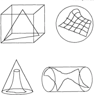
Some simple mathematically defined objects such as spheres, rectangular boxes, or cones can be tested for intersection with a minimal number of operations [14]. The complex objects are surrounded by these simple objects (bounding volumes), as in Fig. 3, and intersections are first tested with the bounding volumes instead of the complex objects. When the ray intersects the bounding volume of an object, tests are carried out for the complex object as well. Obviously, the advantage of using bounding volumes is to eliminate the intersection test with a complex object once its bounding volume is not intersected with the ray. Its disadvantage is the extra time spent in testing the bounding box if the object itself has a possible intersection. It should be noted that the bounding volumes are not mutually exclusive and, thus, a ray might be tested for an intersection with more than one object. This is an-

(4)

2O8 VEYSi i~;LER and

Fig. 3. Several types of bounding volumes.

other drawback of the bounding volumes, since an intersection test for a complex object may take excessive time. When this type of test is carried out more than once for a ray, it will be even worse.

When there is a large number of objects in the scene, even the tests for the bounding volumes can take an enormous amount of time. By forming a hierarchy of bounding volumes, a number of tests can be avoided once a bounding volume that surrounds some other bounding volumes is not hit by the ray. Several neighboring objects form one level of the hierarchy. The other drawback of this method is that these hierarchies are difficult to generate and manually generated ones can be poor. That is, they may not be helpful in speeding the intersection operation. Goldsmith has proposed methods for the evaluation of these hierarchies in ap- proximate number of intersection calculations required and for automatic generation of good hierarchies [ 15 ]. The bounding volumes used can be spheres, rectangular boxes, polyhedrons, parallel slabs, cones, or surfaces of revolution. The bounding volume chosen for each object in the scene can be different to enclose the object more tightly. This may be needed in order not to test more than one bounding volume for a ray.

3.2.

Spatial subdivision

A different approach to improve the efficiency of ray tracing is called space subdivision [11, 27]. The 3D space that contains the objects is subdivided into disjoint rectangular boxes so that each box contains a small number of objects. A ray travels through the 3D space by means of these boxes. A ray that enters a box on its way is tested for intersection with only those objects in the box. If there is more than one intersecting object, the nearest point is found and returned. If no object is hit, the ray moves to the next compartment (box) to find the nearest intersection there. This is re- peated until an intersection point is found or the ray leaves the largest box that contains all of the objects. It is necessary, in this case, to build an auxiliary data

BOLENT ()ZGO¢

structure to store the disjoint volumes with the objects attached to them [42, 43 ].

This preprocessing will require a considerable amount of time and memory as a price for the speedup in the algorithm. It is, however, worth using the space subdivision particularly when the scene contains many objects, since this data structure is constructed only once at the beginning and is used during the ray tracing algorithm. The number of rays traced depends both on the resolution of the generated image and the number of objects in the scene. The auxiliary data structure helps to minimize the time complexity of the algorithm by considering only those objects on the ray's way.

There are several techniques that utilize space coherence. They basically differ in the auxiliary data structures used in the subdivision process, and the manner used to pass from one volume to another.

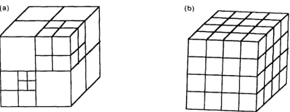
In some ray tracing schemes that utilize the spatial coherence, the space subdivision process is based on the octree spatial representation. An octree is a hierarchical data structure organized such that each node can point to one parent node and 8 leaf nodes. Fig. 4 shows this type of subdivision of the space. In the spatial subdivision ray tracing algorithm, each node of the octree corresponds to a region of the 3D space [12, 13, 15 ]. The octree building starts by finding a box that includes all of the objects in the scene. A given box is subdivided into 8 equally sized boxes according to a subdivision criterion. These boxes are disjoint and do not overlap as the bounding volumes might do. Each of the generated boxes are examined to find which objects of the parent node are included by each child node. The child nodes are subdivided if the subdivision criterion is satisfied. This is carried out recursively for each generated box.

The subdivision criteria may be based on the number of objects in the box, the size of the box, and the density ratio of total volume that is enclosed by all objects in the scene to the volume of the box. When the criterion for the number of objects in a given box is very large, each object in the scene is tested for intersection for all rays as in the naive algorithm. No speedup will be achieved; on the contrary, the time and the memory will be wasted for the octree data structure. On the other hand, if the number of objects is one for the criterion, there will be many boxes in the structure and the overhead for traveling through the 3D space may increase.

Kaplan used a data structure which he calls the BSP (Binary Space Partitioning) tree to decompose the 3D space into rectangular regions dynamically [ 27 ]. BSP is very similar to octree structure in that it also divides the space adaptively. The information is stored as a binary tree (a tree where each nonterminal node can have exactly two child nodes) whose nonleaf nodes are called slicing nodes, and whose leaf nodes are called box nodes and termination nodes. Each slicing node contains the identification of a slicing plane, which divides all of space into two infinite subspaces. The slicing planes are always aligned with two of the Carte- sian coordinate axes of the space that contains the oh-

(5)

(a)

Fast ray tracing 3D models (b)

L ,Z / ,Z

209

I

Fig. 4. (a) Adaptive subdivision, (b) Subdivision of space into equally sized cubes.

jects. The child nodes of a slicing node can be either other, termination nodes, slicing nodes or box nodes. A termination node denotes a subspace which is out of the 3D space that does not contain any objects. A box node, on the other hand, is described by the slicing nodes that are traversed to reach it. They denote a subspace containing at least one object. BSP actually encodes the octree in the form of a binary space partitioning tree and it is traversed to find the node containing a given point.

The other spatial subdivision technique for ray tracing is based on the decomposition of the 3D space into equally sized cubes [11]. Fig. 4 contains a scene decomposed into equally sized volumes. The size of the cubes determines the number of objects in each cube. Therefore, an optimal cube size must be considered such that the overhead for moving through the boxes should not exceed the time gained in testing intersections.

Fujimoto proposed a scheme that imposes an auxiliary structure called SEADS (Spatially Enumerated Auxiliary Data Structure ) on objects in the scene [ 11 ]. This structure uses a high level of object coherence. He also developed a traversing tool that fits in well with SEADS to take advantage of the coherence in a very efficient way based on incremental integer logic. This method, called 3DDDA (3D Digital Differential Analyzer), is a 3D form of the 2D digital-differential analyzer algorithm commonly used for line drawing in raster graphics system. The major advantage of this scheme is related to the manner to travel through 3D space containing the objects. 3DDDA does not require floating-point multiplications or divisions in order to pass from one subspace (voxel) to the next while look- ing for intersections, once a preprocessing for the ray has been performed. Fujimoto states that an order of magnitude improvement in ray tracking speed over the octree methods has been achieved. It is also possible to improve the performance of octree traversal by uti- lizing the 3DDDA method to traverse horizontally in the octree, but vertical level changes must be traversed as usual.

3.3.

A hybrid technique

Recently, Glassner has presented techniques for ray tracing of animated scenes efficiently [ 14 ]. In his technique, he renders static 4D objects in spacetime instead

of rendering dynamically moving 3D objects in space. He uses 4D analogues familiar to 3D ray-tracing techniques. Additionally, he performs a hybrid adaptive space subdivision and bounding volume technique for

generating good, nonoverlapping hierarchies of

bounding volumes. The quality of the hierarchy and its nonoverlapping property is an advantage over the previous algorithms, because it reduces the number of ray-object intersections that must be computed.

The procedure to create such a hierarchy starts by finding a box that encloses all of the objects in the scene, including light sources and the view point. The algorithm then subdivides the space adaptively as in the octree method. The subdivision that is based on a given criterion is performed for each box recursively. The recursion is terminated when no boxes need to be subdivided.

As returning from the recursive calls made by the space subdivision process, the bounding volume hierarchy is constructed. Each box is examined, and a bounding volume is defined that encloses all the objects included within that box. The defined bounding volume must not intersect any other box. That is, it is clipped by the space subdivision box.

At the end of this process, a tree of bounding volumes that has both the nonoverlapping hierarchy of the space subdivision technique and the tight bounds of the bounding volume technique is constructed. Thus, the new hierarchy has the advantages of both approaches while avoiding their drawbacks.

3.4.

Parallel ray tracing

The recent development in VLSI technology has made it feasible to design and implement special purpose hardware for the ray tracing algorithm [40]. In spite of the gain obtained in this way, these special purpose architectures have several disadvantages. Pri- marily, there are still studies to improve the algorithm itself. Researchers should thus work on general purpose machines in order not to be restricted by the hardware. Secondly, special purpose hardware is expensive and often restricts the applications that require other computer graphics algorithms.

Another approach that exploits speedup through the inherent parallelism in ray tracing investigates the algorithm on a general purpose parallel architecture independent of the hardware configuration [7, 10, 17,

(6)

210 VEYSi {~LER and BOLENT OZGt3(~ 18, 28-30, 36 ]. In the next subsections, parallelization

of the ray tracing algorithm on a multicomputer is investigated. The effective parallelization of the ray tracing algorithm on a multicomputer requires the partitioning and mapping of the ray tracing computations and the object space data. This partitioning and mapping should be performed in a manner that results in low interprocessor communication overhead and low processor idle time. Two basic schemes are presented for parallelization. In the first scheme, discussed in Section 3.4.1., only ray tracing computations are partitioned among the processors. In the scheme discussed in Section 3.4.2., both ray tracing computations and object space data are partitioned among the processors.

3.4.1. Image space subdivision. In this scheme, the overall pixel domain of the image space to be generated is decomposed into subdomains. Then, each pixel sub- domain is assigned to and computed by a different processor of the multicomputer. However, each processor should keep a copy of the entire information about the objects in the scene in order to trace the rays associated with the pixels assigned to itself. Hence, an identical copy of the data structure representing the overall object space is duplicated in the local memory of each processor. This scheme requires no interprocessor communication since the computations associated with each pixel is independent of each other.

Assignment ofpixels to processors can be either static or dynamic. In the static scheme, the pixel subdomains are assigned to the processors before the execution of the algorithm. However, even decomposition and assignment of the overall pixel domain does not guar- antee even workload for the processors. The amount of computation associated with individual pixel may be quite different depending on the location of the pixels and the configuration of the objects in the scene. Furthermore, computational complexity associated with a pixel cannot be predetermined.

The simplest way of static assignment is tiled de-

composition where the image space is partitioned evenly into contiguous blocks of pixels and each pixel

block is then assigned to a processor. Fig. 5(a) illustrates tiled assignment for 16 × 16 image space and 8 processors. Most probably, each block will require a different amount of computation, which is the source of load imbalance among processors. For example, rays generated at some processors might leave the scene very soon without intersecting any object. These processors will complete their jobs earlier than others re- suiting in poor processor utilization. Load imbalance

problem is solved to an extent by applying scattered

subdivision which is based on the assumption that adjacent pixels require almost the same amount of computation. Scattered decomposition scheme is achieved by imposing a periodic processor mesh template over the image pixels starting from the top left corner and proceeding left to right and, top to bottom. Fig. 5(b) illustrates the scattered decomposition for 16 × 16 image space and 8 processors. In this scheme, adjacent pixels are assigned to different processors. Hence, this scheme achieves better load balance that distributes the workload to processors more evenly. In this scheme,

each processor is responsible for pixels which are scat-

tered across the entire image. In the worst case, scat- tered decomposition will behave as tiled decomposition that has led to load imbalance. However, such cases are extremely unlikely to be encountered. Therefore,

scattered decomposition usually performs better than

tiled decomposition.

In the dynamic scheme, tiled decomposition is ap-

plied in partitioning the image space assuming very large number of processors. The contiguous pixel blocks are then dynamically assigned to processors in an "on demand" policy. The pool of pixel blocks is resident in a special processor called the scheduler. The scheduler is responsible for the assignment of pixel blocks to the demanding processors. The size of pixel block is the number of pixels assigned to a processor on a single request. Each such request requires an extra communication between the requesting processor and the scheduler. Hence, the pixel block size determines the granularity of the distributed computations on the multicomputer. Large pixel block sizes increase the

o l o o i o o { o o o i 1 1 i i i i 1 1

oio olo o,o' o o ,!ill 1 1 i 1

o l o o o o l o o o { I i 1 ! 1 1,1 1 1

oio 0 0 0,0,0 011i1,1 lii

11 2, 222i22 31 33333{

{

2 2 2 2 1 2 2 2 3 3 3 3 3 3 3

2 2 2 2 2 2 2 3 i 3 3 3 3 3 3

2 2 2 2 2 2 2 3 3 3 3 3 3 3

4 4 4 4 1 4 4 4 5 5 5 5 5 5 5 4 4 4 4 1 4 4 4 5 5 5 5 5 5 5 4 4 4 4 1 4 4 4 5 5 5 5 5 5 5 4 4 4 4 4 ! 4 ! 4 4 5 ] 5 5 5 5 5 5

565o551557! i 7777

_{6 6 6 6 6 1 ~ 1 6 5 7 7 7 7 7 7 7}

5 6 6 6 5

6 5 7 7 7 7 7 7 7

5 6 5 6 6 i 6 6 6 7 7 7 7 1 7 7 7

!i

o 4 b 1 4 3 0 5 4 3 5 4 5 0 5 4 5 0 5 4 7 0 7 4 7 0 7 4 1 2 ; 3

011 2 3 011i21310 I',2 3

5 617 4 5 6 7 4 516{ 7 4 5 ! 6 7 1 2 i 3 0 1 2 3 0 1 1 2 1 3 0 1 ~ 2 '3 5 5 7 7 4 5 6 7 4 5 5 j 7 4 5 { 5 7 1 2 i 3 0 1 2 3 0 1 2 ! 3 0 l l 2 3 5 5i 7; 4 5 6 7 4 5 5 7 4 5 6 7 1 2 ~ 3 0 1 2 3 0 1 2 ] 3 0 1 ] 2 3 5 5 i 7, 4 5 6 7 4 5 5 [ 7 4 5 i 5 7 1 2 : 3 0 1 2 3 0 1 2 3 0 1 i 2 3 5 6 , 7 4 5 5 ' 7 4 5 i 5 { 7 4 5 i 6 7 1 2 i 3 0 1 2 3 0 1 2 ] 3 0 1 i 2 3 1 2 3 1 2 3 o 1L~!a o 1 1 2 3 5 6 [ 7 5 6 7 4 5 5{7 4 5 5 7 1 2 1 3 1 2 3 0 1 1 3 0 1 2 3 5 6 i 7 5 6 7 4 5 1 7 4 5 6 (a) (b)

(7)

Fast ray tracing 3D models 211 performance of the algorithm by decreasing the number

of the c o m m u n i c a t i o n s between the scheduler and the processors. On the other hand, large pixel block size degrades the performance by introducing load imbalance between processors. For an appropriate granularity, the performance is excellent in terms of load imbalance, since processors are assigned to the computations of a new pixel block as soon as they b e c o m e idle. This scheme approaches the static tiled decom- position scheme as the n u m b e r of pixel blocks are reduced to the n u m b e r of processors. The overhead im- posed by this scheme is the c o m m u n i c a t i o n between scheduler and the processois.

The image space subdivision achieves almost a linear speedup. No c o m m u n i c a t i o n is needed between processors. The only overhead is the c o m m u n i c a t i o n between the scheduler and the processors of the multicomputer. On the other hand, each processor should have access to the whole scene description, since ray- object intersection tests may be carried out with any object in the scene. This is a great disadvantage of the image subdivision scheme. In more realistic scene descriptions, a huge a m o u n t of storage is needed to hold the object definitions and other related information. Therefore, processors cannot store the entire information about the objects in the scene.

3.4.2. Object space subdivision. Through some means, the object space is to be subdivided and stored in the local memories of processors. The subdivision of the object space necessitates interprocessor communication. We can classify the existing object space algorithms into two: some are based on the m o v e m e n t of objects between processors, and others are based on the m o v e m e n t of rays between processors.

In the first class, the read-only database is distributed to local memories of different processors. Each processor generates a set of rays associated with the pixels assigned to itself. W h e n a processor needs a part o f the scene description for intersection tests that is not available in its local memory, a request is sent to the processor that contains this part o f the database. The related information is copied or m o v e d to the requesting processor's memory. The local memories behave as a

cache and contain the object descriptions according to

L R U replacement policy. This class of algorithms suf- fers from communication volume overhead that results from migration of objects between the processors.

T w o approaches exist in the second class. In the first approach, the 3D space containing the objects is subdivided into several disjoint volumes. The computation related to the objects in a v o l u m e is carried out by a specific processor. The ray that travels through 3D space to find an intersection passes from one processor to another via messages. Each processor contains the information about the v o l u m e assigned to itself.

The other approach in object-based subdivision constructs a hierarchy of bounding volumes. The objects in the same bounding v o l u m e are stored in one processor. A processor shoots a primary ray and follows it through the hierarchy down to the leaf nodes of this hierarchy that are pointers to the processor in which

the appropriate part of the database is stored. If this traversal ends at a pointer to itself, the necessary calculations are performed for the pixel associated with the ray, otherwise the ray is sent to the concerned processor. Each processor thus controls a block of pixels, the hierarchy, and a portion of the database.

In object-based type of algorithms, the load imbalance is the major problem to deal with, since some processors may contain objects that are more likely to be intersected than others. This may even result in the deadlock of the system due to a large n u m b e r of messages traveling around,

4. SOFI'WARE OVERVIEW

A fast ray tracing system is designed and implemented in the C programming language on S U N ' Workstations running under U N I X 2 operating system. The system has three major parts:

• Model a 3D scene with objects provided by the system.

• Process the defined scene to obtain a realistic image that consists of R G B values.

• Display the generated image.

The system can be used mainly to create scenes containing 3D objects and then find out the effect of light sources and the objects on each other. Each part is to be explained in detail in the following sections.

4.1. Interactive 3 D modeler

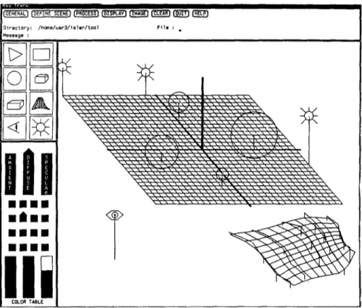
This is used in the first step of generating a realistic image. To provide the user with a friendly environment, SunView 3 has been used for creating panels, menus, buttons, etc. [471 . More information about multi-window e n v i r o n m e n t can be found in ref. 38. The user gives the description of a scene using mouse, menus, etc. This tool projects the 3D world onto the 2D screen to provide user with an easy user interface when entering 3D points as shown in Fig. 6.

Using this tool, the scene description mainly involves selecting one of the object types and specifying the size and other parameters related to the selected object type by the mouse, panel, and other windowing system ele- ments. The user is provided with five primitive types of objects to model the scene. They are sphere, triangle, rectangle, box, and superquadric. In addition to the definition of objects to be included in the scene, the user can give values to a n u m b e r of parameters. They are point light sources, viewpoint, origin of the scene, screen size, viewport, orientation of the viewpoint, level of reflection, etc. The processing is carried out with these parameters if they are specified by the user. Oth- erwise, they are assigned default values.

The object definition starts by selecting the corresponding icon and inputting the necessary size and position information about the selected object. The ' SUN Workstation is a registered trademark of Sun Mi- crosystems, Inc.

2 UNIX is a registered trademark of AT&T Bell Labora- tories.

(8)

212 VEYSi I~LER and BIDLENT (~ZGf3~ l i r i , n i ~ l ~ Directory: / h o ~ a / u s r 3 / I s l o r / t o o l F i l e : • Messsge : , , , , , x \ ^ x x x \ x \ \ ~ x ~ x \ ~ \ x \ l \ x ~ x / x \ \ x \ \ \ \ \ i , \ x ~ x x - . x x ~ x ~ x x ~ \ \ ~ \ x \ i x \ \

Jill

u m m m

m l m m

m m m m

\ . . . . 1 , , ~ . . . xx\ ~x ~ x~ x^x xx -. x~ xx xxx xx x\ xx xxx X \\\ \x~ \ " . / , x x~ x x xl ' . n ~ xx \\ x x\ \\ \\ X , \ , \ ~ x x \ x x x x x x x ~ x \ \ ' ~ \ \ \ t x x x x x x x \ \ \ x x x x x \ \ \ \ \ \x x x x x xx x x ~ x \ xx ~ \ x x \x \ xx x x x \ \ \ % N ' % N N % N \ N \ N x x x x x ~ x \ x x x x x ~ x ~ x ~ @ x x x % x x x ~ x x \ x @ x X x k x ~ \ ~ x ~ N ~ N N N \ x xx x x x~ xn x x xx x x x xx n x \~ x \ n xx x \ x

Fig. 6. Interactive 3D modeler.

size and position information for the objects is specified by 3D points. Three coordinate axes and y - z plane as a reference is drawn on the canvas where 3D points are given for the objects, light sources, a n d view point. That is, 3D space is projected on the 2D screen to be able to get the 3D inputs. A point in 3D space is entered by first pointing at x - z plane a n d pressing a mouse button at that point, then dragging either up or down to enter the y-coordinate. In other words, first x, z- components are given, next the y c o m p o n e n t of the point is denoted by releasing the mouse button. The y - c o m p o n e n t is the difference between the heights of releasing point and pressing point.

Every object should refer to a n u m b e r called "surface n u m b e r " that must be defined to denote the material properties of the object referring to it. Surface definition gives the material property of the object with its color and consists of the following information:

• a m b i e n t color, • diffuse color, • specular color, • surface coefficient, • reflection, and • transparency.

The color values are given using the panel at the bottom. There are 16 predefined colors displayed in small squares. The user can select one of these and load it into ambient, diffuse, or specular boxes that are above the color squares. The color of a selected square can be changed by sliding the red, green, or blue compo-

nents. The background color is taken from the last square in the panel.

After completing the description of the scene, the system converts it into the format that is accepted by the ray tracing module and writes the textual description on a text file. Therefore, this interactive tool is nothing but a shell that generates the description on a text file as an output. The textual description of a scene is useful in the sense that the ray tracer can be portable to any computer system.

4.1.1. B-spline surfaces. The other advantage of the

interactive tool is that the user can generate free-form surfaces other than five primitive object types. Free- form surfaces can be created and placed into an appropriate location in the scene. B-Spline method is used by the system to find out the surface to be included in the scene description. The surface generated is then triangulized and written in the known format on the output file as a collection of triangle primitives.

Since objects with complex shapes occur frequently in our 3D world, special techniques to model them properly are needed [ 37 ]. Although these objects can be approximated with arbitrarily fine precision as plane-faced polyhedra, such representations are bulky and intractable. For example, a polyhedral approxi- mation of a hat might contain 1000 faces a n d would be diffcult to generate and to modify. We need a more direct representation of shapes, easy both to the computer and to the person trying to manipulate the shapes. Brzier and B-spline are the two methods frequently used to generate curves and surfaces of 3D. They are

(9)

I

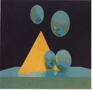
Fig. 7. Four spheres and a triangle. _{Fig. 10. Twenty four spheres.}

Fig. 8. Fifty spheres.

Fig. 11. Sphere above chessboard.

Fig. 9. Two hundred spheres. Fig. 12. Shield and a sphere.

(10)

214 VEYSi I~;LER and B(3LENT OZGt3~7

similar to each other in that a set of blending functions is used to combine the effects of the control points. The key difference lies in the formulation of the blending functions [4, 21, 37].

4.2. Processing: Ray tracer

This part accepts a textual scene description as input and generates an image containing several optical effects for the sake of realism using the ray tracing algorithm.

The shading model used by the system is similar to the one given in section 2. This part of the system has three different versions. The first version of the system is based on the naive ray tracing algorithm. That is, all objects in the scene are tested to find the first intersection with a traced ray. As it is very obvious, the time spent increases with the number of objects in the scene.

In the second version of the ray tracing system, the intersection tests are not carried out with all objects in the scene but the spatial coherence technique is used to perform intersection tests only for the objects that are on the path of the ray. Therefore, the space containing the objects is subdivided using the octree representation. The second version of the program is ca- pable of generating the images much faster than the first version that does not utilize the space coherence. The last version is the parallel ray tracing algorithm and presented in the next subsection.

4.2.1. Parallel ray tracer. The parallel ray tracer is

implemented in the C programming language on iPSC4/2 hypercube [24]. The ray tracer consists of two parts: one on hypercube and the other on the SUN workstation. The hypercube host and the SUN workstations are connected to each other via the ethernet. While the pixel values are computed on the hypercube, a color SUN workstation receives them through the UNIX internetworking sockets interface and displays them immediately.

The server on the hypercube has two kinds of processes that run on the nodes and host. The node processes are responsible for the computation of the pixel values assigned to them. The assignment of pixels can be either static or dynamic. All nodes have the whole scene description at their 4MB local memory. The only communication is between the host and the node processors.

Scattered decomposition of the image space is performed for static assignment of workload as in Fig. 5. After a predetermined number of pixels is computed by a node, the resultant pixel values are sent to the host.

In the dynamic scheme, the pixels of the image space are allocated to the nodes on demand. The host serves as both scheduler to distribute the pixeis and collector of the computed pixel values. Two types of communications are defined for transferring the resultant pixel values and specifying the pixels to be computed.

The node processes start as soon as they receive the 4 iPSC is a registered trademark of Intel Corp.

second type of message that contains the coordinates of several consecutive pixeis. When a node process fin- ishes with its computations, it sends the result to the host and makes a request for another pixel block. On the other hand, host waits for the results from the nodes and assigns another consecutive pixel block to the requesting node. The node processes exit when they receive an invalid coordinate for pixels indicating that no more pixels remained on the host to be distributed to the nodes. The ray tracer uses the spatial coherence to avoid many intersection tests [ 13 ]. The 3D space is subdivided into disjoint volumes in octree fashion. Every node owns this auxiliary data structure and only the objects on the ray's path are tested for intersection. Although the load balance is ensured by the algorithm and the speedup is linear, its drawback is in the duplication of the database in every node.

4.3. Displaying the image

We compute a triple (RGB) for each pixel of the image after tracing a ray. When we compute RGB values in shading routine, we assume a linear intensity response. That is, the pixel of a value of 127, 127, 127 has the half intensity of a pixel value 255, 255, 255. However, the response of typical video color monitors and of the human visual system is nonlinear. Thus, displaying of images in a linear format results in effective intensity quantization at a much lower resolution than the available 256 resolution per color. That is, the true colors will not be perceived by the human eye, because of the nonlinearity in the monitor. Therefore, it is necessary to correct the computed values so that the generated picture appears more realistic to a human observer.

A function called gamma correction is used for this purpose [19]. It is an exponential function of the form:

lookupvalue = intensity t'°/gamma.

G a m m a represents the nonlinearity of the monitor. Generally monitors have a gamma value that is in the range 2.0 to 3.0. If gamma is equal to 1, the device is a linear one. An incorrect value results in incorrect image contrast and chromaticity shifts. If the gamma is too small, the contrast is increased and the colors approach to the primaries.

The RGB values should be corrected by the above function before the image is displayed or stored to a file.

4.4. Examples and timing results

In this section, several images generated by our system are presented in Figs. 7-12. We also compare the time spent in the first, second and third version (dynamic scheme) of the algorithms for some images. Ta- ble 1 contains the clock timings for rendering three images given in Figs. 7-9. Actually, there may be several other influences on the rendering time other than the complexity of the algorithm. These are the programming style, code optimization, processor speed,

(11)

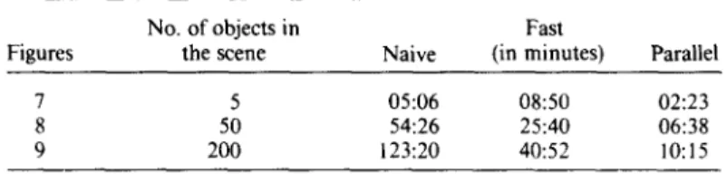
Fast ray tracing 3D models Table 1. Timing results of Figs. 6, 7, and 8.

No. of objects in Fast

Figures the scene Naive (in minutes) Parallel

7 5 05:06 08:50 02:23

8 50 54:26 25:40 06:38

9 200 123:20 40:52 10:15

215

n u m b e r o f objects in the scene increases, the ratio of the naive technique to the fast one gets larger and larger. This is due to the fact that a great a m o u n t of time is wasted for the intersection calculations in the naive ray tracing system. The ratio approaches one for the scenes containing few n u m b e r of objects [25].

In higher speed models, we note that the timings are dependent on the criteria used to subdivide the space. For example, when the space is divided into very small boxes that contain only one object, the overhead for traveling through the boxes may approach to the time saved for intersection tests. That is, the ray may frequently pass through m a n y empty volumes wasting a considerable a m o u n t of time. Table 2 shows timings for the image in Figure 10 generated using the octree auxiliary data structure for three different ter- minating criteria values.

In the parallel version, we observe that speedup is almost linear and load balance is satisfied with the al- location of pixels to processors on demand. Granularity is a variable that must be adjusted to an optimal value both to maintain the load balance and to avoid excessive communication. Table 1 includes the clock timings for three images given in Figures 7 - 9 generated by the parallel ray tracer using 4 processors of hypercube.

5. CONCLUSIONS

Computer-generated images that appear realistic to a human observer have been one of the most important goals in c o m p u t e r graphics. The ray tracing algorithm, in this respect, is the most popular m e t h o d for realistic image synthesis. It is in the class of image generation algorithms, called global shading, that provide the most realistic images by considering the optical effects such as shadowing and reflection from the surfaces in the environment. However, it requires a tremendous a m o u n t of time to generate an image. Several methods have been developed to o v e r c o m e the time problem [7, 10-14, 27, 34, 35]. In this article, we investigated these methods and used two of them, namely space subdivision and parallelism, in the implementation of the ray tracing system. The space subdivision m e t h o d saves a considerable a m o u n t of time when the scene

Table 2. Timing results of Fig. 9.

No. of objects Time

in boxes (in minutes)

2 22:21

5 18:07

10 29:45

is complex. But the speedup achieved is still not enough when m a n y images are to be generated. The parallel version o f the space subdivision method may be the best solution for the time problem. As for the first conclusion, the parallelism is essential for the interactive realistic image generation.

Finally, we should also take into account the texture mapping that is used to cover over a surface with texture [5], in order to provide more detailed images. Texture mapping is basically the method of wallpa- pering the polygons in the scene. O n e of the future directions in realistic image generation is to develop methods for ray tracing texture mapped surfaces in a reasonable a m o u n t of time.

REFERENCES

1. J. Amanatides, Ray tracing with cones. ACM Computer

Graphics 18(3), 129-135 (July 1984).

2. J. Amanatides, Realism in computer graphics: A survey.

IEEE CG&A 44-56, (January 1987).

3. J. Arvo and D. Kirk, Fast ray tracing by ray classification.

ACM Computer Graphics 21(4), 55-64 (July 1987).

4, B.A. Barsky, A description and evaluation of various 3D models. IEEE CG&A (January 1984).

5. J. F. Blinn and M. E. Newell, Texture and reflection in computer generated images. Communications ~?[the ACM 19(10), 542-547 (October 1976).

6. C. Bouville, R. Brusq, J. L. Dubois, and I. Marchal, Gen- erating high quality pictures by ray tracing. Computer

Graphics Forum 4, 87-99 (1985).

7. J.G. Cleary, B. M. Wyvill, G. M. Birtwistle, and R. Vatti, Multiprocessor ray tracing. Computer Graphics Forum 5, 3-12 (1986).

8. M. F. Cohen and D. P. Greenberg, A radiosity solution for complex environments. A C M Computer Graphites

(Proc. S1GGIL4PH) 19(3), 31-40 (July 1985 ).

9. R. L. Cook, T. Porter, and L. Carpenter, Distributed ray tracing. A (~1 Computer Graphics 18 (3), 129-135 (July

1984).

10. M. Dipp6 and J. Swensen, An adaptive subdivision algorithm and parallel architecture for realistic image syn- thesis. ACM Computer Graphics 18(3 ), 149-158 (July

1984).

11. A. Fujimoto, T. Tanaka, and K. lwata, ARTS: accelerated ray-tracing system. IEEE CG&4, 16-26 (April 1985 ). 12. W. Geoff, Space division for ray tracing in CSG. 1EEE

CG&A. 28-34 (April 1986).

13. A. S. Glassner, Space subdivision for fast ray tracing. 1EEE

CG&A, 15-22 (October 1984).

14. A.S. Glassner, Spacetime ray tracing for animation. IEEE

CG&A, 60-70 (March 1988).

15. J. Goldsmith and J. Salmon, Automatic creation of object hierarchies for ray tracing. 1EEE CG&4, 14-20 (May

1987).

16. C. M. Goral, K. E. Torrance, D. P. Greenberg, and B. Battaile, Modeling the interaction of light between diffuse surfaces. A C M Computer Graphics, 18(3), 213-222 (1984).

17. S. A. Green, D. J. Paddon, and E. Lewis, A parallel algorithm and tree-based computer architecture for ray-

(12)

216 VEYSi |~LER and BOLENT C)ZGO~ traced computer graphics. International Conference,

University of Leeds, UK (January 12-15, 1988). 18. S. A. Green and D. J. Paddon, Exploiting coherence for

multiprocessor ray tracing. IEEE CG&A, 12-26 (No-

vember 1989).

19. R. Hall, Color reproduction and illumination models. In

Techniques for Computer Graphk~, Springer-Verlag, New

York, 195-238 (1987).

20. P. Hanrahan, Using caching and breadth-first search to

speed up. Proc. Graphics and Vision Interface '86, Ca-

nadian Information Society, Toronto, 56-61 (1986).

21. D. Hearn and M. P. Baker, Computer Graphics', Prentice-

Hall, Inc., Englewood Cliffs, NJ ( 1986 ).

22. P. S. Heckbert and P. Hanrahan, Beam tracing polygonal

objects. ACM Computer Graphics 18(3), 119-127 (July

1984).

23. D. S. lmmel, M. F. Cohen, and D. P. Greenberg, A ra-

diosity method for non-diffuse environments. ACM

Computer Graphics (Proc. SIGGRAPH). 133-142

(1986).

24. lntel Corporation, iPSC/2 Programmer's Reference

Manual, Santa Clara, CA (1989).

25. V. l~ler and B. Ozg0q, Ray tracing geometrical models.

Proc. 4th hit. Symp. Comp. Info. Sci., Ce~me, Turkey,

vol. 1,493-505 (October 1989).

26. J. T. Kajiya and B. P. V. Herzen, Ray tracing volume

densities. ACM Computer Graphics 18 (3), 165-174 (July

1984).

27. M. R. Kaplan, The use of spatial coherence in ray tracing.

Techniques for Computer Graphics', Springer-Verlag, New

York, 173-193 (1987).

28. H. Kobayashi and T. Nakamura, Parallel processing of

an object space for image synthesis using ray tracing. The

Visual Computer, No. 3, 13-22 (1987).

29. H. Kobayashi, S. Nishimura, H. Kubota, T. Nakamura, and Y. Shigei, Load balancing strategies for a parallel ray-

tracing system based on constant subdivision. The Visual

Computer, No. 4, 197-209 (1988).

30. D. J. Plunkett and M. J. Bailey, The vectorization of a

ray-tracing algorithm for improved execution speed. 1EEE

CG&A. 52-60 (August 1985).

31. R. Kuchkuda, An introduction to ray tracing. In Theo-

retical Foundations of Computer Graphics and CAD,

R. A. Earnshaw (ed.), NATO ASI Series, vol. F40, Springer-Verlag, Berlin, Heidelberg, 1039-1060 (1988). 32. W. Leister, T. Maus, H. MOiler, B. Neidecker, A. Schmitt, and S. Achim, Occursus cum novo: Computer animation

by raytracing in a network. Technical Report. Universit~it

Karlsruhe, Fakult~it FOr Informatik (November 1987 ). 33. G. Levner, P. Tassinari, and D. Marini, In A simple, gen-

eral method for ray tracing bicubic surfaces. Theoretical

Foundations of Computer Graphics and CAD, R. A.

Earnshaw (ed.), NATO ASI Series, vol. F40, Springer- Verlag, Berlin, Heidelberg, 805-820 (1988).

34. H. MOiler, Ray tracing complex scenes by grids. Technical

Report, Universi~t Karlsruhe, Fakult~it Fiir Informatik

(December 1985).

35. H. M011er and H. Hagen, Trading speed against space in

ray tracing free form surfaces. Technical Report, Univ-

ersit~it Karlsruhe, Fakult~it Fiir lnformatik ( May 1986 ). 36. K. Nemoto and T. Omachi, An adaptive subdivision by

sliding boundary surfaces. Proc. Graphics and Vision In-

terface '86, Canadian Information Society, Toronto, 43-

48 (1986).

37. W. Newman and R. Sproull, Principles" of Interactive

Computer Graphics, 2 ed., McGraw-Hill, New York

(1981).

38. B. ()zg0~, Thoughts on user interface design for multi

window environments. Proc. 2nd Int. Syrup. Comput.

Info. Sci., lstanbul, Turkey, 477-488 (1987).

39. B. T. Phong, Illumination for computer generated pic-

tures. Communication oftheACM 18(6), 311-317 (June

1975).

40. R. Pulleyblank and J. Kapenga, The feasibility ofa VLSI

chip for ray tracing bicubic patches. IEEE CG&A, 33-

44 (March 1987).

41. S. Sahni and S. Ranka, Hypercube Algorithms for Image

Processing and Pattern Recognition, Springer-Verlag, New

York (1990).

42. H. Samet and R. E. Webber, Hierarchical data structures and algorithms for computer graphics, Part I: Funda-

mentals. IEEE CG&A, 48-68 (May 1988 ).

43. H. Samet and R. E. Webber, Hierarchical data structures and algorithms for computer graphics, Part II: Applica-

tions. 1EEE CG&A, 59-75 (July 1988).

44. A. Schmitt, H. MOiler, and W. Leister, In Ray tracing

algorithms--Theory and practice. Theoretical foundations

of Computer Graphics and CAD. R. A. Earnshaw (ed.),

NATO ASI Series, vol. F40, Springer-Verlag, Berlin, Hei- delberg 997-1030 (1988).

45. T. W. Sederberg and D. C. Anderson, Ray tracing ofstei-

ner patches. ACM Computer Graphics 18(3), 159-164

(July 1984).

46. M. Shinga, et al., Principles and applications of pencil

tracing. ACM Computer Graphics 21(4), 45-54 (July

1987).

47. Sun Microsystems, Sun View Programmer's Guide,

Mountain View, CA (1986).

48. Sun Microsystems, UNIX Interface Reference Manual,

Mountain View, CA (1986).

49. J. R. Wallace, K. A. Elmquist, and E. A. Haines, A ray

tracing algorithm for progressive radiosity. ACM Com-

puter Graphics 23(3 ), 315-324 (July 1989).

50. G. Ward, et al., A ray tracing solution for diffuse inter-

reflection. A CM Computer Graphics 22 (4), 85-92 ( Au-

gust 1988).

51. T. Whitted, An improved illumination model for shaded

display. Communications of the ACM 23, 343-349 (June