Perceptual watersheds for cell segmentation in fluorescence microscopy images

PERCEPTUAL WATERSHEDS FOR CELL

SEGMENTATION IN FLUORESCENCE

MICROSCOPY IMAGES

a thesis

submitted to the department of computer engineering

and the graduate school of engineering and science

of bilkent university

in partial fulfillment of the requirements

for the degree of

master of science

By

Salim Arslan

August, 2012

I certify that I have read this thesis and that in my opinion it is fully adequate, in scope and in quality, as a thesis for the degree of Master of Science.

Assist. Prof. Dr. C¸ i˘gdem G¨und¨uz Demir(Advisor)

I certify that I have read this thesis and that in my opinion it is fully adequate, in scope and in quality, as a thesis for the degree of Master of Science.

Assoc. Prof. Dr. Reng¨ul C¸ etin Atalay

I certify that I have read this thesis and that in my opinion it is fully adequate, in scope and in quality, as a thesis for the degree of Master of Science.

Assist. Prof. Dr. Pınar Duygulu S¸ahin

Approved for the Graduate School of Engineering and Science:

Prof. Dr. Levent Onural Director of the Graduate School

ABSTRACT

PERCEPTUAL WATERSHEDS FOR CELL

SEGMENTATION IN FLUORESCENCE MICROSCOPY

IMAGES

Salim Arslan

M.S. in Computer Engineering

Supervisor: Assist. Prof. Dr. C¸ i˘gdem G¨und¨uz Demir August, 2012

High content screening aims to analyze complex biological systems and collect quantitative data via automated microscopy imaging to improve the quality of molecular cellular biology research in means of speed and accuracy. More rapid and accurate high-throughput screening becomes possible with advances in au-tomated microscopy image analysis, for which cell segmentation commonly con-stitutes the core step. Since the performance of cell segmentation directly affects the output of the system, it is of great importance to develop effective segmenta-tion algorithms. Although there exist several promising methods for segmenting monolayer isolated and less confluent cells, it still remains an open problem to segment more confluent cells that grow in aggregates on layers.

In order to address this problem, we propose a new marker-controlled wa-tershed algorithm that incorporates human perception into segmentation. This incorporation is in the form of how a human locates a cell by identifying its cor-rect boundaries and piecing these boundaries together to form the cell. For this purpose, our proposed watershed algorithm defines four different types of prim-itives to represent different types of boundaries (left, right, top, and bottom) and constructs an attributed relational graph on these primitives to represent their spatial relations. Then, it reduces the marker identification problem to the problem of finding predefined structural patterns in the constructed graph. Moreover, it makes use of the boundary primitives to guide the flooding process in the watershed algorithm. Working with fluorescence microscopy images, our experiments demonstrate that the proposed algorithm results in locating better markers and obtaining better cell boundaries for both less and more confluent cells, compared to previous cell segmentation algorithms.

iv

Keywords: Cell segmentation, fluorescence microscopy imaging, marker-controlled watershed, watershed, attributed relational graphs.

¨

OZET

FLORESAN M˙IKROSKOP G ¨

OR ¨

UNT ¨

ULER˙INDE

H ¨

UCRE B ¨

OL ¨

UTLEMES˙I ˙IC

¸ ˙IN ALGISAL SU-SEDD˙I

ALGOR˙ITMASI

Salim Arslan

Bilgisayar M¨uhendisli˘gi, Y¨uksek Lisans

Tez Y¨oneticisi: Yrd. Do¸c. Dr. C¸ i˘gdem G¨und¨uz Demir A˘gustos, 2012

Y¨uksek i¸slem hacimli i¸cerik taraması, floresan mikroskop g¨or¨unt¨uleri kulla-narak, karma¸sık biyolojik sistemlerin y¨uksek hız ve ba¸sarı oranıyla analizine ve sayısal veri elde edilmesine olanak sa˘glar; b¨oylelikle, molek¨uler h¨ucresel bi-yoloji ara¸stırmalarının kalitesinin arttırılması hedeflenir. Daha hızlı ve daha hatasız tarama, otomatik mikroskobik g¨or¨unt¨u analizi sistemlerindeki geli¸smelerle m¨umk¨und¨ur. Bu sistemlerde genellikle ana adım, g¨or¨unt¨ulerdeki h¨ucrelerin do˘gru bir ¸sekilde b¨ol¨utlenmesidir. B¨ol¨utleme i¸sleminin sonu¸cları, sistemin sonraki adımlarını do˘grudan etkileyece˘ginden, verimli b¨ol¨utleme algoritmaları geli¸stirmek b¨uy¨uk bir ¨onem ta¸sımaktadır. Literat¨urde, tekil ve az kalabalık h¨ucrelerden olu¸san g¨or¨unt¨uleri b¨ol¨utlemek ¨uzere tasarlanmı¸s umut verici y¨ontemler olsa da, ¨

ust ¨uste b¨uy¨uyen, daha kalabalık h¨ucreleri b¨ol¨utlemek halen ¸c¨oz¨um bekleyen bir problem olarak yerini korumaktadır.

Bu tezde, bu problemi ¸c¨ozmek ¨uzere, insan algısını h¨ucre b¨ol¨utleme ile ba˘gda¸stıran yeni bir i¸saret¸ci-kontroll¨u su-seddi algoritması sunulmaktadır. Bu ba˘glamda, bir insanın bir h¨ucrenin do˘gru kenarlarını algılayıp, bunları bir araya getirmek suretiyle h¨ucrenin yerini saptaması, h¨ucre b¨ol¨utleme probleminin ¸c¨oz¨um¨une ilham kayna˘gı olmu¸stur. Bu ama¸cla sunulan su-seddi algoritması, farklı tipteki kenarları (sol, sa˘g, ¨ust ve alt) temsil eden d¨ort farklı tipte primitif tanımlar ve bir ¨ozellikli ili¸skisel ¸cizge ile primitiflerin birbirleriyle olan konumsal ili¸skilerini modeller. B¨oylece i¸saret¸ci bulma problemi, ¸cizge i¸cerisinde ¨onceden tanımlanmı¸s yapısal ¨or¨unt¨uleri arama problemine indirgenmi¸s olur. Ayrıca geli¸stirilen y¨ontem, kenar primitiflerinden faydalanarak su-seddi algoritmasında suyun akı¸sını kont-rol eder. Floresan g¨or¨unt¨uler ¨uzerinde yapılan deneyler, sunulan algoritmanın,

vi

hem az kalabalık hem de ¸cok kalabalık h¨ucre g¨or¨unt¨ulerinde, ¨onceki algorit-malara kıyasla i¸saret¸cileri daha iyi tanımladı˘gını ve h¨ucreleri daha iyi b¨ol¨utledi˘gini g¨ostermi¸stir.

Anahtar s¨ozc¨ukler : H¨ucre b¨ol¨utleme, floresan mikroskobik g¨or¨unt¨uleme, i¸saret¸ci-kontroll¨u su-seddi, su-seddi, ¨ozellikli ili¸skisel ¸cizge.

Acknowledgement

I would like to express my gratitude to my supervisor Assist. Prof. Dr. C¸ i˘gdem G¨und¨uz Demir for her support and guidance throughout this thesis study, which would not be existed without her invaluable assistance and supervision. I have learned a lot from her about both computer science and how to become a good supervisor.

I would like to express my great appreciation to the members of my supervisory committee, Assist. Prof. Dr. Pınar Duygulu S¸ahin and Assoc. Prof. Dr. Reng¨ul C¸ etin Atalay for their time to evaluate this thesis. I wish to acknowledge the help provided by T¨ulin Er¸sahin and ˙Irem Durmaz for acquisition of the data and relevant information.

I would like to thank to my undergraduate supervisor Assoc. Prof. Dr. Aybars U˘gur, who introduced me the way of doing science and encouraged me for a career in academia.

I would like to convey thanks to the Scientific and Technological Research Council of Turkey (T ¨UB˙ITAK) for providing financial assistance during my grad-uate studies.

I would like to offer my special thanks to my graduate friends, especially, Erdem, Burak, Barı¸s, Mustafa, Zeynep, O˘guz, Erdem, Merve, C¸ a˘gda¸s, Alper, and Shatlyk for their friendship and support, as well as for making time in the office more sufferable. My special thanks are extended to Can, who has been a valuable research partner, Onur, who made the office more enjoyable with his delicious taste in music, and Necip, who has been a perfect companion for the last two years.

Last but not least, I would like to express my love and gratitude to my family and to my beloved wife, Dilara, for their understanding and endless love, through the duration of my graduate studies. Anything would not be possible without their help, patience and support.

Contents

2.1.1 Fluorescence Microscopy Images . . . 7

2.1.2 Cell Lines . . . 10

2.2 High Content Screening . . . 11

2.2.1 Image Preprocessing . . . 13

2.2.2 Cell/Nucleus Segmentation . . . 14

3 Methodology 25 3.1 Primitive Definition . . . 25

CONTENTS ix

3.2.1 Graph Construction . . . 30

3.2.2 Iterative Search Algorithm . . . 31

3.2.3 Cell Localization . . . 32 3.3 Region Growing . . . 35 4 Experiments 37 4.1 Dataset . . . 37 4.2 Comparisons . . . 38 4.3 Evaluation . . . 39 4.4 Parameter Selection . . . 40 4.5 Results . . . 41 4.6 Parameter Analysis . . . 45 5 Conclusion 53

List of Figures

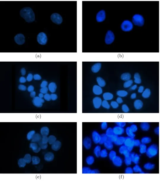
1.1 Example subimages of differently grown cells: (a), (b) are mono-layer/isolated cells that have no or very little contact with others; (c), (d) are touching cells that have an adjacent or a very close cell; (e), (f) are confluent cells which grow in aggregates and observed as overlapping objects in the image. The segmentation process gets more challenging from (a) to (f). . . 3 1.2 (a) An image of HepG2 hepatocellular carcinoma cell nuclei. (b)

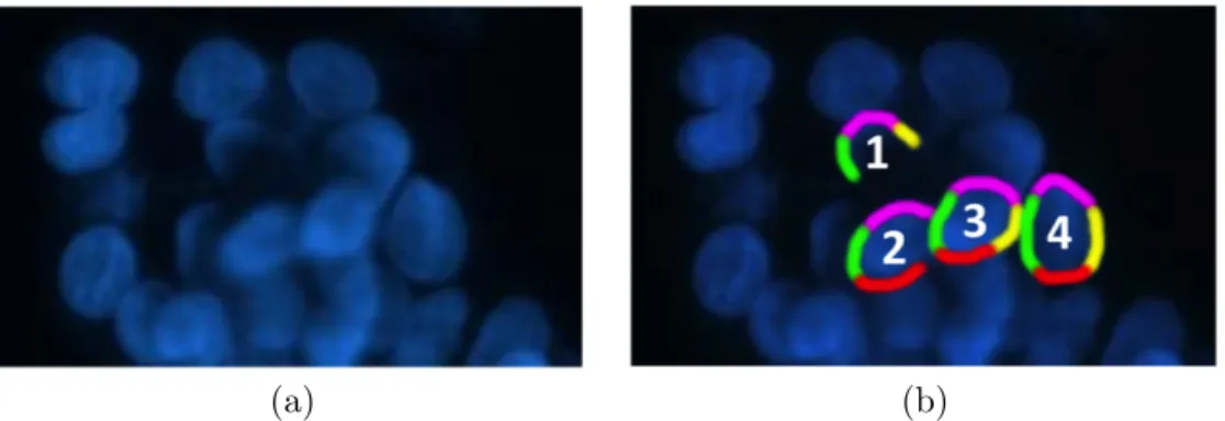
For four individual cell nuclei, the left, right, top, and bottom boundaries are shown as green, yellow, pink, and red, respectively. 4

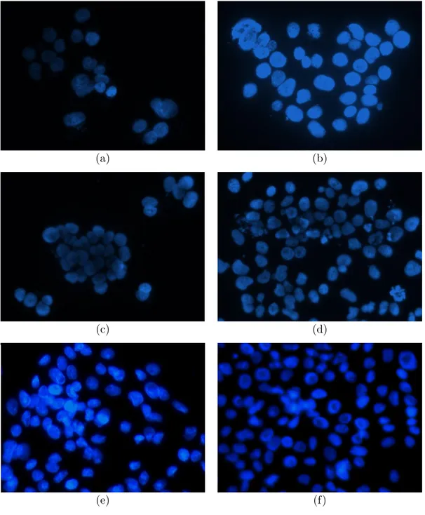
2.1 Several example fluorescence microscope image segments: (a), (c), (e) are taken from the HepG2 dataset; (b), (d), (f) are taken from the Huh7 dataset. The images evidently share some features such as color, bright foreground and dark background, but also show some differences in texture and illumination due to different cell lines and technical problems emerged during the image acquisition. 9 2.2 High content screening pipeline, which consists of image

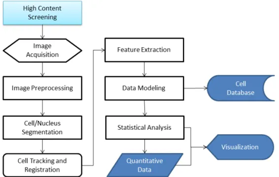
acquisi-tion, image preprocessing, cell/nucleus segmentaacquisi-tion, cell tracking and registration, feature extraction, data modeling and storage, statistical analysis, and visualization. . . 12

LIST OF FIGURES xi

2.3 Results of applying preprocessing methods to the image: (a) an example fluorescence image with high intensity variations and nonuniform shades due to uneven illumination, (b) the resulting image after preprocessing. . . 14 2.4 Illustrations of true, oversegmented, and undersegmented cells: (a)

a sample fluorescence microscopy image, (b) segmentation results, where oversegmented cells are annotated with red-cyan lines, un-dersegmented cells are annotated with red dotted lines, and true cells are annotated with yellow lines, (c) segmentation delineated by an expert, where each color represents a cell. . . 15 2.5 The results of applying global and local thresholding to an

exam-ple image: (a) a samexam-ple fluorescence microscopy image, (b) the segmentation result of global thresholding, (c) the segmentation result of local thresholding. Due to uneven illumination, global thresholding classifies relatively darker cellular pixels as background. 18 2.6 Illustration of how snakes work: (a) a sample fluorescence image,

(b) initial points provided around object boundaries, (c) initial boundaries, (d) final segmentation results. When initial points are given properly, the spline delineates the object boundaries, but with some limitations: (i) the spline may not localize concave curves accurately, (ii) touching cells may not be separated, which yields undersegmentation. . . 18 2.7 Illustration of active contours without edges: (a) a sample

fluores-cence image, (b) the randomly assigned first spline, (c) splines af-ter a few hundred iaf-terations, (d) final segmentation results. Active contours without edges can converge into boundaries regardless of the initial points. Contrary to the snakes as illustrated in Fig. 2.6, it better manages to separate touching cells. . . 19

LIST OF FIGURES xii

2.8 Illustration of a watershed in the field of image processing: (a) a synthetically generated gray scale image of two dark blobs, (b) 3D surface plot of the intensities where the colors of the points in the space turn into yellow as the intensity of the pixels increases. Start-ing from the minima (the darkest red), catchment basins merge onto the watershed line, illustrated with a dotted red line. . . 21 2.9 An example segmentation result obtained by a watershed

algo-rithm applied to only gradient magnitudes: (a) a sample fluores-cence image, (b) the gradient magnitudes, (c) 3D illustration of the gradient image, in which local minima can be observed around boundaries and the centroids of cells, (d) labeled segmented re-gions after applying watershed to the gradients. Since the flooding starts with all minima at the same time and catchment basins join as soon as they meet, the image is highly oversegmented. . . 22 2.10 An example to show that regional minima and suppressed minima

cannot handle oversegmentation problem when intensities are un-even: (a) gray-scale intensity image, (b) minima of the intensity image, (c) segmentation results using regional minima as markers, (d) suppressed regional minima via h-minima transform, (e) seg-mentation results using suppressed minima as markers. Although h-minima transform is used, the oversegmentation problem may still exist. Note that, for better illustration, a mask was used to eliminate noise in the background. . . 23

LIST OF FIGURES xiii

2.11 Integrating shape information in a marker-controlled watershed via distance maps: (a) the gray scale intensity map of the im-age in Fig. 2.9, (b) binary map obtained via Otsu’s thresholding method [1], (c) the inner distance transform map where the pixels around cell centroids have the furthest distance to the background, (d) reverse of the inner distance transform map where the regional minima corresponds to the markers, (e) the segmentation result af-ter applying marker-controlled waaf-tershed algorithm to the binary map. . . 23

3.1 Overview of the proposed algorithm. . . 26 3.2 Illustration of defining left boundary primitives: (a) original

subimage, (b) response map Rleft obtained by applying the

So-bel operator of left orientation, (c) mask that is to be used for determining local Sobel threshold levels, (d) binary image Bleft

af-ter thresholding, (e) boundaries obtained afaf-ter taking the leftmost pixels, (f) boundary map Pleft obtained after taking the d-leftmost

pixels, (g) Pleft after eliminating its smaller connected components,

(h) left boundary primitives each of which is shown with a different color. . . 27 3.3 Illustration of the benefits of using a mask: (a) original subimage,

(b) response map Rbottom obtained by applying the Sobel operator

of bottom orientation, (c) bottom boundary primitives obtained without a mask (a falsely detected primitive is marked with red), (d) bottom boundary primitives obtained with a mask. . . 29 3.4 Illustration of assignment of an edge between a left and a bottom

primitive: (a) primitives and (b) selected segments of the primitives. 30 3.5 Flowchart of the iterative search algorithm. . . 32

LIST OF FIGURES xiv

3.6 Two structural patterns used for cell localization: 4PRIM and 3PRIM patterns. Some instances of these patterns are shown in this fig-ure, indicating the corresponding edges with black and blue, re-spectively. Moreover, the 4PRIM pattern has two subtypes that correspond to subgraphs forming a loop (dashed black edges) and a chain (solid black edges). . . 33 3.7 Flowchart of the cell localization method. . . 34 3.8 Illustration of finding outermost pixels and calculating a radial

dis-tance ri. The primitive segments that lie in the correct sides of the

other primitives are identified and outermost pixels are selected. In this figure, unselected segments of the primitives are indicated as gray. . . 35 3.9 (a) Original subimage, (b) primitives identified for different cells,

and (c) cells delineated after the watershed algorithm. . . 36

4.1 Visual results on example subimages obtained by the proposed perceptual watershed algorithm and the comparison methods. The size of the subimages is scaled for better visualization. . . 42 4.2 For the Huh7 and HepG2 datasets, cell-based and pixel-based

F-score measures as a function of (a) the primitive length threshold tsize, (b) the percentage threshold tperc, (c) the standard deviation

threshold tstd, and (d) the radius W of the structuring element. . 46

4.3 For the Huh7 and HepG2 datasets, cell-based and pixel-based pre-cision measures as a function of (a) the primitive length threshold tsize, (b) the percentage threshold tperc, (c) the standard deviation

LIST OF FIGURES xv

4.4 For the Huh7 and HepG2 datasets, cell-based and pixel-based re-call measures as a function of (a) the primitive length threshold tsize, (b) the percentage threshold tperc, (c) the standard deviation

threshold tstd, and (d) the radius W of the structuring element. . 48

4.5 Visual results on example subimages obtained by the proposed perceptual watershed algorithm. . . 49 4.6 Visual results on example subimages obtained by the proposed

perceptual watershed algorithm. . . 50 4.7 Visual results on example subimages obtained by the proposed

perceptual watershed algorithm. . . 51 4.8 Visual results on example subimages obtained by the proposed

List of Tables

4.1 Comparison of the proposed perceptual watershed algorithm against the previous methods in terms of computed-annotated cell matches. The results are obtained on the Huh7 dataset. . . 43 4.2 Comparison of the proposed perceptual watershed algorithm

against the previous methods in terms of computed-annotated cell matches. The results are obtained on the HepG2 dataset. . . 43 4.3 Comparison of the proposed perceptual watershed algorithm

against the previous methods in terms of the cell-based precision, recall, and F-score measures. The results are obtained on the Huh7 dataset. . . 44 4.4 Comparison of the proposed perceptual watershed algorithm

against the previous methods in terms of the cell-based preci-sion, recall, and F-score measures. The results are obtained on the HepG2 dataset. . . 44 4.5 Comparison of the proposed perceptual watershed algorithm

against the previous methods in terms of the pixel-based preci-sion, recall, and F-score measures. The results are obtained on the Huh7 dataset. . . 44

LIST OF TABLES xvii

4.6 Comparison of the proposed perceptual watershed algorithm against the previous methods in terms of the pixel-based preci-sion, recall, and F-score measures. The results are obtained on the HepG2 dataset. . . 45

Chapter 1

Introduction

High content screening helps scientists analyze complex biological systems and collect quantitative data via automated microscopy imaging to improve the qual-ity of molecular biology research in means of speed and accuracy. In the last two decades, automated fluorescence microscopy imaging systems have become important tools, particularly in high content screening and drug discovery as they enable to carry out rapid high-throughput screening with better reproducibility. The first step of these systems typically includes cell/nucleus segmentation. It is the most critical part in cellular image analysis, since it greatly affects the success of the other system steps. Thus, it is of great importance to develop accurate segmentation algorithms, considering the requirements of a given problem. In different applications of the biology research, different types of cells that show different characteristics can be used. For example in drug discovery screening, it is essential to compare drug-treated cells with non-treated control cells for driving reliable assessment on the cytotoxic effects of the drug. The drug-treated cells mostly grow as monolayer isolated cells whereas the drug-free control cells usu-ally grow in aggregates on layers, which makes them more confluent. Thus, it is very critical for segmentation algorithms developed for drug discovery screening to operate on both isolated and confluent cells. Therefore, the proposed study in this thesis aims to develop such a cell segmentation method, which is capable of segmenting isolated and confluent cells.

1.1

Motivation

Standard drug discovery techniques require identifying the active compound by traditional methods, however, since molecular secrets about diseases have been revealed, it is now possible to find the compound that is responsible for the disease at molecular level. High throughput screening allows quantitative analysis in drug discovery by making possible to conduct thousands of experiments in a considerable amount of time. Especially the 2000s has been a golden era in the field, where efficient and effective methods have been developed in both academia and industry. Owing to increasing demands for newer and better applications, the research in the field is being evolved in a wide range and new solutions have been proposed both in software and hardware [2]. However, the tools to process and analyze the data are far away from perfection and they have still a lot of way to fulfill all the requirements in the field.

Although high content screening includes several steps to produce quantitative results, one of the major steps is the detection and segmentation of cells. Since the aim of the screening in drug discovery is to identify how drugs affect the phenotype of a cell, the importance of segmenting cells with a high accuracy is obvious. Therefore, in this study, we focus on cell detection and segmentation in fluorescence microscopy images.

In literature, there have been many studies proposed for cell/nucleus segmen-tation. These studies typically consider the specific characteristics of fluores-cence microscopy images, such as sharp intensity changes between cell nuclei and the background, to develop their algorithms. When the images mostly consist of monolayer isolated or less confluent cells, relatively simple methods such as thresholding [3, 4] are used to separate cell nuclei from the background. On the other hand, these methods are typically inadequate for segmenting more confluent cells that grow in aggregates. In that case, it has been proposed to use water-shed algorithms that operate on the intensity/gradient of image pixels and/or the shape information derived from a binary mask of the image [5, 6]. A typical problem of the watershed algorithms is over-segmentation. Marker-controlled wa-tersheds, which define a set of markers and let water rise only from these markers,

have been used to overcome this problem [7, 8, 9]. Moreover, the watershed al-gorithms usually refine their results by applying a merging or a splitting process to their segmented cells. They split or merge the segmented cells based on the properties of their regions as well as the similarity between the adjacent cells and their boundaries [10, 11].

(a) (b)

(c) (d)

(e) (f)

Figure 1.1: Example subimages of differently grown cells: (a), (b) are mono-layer/isolated cells that have no or very little contact with others; (c), (d) are touching cells that have an adjacent or a very close cell; (e), (f) are confluent cells which grow in aggregates and observed as overlapping objects in the image. The segmentation process gets more challenging from (a) to (f).

Although these previous studies lead to promising results, there still remain challenges to overcome for especially segmentation of confluent (clustered) cells. To make the isolated and confluent cells concepts more clear, we present some example images of cell groups in Fig. 1.1. The figure reveals that it is relatively easier to segment isolated (a, b) and touching cells (c, d). On the other hand, segmentation of confluent cells (e, f) needs a great effort, but not usually for human eyes. The main challenge in segmenting objects actually lies in the na-ture of the problem. Cell segmentation, like all other segmentation problems, is closely related with human perception. Humans typically use their perceptions in handling noise and variations in an image as well as in separating confluent cells from each other.

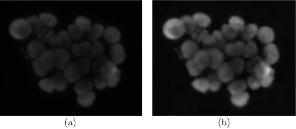
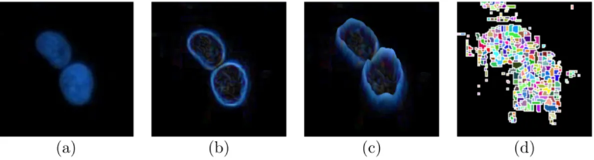
(a) (b)

Figure 1.2: (a) An image of HepG2 hepatocellular carcinoma cell nuclei. (b) For four individual cell nuclei, the left, right, top, and bottom boundaries are shown as green, yellow, pink, and red, respectively.

In this thesis, we introduce a new marker-controlled watershed algorithm that incorporates human perception into cell segmentation. This “perceptual water-shed” algorithm relies on modeling a very trivial fact that a human uses: each cell should have a left boundary, a right boundary, a top boundary, and a bottom boundary and these boundaries should be in the correct position with respect to each other. Fig. 1.2 illustrates these boundaries for four individual cell nuclei with the left, right, top, and bottom boundaries being shown as green, yellow, pink, and red, respectively. In the figure, one can observe that the bottom (red) boundary of Cell 1 is not identified due to an uneven lighting condition. Similarly, the right (yellow) boundary of Cell 2 is not present in the image due to its partial overlapping with Cell 3. However, it is possible to identify these two cells by

using only their present boundaries and the spatial relations of these boundaries. Moreover, here it is obvious that the green boundary of Cell 3 cannot belong to Cell 2, but it reveals the fact that Cell 3 is overlapping with Cell 2. On the other hand, the boundaries of Cell 3 and Cell 4 form close shapes, which make them easy to separate from the background. In this thesis, such observations are our main motivations behind implementing the proposed perceptual watershed algorithm.

1.2

Contribution

In the proposed algorithm, our contributions are three-fold: First, we represent cell boundaries (left, right, top, and bottom) by defining four different types of primitives and represent their spatial relations by constructing an attributed re-lational graph on these primitives. Second, we reduce the marker identification problem to the problem of locating predefined structural patterns on the con-structed graph. Third, we make use of the boundary primitives to guide the flooding process in the watershed algorithm. The proposed algorithm mainly differs from the previous cell segmentation algorithms in the following aspect. Instead of directly working on image pixels, our algorithm works on high-level boundary primitives that better correlate with the image semantics. The use of the boundary primitives help better separate confluent cells. Moreover, this use is expected to be less vulnerable to noise and variations that are typically observed at the pixel level. Working on a total of 2661 cells in two datasets, our experiments demonstrate that the proposed perceptual watershed algorithm, which uses the boundary primitive definition, improves the segmentation of fluo-rescence microscopy images by locating better markers and obtaining better cell boundaries for both less and more confluent cells, compared to its counterparts.

1.3

Outline

The structure of this thesis is as follows. In Chapter 2, we introduce a brief de-scription of the problem domain including the molecular biological background of this study and specific characteristics of fluorescence microscopy images. We end up the chapter by introducing high content screening with its sub-steps and sum-marize existing approaches from the literature for cell/nucleus segmentation. In Chapter 3, we give the details of our proposed cell segmentation method including the primitive definition, graph construction, cell localization (marker identifica-tion), and region growing steps. In Chapter 4, we present our experimental results with the explanation of datasets, test environment, comparison methods, and parameter analysis. In Chapter 5, we finalize the thesis with a conclusion and discuss the future work.

Chapter 2

Background

2.1

Domain Description

In this section, we introduce a brief description of fluorescence microscopy and the specific characteristics of fluorescence microscopy images. Moreover, we discuss the difficulties in fluorescence microscopy imaging, which have a negative effect on the performance of the segmentation process. The section is ended up with some information about the cell lines used throughout this study and basic preparation details of the specimens before taking the images.

2.1.1

Fluorescence Microscopy Images

Fluorescence microscopy has been a very functional technology in both biological and medical areas. The name “fluorescence microscope” origins from its work-ing principle, in which fluorescence is made use of to generate an image. The specimen that is wanted to be studied is fluoresced so that it can emit the light with a specific wavelength while sorting out the others. Here, the key is usage of filters which only allow the desired wavelength to pass and block the rays of light with undesired wavelengths [12]. Since the specimen is radiated by fluo-rescence, cellular regions are observed in the microscope to shine out on a dark

background with a high contrast. This high contrast between the foreground and the background arises as sharp intensity changes on the taken images, therefore it becomes possible to identify the cellular regions clearly. In Fig. 2.1, several example fluorescence microscopy images are given, where specific characteristics of the images can be observed clearly.

Separation of cellular regions from the background is relatively easy due to aforementioned characteristics of fluorescence microscopy images. On the other hand, a critical factor for the performance of the segmentation task is the quality of the images. Noise and uneven illumination turn up to be the biggest draw-backs during the segmentation process. These drawdraw-backs mainly arise due to technical issues related with the hardware (a microscope and a camera) and/or the specialist. The focus level of the objective, the effects of the filters, the illu-mination of the image as well as the setup of the hardware and the experiment play a critical role for obtaining images of high quality. The adjustments should be set in a careful manner, which is directly related with the expertise of the spe-cialist. Moreover, if the image taking process is handled manually, the handiness of the expert who captures the images is also very important. All these factors may result to good-quality, clear, and well-focused images or bad-quality, noisy, and shaded images, which make a huge difference for an accurate segmentation process and the further analysis. An example of uneven illumination is shown in Fig. 2.1(a) and Fig. 2.1(c). A robust segmentation algorithm should be capable of handling such problems or minimize their effects.

The structure of cells, on the other hand, is another factor that may affect the quality of images. Similar to high contrast between cells and the background, the subcellular objects in the cytoplasm and some artifacts related to the specimen may also have a textural difference inside the cells. Although they may be useful as an indicator for identifying cells, they may also mislead the algorithm, which results in false detection of a bright pixel out of a cellular region or oversegmen-tation. Thus, these artifacts are considered as noise and should be avoided to increase the accuracy of the algorithm. An example noisy image is presented in Fig. 2.1(d).

(a) (b)

(c) (d)

(e) (f)

Figure 2.1: Several example fluorescence microscope image segments: (a), (c), (e) are taken from the HepG2 dataset; (b), (d), (f) are taken from the Huh7 dataset. The images evidently share some features such as color, bright foreground and dark background, but also show some differences in texture and illumination due to different cell lines and technical problems emerged during the image acquisi-tion.

Another roadblock in automated cell segmentation via fluorescence mi-croscopy lies on the nature of cell behavior. Although, for example the treated cells in drug screening tend to grow in monolayers, cells naturally grow in ag-gregates. As they continue to grow and divide, the confluency of the cells in-crease simultaneously, resulting in a more dense image. Therefore, segmenting overlapping cells turns to be a harder problem compared to segmenting mono-layer/isolated cells (see Fig. 1.1).

2.1.2

Cell Lines

In this study, we used two set of images, taken from human hepatocellular carci-noma (HCC) cell lines (Huh7 and HepG2). Sample preparation and image acqui-sition took place at the Molecular Biology and Genetics Department of Bilkent University. The cells were cultured routinely at 37◦C under 5% CO2 in a standard

medium (DMEM) supplemented with 10% FCS. To visualize the selenium defi-ciency or drug dependent morphological changes in HCC cells, cells were seeded on autoclave-sterilized coverslips in 6-well plates and cultured overnight in the standard medium. Next day, for the induction of cell death through selenium deficiency dependent oxidative stress, cells were exposed to a selenium-deficient (HAM’s medium with 0.01% FCS) or a selenium-supplemented (HAM’s medium with 0.01% FCS and 0.1 µM sodium selenite (Sigma)) medium. Cells were main-tained in these media for up to 10 days by refeeding with fresh media every 2 days. For the visualization of cell death through drug-induced cytotoxicity, cells seeded on 6-well plates were supplemented with fresh media after overnight cul-ture and were treated with two well-known cell death inducing drugs Adriamycin (1 µg/ml) and Camptothecin (5 µM) for 48h.

During the experiments, cell morphology changes were observed under an in-verted microscope. To determine nuclear condensation by Hoechst 33258 (Sigma) staining, coverslips were washed with ice-cold PBS twice and fixed in 70% (v/v) cold ethanol for 10 min. After incubation with 1µg/ml Hoechst 33258 for 5 min in the dark, coverslips were destained with ddH2O for 10 minutes and mounted on glass microscopic slides in 50% glycerol, to be examined under a Zeiss Axioskop

fluorescent microscope.

2.2

High Content Screening

High content screening fuses the efficiency of high-throughput techniques with fluorescence microscopy imaging to process and analyze large datasets in a con-siderable amount of time. The produced quantitative output accelerates the decision-making process in molecular cellular biology research, particularly in drug discovery. Development of efficient and effective algorithms and latest ad-vances in hardware are the key points behind the high-throughput capability of high content screening tools. On the other hand, the whole system’s performance is directly dependent on the effectiveness of sub-systems, each of which has its own importance for qualified analysis.

High content screening typically consists of independent sub-steps, all of which aim to solve specific problems [13]. These sub-steps include acquisition of the images, image preprocessing, cell/nucleus segmentation, cell tracking and regis-tration, feature extraction, data modeling and storage, statistical analysis, and visualization. Figure 2.2 summarizes the flow of the process in a typical high content screening tool.

The image acquisition step provides fluorescence microscopy images that will be processed throughout the system to extract quantitative data. The quality of the images is very critical for better segmentation and consistent feature extrac-tion (refer to Sec. 2.1.1 for more informaextrac-tion). Unfortunately no imaging system is perfect, thus the images probably would suffer from noise and/or uneven shad-ing. To reduce the negative effects of uneven illumination, image preprocessing techniques are applied to the images, such as contrast enhancement and noise removal. Next, cell segmentation takes place, which is the core step in image analysis, since the performance of next sub-steps are very dependent on the ac-curate segmentation of cells. The aim of cell segmentation process is to identify

Figure 2.2: High content screening pipeline, which consists of image acquisition, image preprocessing, cell/nucleus segmentation, cell tracking and registration, feature extraction, data modeling and storage, statistical analysis, and visualiza-tion.

and separate interest areas, so that cell features can be extracted and quantita-tive experiments can be conducted on them. Cell segmentation is usually followed by cell tracking and registration in many applications since examining the cell behavior, such as mitosis and the phenotype of a cell would be of high value. Tracking directly works on segmented objects and attempts to associate possible divided cells according to some criteria such as the speed of motion, the shape of the trajectory, and the possibility of being divided from the same parent [14].

After acquiring the cells and tracks between them, the image processing part finishes and the data analysis part starts. For that, the first step is extract-ing some numeric data to describe cell specific features for further analysis. A variety of features such as area, shape, size, perimeter, intensity, texture, and pattern are widely used to classify different types of cells [15]. On the other hand, track specific features such as the change of the size and shape of the cell during and after mitosis can be useful to identify the track or the behaviour of

a cell [13]. After feature extraction, the high amount of data should be orga-nized and archived properly in a well designed database for statistical feature analysis, cell classification, and data mining, so that valuable information would be extracted. Visualization is also an important step to clearly represent the information gained throughout these processes.

Details of the cell segmentation step and state-of-the-art algorithms as well as some brief information about image preprocessing will be given in the following subsections, while other system steps are not in the scope of this thesis. More information about high content screening is briefly given in [13, 16, 14].

2.2.1

Image Preprocessing

Image preprocessing refers to a series of techniques to improve the quality of raw images before further processing such as segmentation and feature extrac-tion [13]. There exist various preprocessing techniques [17, 18], however the most useful ones for fluorescence microscopy images are noise removal and contrast enhancement.

High amount of intensity variations and nonuniform shades caused by uneven illumination are not desired in images, since they directly affect the performance of image analysis. Besides, the noise, which adds spurious and extraneous infor-mation to the images, is also an important problem especially for fluorescence microscopy images (see Sec. 2.1.1). Therefore, the effects of uneven illumination and noise in the images should be reduced before continuing through further processes. Fig. 2.3 illustrates the positive effects of enhancement on a sample fluorescence microscopy image. After processing the image in Fig. 2.3(a), it is observable that the amount of uneven shades reduces in Fig. 2.3(b), while the edges of the inner cells become more clear.

Contrast enhancement, also called shade correction, is the process of correct-ing illumination artifacts and reduccorrect-ing intensity variations in the images. An

(a) (b)

Figure 2.3: Results of applying preprocessing methods to the image: (a) an example fluorescence image with high intensity variations and nonuniform shades due to uneven illumination, (b) the resulting image after preprocessing.

iterative method for this purpose is based on B-spline estimation of the back-ground which improves the quality of the image in each iteration by subtracting the estimated B-splines from the original image [19, 20]. Histogram equaliza-tion is another method for contrast adjustment, which distributes the intensi-ties more evenly, therefore reduces the amount of intensity variations in the im-ages [21, 22]. Besides, it is also possible to apply filters beforehand for enhancing the images [23, 24, 6].

Noise removal is the process of eliminating undesired stains, spots, and arti-facts from the images, which emerge due to specimen or instruments used while acquiring the images. Noise removal techniques are usually based on convolution, in which a filter or a kernel is convolved on the image removing the noise and smoothing the objects in local segments. Popular techniques used for this pur-pose include Gaussian filtering [11, 5], median filtering [25, 26, 20], morphological opening [27], and windows slicing [10].

2.2.2

Cell/Nucleus Segmentation

The first step in cellular image analysis is automatic detection and identification of cells/nuclei. For this aim, cells have to be separated from the background by specific image processing techniques. It is in the heart of the cellular image

analysis, regardless of the application area. The accuracy of segmentation process directly affects the results of the study, since the subsequent steps of the analysis are highly dependent on the segmented cells. Therefore, cell segmentation is one of the most intensely studied problems in cellular image analysis. While a robust and general method for cell segmentation is desired in the area, it is difficult to model a generic strategy with the ability to work for all types of cellular images. Therefore, various methods have developed using the information extracted from different characteristics of the images.

The high contrast between fluoresced cells and the dark background leads to sharp intensity changes in the images. These properties play a primary role in the design of cell segmentation methods for fluorescence microscopy. On the other hand, cell segmentation is an ill-posed problem, therefore the frame of the problem should be delineated clearly and the algorithm should make use of the specific characteristics of the images together with the domain knowledge. Otherwise, cells may not be segmented properly or even may not be detected. The segmented regions labeled as cells may correspond to more than one actual cell, which is called undersegmentation, or an actual cell may further be segmented into subregions, which is called oversegmentatition. In Fig. 2.4 true, oversegmented, and undersegmented results are illustrated for better understanding.

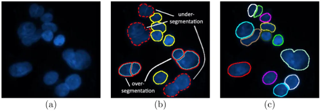
(a) (b) (c)

Figure 2.4: Illustrations of true, oversegmented, and undersegmented cells: (a) a sample fluorescence microscopy image, (b) segmentation results, where overseg-mented cells are annotated with red-cyan lines, undersegoverseg-mented cells are anno-tated with red dotted lines, and true cells are annoanno-tated with yellow lines, (c) segmentation delineated by an expert, where each color represents a cell.

Well known techniques that focus on the segmentation problem in fluores-cence microscopy images include thresholding, active contours, and watershed-based methods. These methods are usually applied on preprocessed images to increase the quality of segmentation and followed by a post-process to refine the segmentation results. The following sections will briefly explain the methods and the-state-of-the-art algorithms in the literature of cellular image analysis, with their weak and strong points. On the other hand, this thesis commonly focuses on the methods specifically designed for cell/nucleus segmentation. A more exten-sive study on image segmentation [28] and a survey on segmentation algorithms developed for the medical field [29] can give a deeper understanding to the reader.

2.2.2.1 Thresholding

Thresholding is the simplest method to differentiate foreground objects and the background. The simple idea behind the method is classifying each grayscale pixel according to a predefined threshold. If the intensity of the pixel is above the threshold, it is classified as a foreground pixel, otherwise it is classified as background. Let I be the intensity image and t be the threshold value. The binary image B obtained via thresholding is defined as:

B(i, j) = (

1 if I(i, j) > t

0 otherwise. (2.1) The key point here is the selection of the right threshold. For a better differen-tiation, a threshold should be preferred which maximizes the inter-class variance and minimizes the intra-class variance between the foreground objects and the background [13]. The threshold may be computed globally, in which the entire image is used [1] or, adaptively, where the threshold is computed using the local information gained from the sub-regions of the image [30]. A detailed study on image thresholding methods is presented in [31].

shine out on a relatively darker background. Therefore, it is easy to differenti-ate the cellular regions and the foreground via thresholding. If an image contains mostly monolayer isolated cells, finding connected components on the binary map is usually sufficient to locate the cells. However, when the image contains conflu-ent cells as well, thresholding usually leads to undersegmconflu-entation (Fig. 2.4(b)). To overcome this problem, more complex techniques are necessary to separate the confluent cells and these techniques can use the binary map in the subse-quent system steps (for instance, the binary map is used to calculate a distance transform for the watershed algorithm, which will be shortly covered in 2.2.2.3). Therefore, for fluorescence microscopy images, the thresholding result is generally used as a binary map or a mask for more sophisticated segmentation algorithms, rather than identifying individual cells [32, 3, 33, 34].

When the image is uniformly illuminated, it is well known that global thresh-olding [35, 36] is a simple and good way to obtain a binary map that differentiates cellular regions and the image background. On the other hand, applying global thresholding on images caused with uneven illumination usually does not lead to desired results. To overcome this, local (adaptive) thresholding is used, so that pixels are classifed according to locally calculated thresholds so that the other parts of the image are not affected [4, 37, 38]. In Fig. 2.5, the results of applying global and local thresholding to a sample image is illustrated. The figure reveals that local thresholding is always one step forward from global thresholding when the image is not uniformly illuminated.

2.2.2.2 Active Contour Based Methods

Active contours, also called snakes and deformable models [39], have been widely used to delineate the object outline since they first introduced in [40]. An active contour is a spline, localized to an object boundary by minimizing its energy function. This function is defined on internal forces that control the smoothness of the boundary as well as external forces that pull the boundary towards the object’s gradient. The dynamic behaviors of active contours give them the abil-ity to find the object boundaries even in noisy environment. It is also possible to

(a) (b) (c)

Figure 2.5: The results of applying global and local thresholding to an example image: (a) a sample fluorescence microscopy image, (b) the segmentation result of global thresholding, (c) the segmentation result of local thresholding. Due to uneven illumination, global thresholding classifies relatively darker cellular pixels as background.

increase the power of snakes by introducing different energy functions [41]. On the other hand, it is very critical for snakes to start with a good initial spline for obtaining good final results. Most of the time, the initial spline points near the object boundary are provided by a user interface or approximate object co-ordinates are given to the snake by an initial segmentation map. How snakes converge into object boundaries is illustrated on a sample fluorescence image in Fig. 2.6.

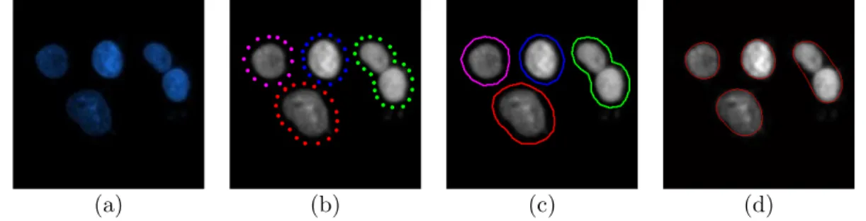
(a) (b) (c) (d)

Figure 2.6: Illustration of how snakes work: (a) a sample fluorescence image, (b) initial points provided around object boundaries, (c) initial boundaries, (d) final segmentation results. When initial points are given properly, the spline delineates the object boundaries, but with some limitations: (i) the spline may not localize concave curves accurately, (ii) touching cells may not be separated, which yields undersegmentation.

Active contours have been fully automated since gradient vector flow was introduced [42] to guide the spline as an external force. This allows the active

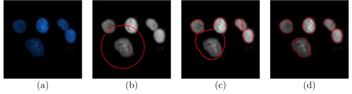
(a) (b) (c) (d)

Figure 2.7: Illustration of active contours without edges: (a) a sample fluorescence image, (b) the randomly assigned first spline, (c) splines after a few hundred iterations, (d) final segmentation results. Active contours without edges can converge into boundaries regardless of the initial points. Contrary to the snakes as illustrated in Fig. 2.6, it better manages to separate touching cells.

contour to find its way through the interest points. Furthermore, the effectiveness of active contours upgraded to a higher level when their dependencies on the gradient were broken by active contours without edges [43]. It is a single level set algorithm that divides the image into two regions. The spline is evolved by the average intensity that is computed from the segmented regions that remain inside and outside of it. The method gives quite accurate results even if foreground objects show similar textural properties. Moreover, neither the initial curve needs to be around the object boundaries, nor it should be initialized externally. The segmentation process handled by active contours without edges is illustrated in Fig. 2.7.

Deformable shapes of cells and intensity variations in the images are very suited to be modeled by active contours, thus several active contour based models were adapted to solve the cell segmentation problem in fluorescence microscopy images. Some of them follow an updated way of the traditional active contours which rely on the gradient [44, 45, 46] or the intensity [47]. The snake-based methods make use of a binary map obtained via thresholding [45], a modified version of the gradient vector flow [46], or a mixture of them [44] to initialize object boundaries for curve evolution while the region-based methods rely on a level set based active contour algorithm [47]. The common point of these studies is the affinity of the images where the cells have strong gradients which differentiate them from the background and the other objects.

On the other hand, traditional active contour models do not yield good re-sults when images mostly consist of overlapping or touching cells, so that, they tend to merge adjacent boundaries into single objects. In order to overcome this drawback, a multiphase extension of a traditional single level set method [48], that defines logn level set functions for n phases has been presented in [20]. Sev-eral studies carried this idea further by defining level set functions for every cell on the initial segmentation map and defining coupling constraints to prevent ad-jacent cells from merging [49, 50, 51]. The reason behind using different level sets for every cell is that the average intensities inside cells do not need to be equal. Thus, objects with different average intensities are segmented more accu-rately. Moreover, by assigning penalties to contour overlaps, merging of adjacent cells is avoided. Different from its ancestor, multiphase level set methods need initial contours, which may be obtained via thresholding [20] or an automatic initialization using a single level set function [49].

2.2.2.3 Watershed Based Methods

For more than two decades, watershed algorithms have been one of the primary tools for image segmentation [52, 53, 54]. The method is inspired from water-sheds of the field of topography, which are geographical boundaries (i.e., ridges) that divide adjacent catchment basins [53]. In mathematical morphology [55], gray-scale intensity images or gradient magnitudes can be interpreted as topo-graphic surfaces, in which bright and dark pixels correspond to hills and hollows, respectively. Each intensity or gradient in the image represents the altitude of that point in the landscape where the peaks are the pixels with high intensities, or high gradients (i.e., the edges of the objects), and vice versa. To better un-derstand the watershed algorithm, imagine that a rain starts over the landscape, filling the minima with water. As the water rises, water in adjacent catchment basins meet and the points where two catchment basins join each other form a watershed which, at the end, corresponds to the segmented object boundaries. In Fig. 2.8, the immersion of the landscape and the formation of the watersheds are illustrated.

(a) (b)

Figure 2.8: Illustration of a watershed in the field of image processing: (a) a synthetically generated gray scale image of two dark blobs, (b) 3D surface plot of the intensities where the colors of the points in the space turn into yellow as the intensity of the pixels increases. Starting from the minima (the darkest red), catchment basins merge onto the watershed line, illustrated with a dotted red line.

Watershed-based algorithms are of great importance to handle the cell seg-mentation problem. Thresholding and deformable models work well on images that mostly consist of monolayer isolated or touching cells, but their power weak-ens on the clustered/overlapped nuclei, which typically leads to undersegmented results. Therefore, when nuclei are clustered and/or have fuzzy boundaries, tershed based algorithms come into play. On the other hand, applying the wa-tershed algorithm to only gray-scale intensities or gradient magnitudes always almost leads to oversegmentation due to regional minima in both objects (cells) and the background. The flooding operation starts from the regional minima all over the image, and regardless of their levels, a watershed line is formed as soon as two floods meet, resulting in more segmented objects than expected. An example segmentation result obtained by a watershed algorithm applied to only gradient magnitudes is illustrated in Fig. 2.9. Since regional minima emerge from uneven gradients near boundaries and the centroids of cells, the process ends up with oversegmentation.

A common solution to handle this problem is assigning seed points, instead of letting the flood start from regional minima. This method is called marker-controlled watershed, since the regions start to grow only from previously iden-tified seed points (markers) and the flow of the flood is controlled by a marking function. But this gives another important question: How should one define

(a) (b) (c) (d)

Figure 2.9: An example segmentation result obtained by a watershed algorithm applied to only gradient magnitudes: (a) a sample fluorescence image, (b) the gradient magnitudes, (c) 3D illustration of the gradient image, in which local minima can be observed around boundaries and the centroids of cells, (d) labeled segmented regions after applying watershed to the gradients. Since the flooding starts with all minima at the same time and catchment basins join as soon as they meet, the image is highly oversegmented.

markers so that each of them matches with an existing object? The answer to this question hides under the problem itself. Since oversegmentation occurs due to high number of spurious minima, it would be reasonable to eliminate them. For that, h-minima transform is a widely used method that suppresses undesired minima on the image [7, 56, 11]. On the other hand, applying h-minima transform to reduce the number of false minima does not help solve the oversegmentation problem when gradients or intensities are severely uneven. An example cell that shows such characteristics is given in Fig. 2.10(a). When h-minima applied to the image (Fig. 2.10(d)) the amount of over partitioned parts is highly reduced (Fig. 2.10(e)) compared to the segmentation results where only regional minima are used (Fig. 2.10(c)), but the oversegmentation problem still exists.

Another approach for marker definition is to make use of a priori shape infor-mation captured via initially segmenting the image [32, 3]. This initial segmen-tation result, usually referred as a binary map or mask, would be used for marker identification [33, 34]. It is also used for marking function definition [7, 57] to cover all cellular regions so that while the markers are growing the intrusion of floods to other cells and the background are avoided.

One of the widely used methods to integrate the shape information into a marker controlled watershed algorithm is inner distance transform [25, 8]. In

(a) (b) (c) (d) (e)

Figure 2.10: An example to show that regional minima and suppressed min-ima cannot handle oversegmentation problem when intensities are uneven: (a) gray-scale intensity image, (b) minima of the intensity image, (c) segmentation results using regional minima as markers, (d) suppressed regional minima via h-minima transform, (e) segmentation results using suppressed h-minima as markers. Although h-minima transform is used, the oversegmentation problem may still exist. Note that, for better illustration, a mask was used to eliminate noise in the background.

this transform, for each pixel in the foreground, a value is assigned which is the distance to the nearest zero pixel of the mask, as illustrated in Fig. 2.11. Inner distance transform ensures that the pixels around the centroids get the furthest distances to the background. Reversing the inner distance map (Fig. 2.11(d)), the furthest distances turn up to be the regional minima (or regional maxima for the inner distance transform) in the map, which can be used as markers for the watershed algorithm [58, 7]. Besides, to better deal with the problem, it is also possible to combine shape information with gradient/intensity information [58, 11, 21].

(a) (b) (c) (d) (e)

Figure 2.11: Integrating shape information in a marker-controlled watershed via distance maps: (a) the gray scale intensity map of the image in Fig. 2.9, (b) binary map obtained via Otsu’s thresholding method [1], (c) the inner distance transform map where the pixels around cell centroids have the furthest distance to the background, (d) reverse of the inner distance transform map where the regional minima corresponds to the markers, (e) the segmentation result after applying marker-controlled watershed algorithm to the binary map.

Another way of using cellular shapes for marker definition is to apply morpho-logical operations to the mask of an image. One of the classical approach for that is using ultimate eroding points as seed points [17]. But since it is inadequate to oversegmentation, iterative approaches have been proposed in which morpho-logical erosion is applied to the binary map of the image by a series of cell-like structural elements to identify markers, while preserving their shapes [9, 59].

Marker-controlled watersheds give accurate results if there is one-to-one map-ping between the markers and the actual cells. Otherwise, they may result in under- or over-segmentation. To address this problem, many studies post-process the segmented cells that are obtained by their watershed algorithms. This post-processing relies on extracting features from the segmented cells and the bound-aries of the adjacent ones and using these features to validate, merge, or split the cells. For that, they use score-based [26, 25, 6], rule-based [10, 60, 33], and iterative [38, 61, 62] techniques.

2.2.2.4 Other Methods

Besides thresholding, deformable models and the watersheds, shape-based and graph-based methods can be used for segmentation. The shape-based methods use the fact that cells typically have round and convex shapes. For that, they locate circles/ellipses on the binary map of the image to find the initial cell bound-aries and refine them afterwards [63, 27]. Alternatively, they find concave points on the binary map and split the map into multiple cells from these points [64, 65]. In cell segmentation studies, graphs are commonly used to merge the overseg-mented cells by constructing a graph over the adjacent ones [25, 66] as well as to refine initial segmentation results through the graph cut algorithms [67, 68, 69]. On the other hand, our segmentation method is different than these previous studies in the sense that it uses graphs to represent the spatial relations of the high-level boundary primitives and to define the markers of a watershed algo-rithm. Note that besides segmentation, it is also possible to use graphs for cell tracking applications [70, 71, 72], which are beyond the scope this thesis.

Chapter 3

Methodology

The proposed algorithm relies on modeling cell nucleus boundaries for segmen-tation. In this model, we approximately represent the boundaries by defining high-level primitives and use them in a marker-controlled watershed algorithm. This watershed algorithm employs the boundary primitives in its two main steps: marker identification and region growing. The marker identification step is based on using the spatial relations among the primitives. For that, we first construct a graph on the primitives according to their types and adjacency. Then, we use an iterative search algorithm that locates predefined structural patterns on the constructed graph and identify the located structures as markers provided that they satisfy the shape constraints. The region growing employs the primitives in its flooding process. Particularly, it decides in which direction it grows and at which point it stops based on the primitive locations. An overview of the pro-posed method is given in Fig 3.1. The details of these steps are explained in the next subsections.

3.1

Primitive Definition

In the proposed method, we define four primitive types that correspond to left, right, top, and bottom cell nucleus boundaries. These boundary primitives are

Figure 3.1: Overview of the proposed algorithm.

derived from the gradient magnitudes of the blue band Ibof an image. To this end,

we convolve the blue band Ib with each of the following Sobel operators, which

are defined in four different orientations, and obtain four maps of the responses. Then, we process each of these responses, as explained below and illustrated in Fig. 3.2, to define the corresponding primitives.

   −1 0 1 −2 0 2 −1 0 1       1 0 −1 2 0 −2 1 0 −1       −1 −2 −1 0 0 0 1 2 1       1 2 1 0 0 0 −1 −2 −1   

Let Rleft be the response map obtained by applying the Sobel operator of left

orientation to the blue band image Ib. We first threshold Rleft to obtain a binary

left boundary map Bleft. Here we use local threshold levels instead of using a

(a) (b) (c) (d)

(e) (f) (g) (h)

Figure 3.2: Illustration of defining left boundary primitives: (a) original subim-age, (b) response map Rleft obtained by applying the Sobel operator of left

ori-entation, (c) mask that is to be used for determining local Sobel threshold levels, (d) binary image Bleftafter thresholding, (e) boundaries obtained after taking the

leftmost pixels, (f) boundary map Pleft obtained after taking the d-leftmost

pix-els, (g) Pleftafter eliminating its smaller connected components, (h) left boundary

primitives each of which is shown with a different color.

images. For that, we employ a mask that roughly segments cellular regions from the background. For each connected component C(k) _{of this mask, we calculate a}

local threshold level T_left(k)on the gradients of its pixels by using Otsu’s method [1]. Then, pixels of this component are identified as boundary if their responses are greater than the calculated local threshold.

Next, we fill the holes in Bleft and take its d-leftmost pixels. The map Pleft of

the d-leftmost pixels are defined as:

Pleft(i, j) =       

1 if Bleft(i, j) = 1 and

∃x ∈ Z+ _{s.t. x ≤ d and B}

left(i − x, j) = 0

0 otherwise.

(3.1)

In this definition, the d-leftmost pixels are taken instead of just taking the leftmost pixels. The reason is that, as illustrated in Fig. 3.2(e), the leftmost pixels do not always contain all of the cell boundaries, and thus, there may exist discontinuities between the boundaries of the same cell. On the other hand, by taking the d-leftmost pixels, it is more likely to eliminate the discontinuities, as

shown in Fig. 3.2(f). Finally, we eliminate the connected components of Pleft

whose height is less than a threshold tsize and identify the remaining ones as left

boundary primitives. For an example subimage, Fig. 3.2(h) shows the identified left primitives with different colors.

Likewise, we define the right boundary primitives Pright, top boundary

primi-tives Ptop, and bottom boundary primitives Pbottom. In each of these definitions,

Eqn. 3.1 is modified as follows:

Pright(i, j) =       

1 if Bright(i, j) = 1 and

∃x ∈ Z+ _{s.t. x ≥ d and B} right(i + x, j) = 0 0 otherwise. (3.2) Ptop(i, j) =       

1 if Btop(i, j) = 1 and

∃x ∈ Z+ _{s.t. x ≤ d and B} left(i, j − x) = 0 0 otherwise. (3.3) Pbottom(i, j) =       

1 if Bbottom(i, j) = 1 and

∃x ∈ Z+ _{s.t. x ≥ d and B}

bottom(i, j + x) = 0

0 otherwise.

(3.4)

Eqn. 3.2, Eqn. 3.3 and Eqn. 3.4 give the rightmost, topmost, and d-bottommost pixels, respectively. Besides, in the elimination of smaller primitives, the components whose height is less than the threshold tsize are eliminated for

Pleft and Pright whereas those whose width is less than tsizeare eliminated for Ptop

and Pbottom.

In this step, we use a mask to calculate local threshold levels. This mask roughly identifies the cellular regions but does not provide their exact locations. Here our framework allows using different binarization methods such as adaptive thresholding [37] and active contours without edges [43]. However, since this mask is used just for calculating the local thresholds, we prefer using a relatively

simpler method. In this binarization method, we first suppress local maxima of the blue band image Ib by subtracting its morphologically opened image from

itself. This process removes the noise from the image without losing local intensity information. Then, we calculate a global threshold level on the suppressed image using the Otsu’s method [1]. In order to ensure that almost all of the cellular regions are covered by the mask, we decrease the calculated level to its half and threshold the suppressed image. Finally, we eliminate small holes and regions from the mask. The benefits of using a mask is illustrated in Fig. 3.3. Global thresholding of the entire image leads to loss of information, thus one can get more accurate results by considering only pixels of interest. The binary mask also avoids spurious bright pixels inside cellular regions.

(a) (b)

(c) (d)

Figure 3.3: Illustration of the benefits of using a mask: (a) original subimage, (b) response map Rbottom obtained by applying the Sobel operator of bottom

orientation, (c) bottom boundary primitives obtained without a mask (a falsely detected primitive is marked with red), (d) bottom boundary primitives obtained with a mask.

3.2

Marker Identification

Markers are identified by first constructing a graph on the primitives and then applying an iterative algorithm that searches this graph to locate structural pat-terns conforming to the predefined constraint. In the following subsections, we will explain the graph construction step and the iterative search algorithm.

3.2.1

Graph Construction

Let G = (V, E) be a graph constructed on the primitives V = {Pleft, Pright,

Ptop, Pbottom} that are attributed with their primitive types. An edge e = (u, v) ∈

E is assigned between primitives u and v if they satisfy the following three con-ditions:

1. The primitives should have overlapping or adjacent pixels.

2. One primitive should be of the vertical (left or right) type and the other should be of the horizontal (top or bottom) type.

3. Each primitive should have a large enough segment that lies in the correct side of the other primitive. For left and right primitives, the width of this segment should be greater than the threshold tsize, which is also used to

eliminate small components in the previous step. Likewise, for top and bottom primitives, the height of the segment should be greater than tsize.

(a) (b)

Figure 3.4: Illustration of assignment of an edge between a left and a bottom primitive: (a) primitives and (b) selected segments of the primitives.

Fig. 3.4 illustrates the third condition on an example. In this figure, suppose that we want to decide whether or not to assign an edge between the left primitive u and the bottom primitive v, which are shown in green and red in Fig. 3.4(a), respectively. For that, we first select the segment of each primitive that lies in the correct side of the other. It is obvious that left boundaries of a given cell should be on the upper hand side of its bottom boundaries, and likewise, bottom

boundaries should be on the right hand side of its left boundaries. To model this fact, we select the segment Su of the primitive u (which corresponds to left

boundaries) that is found on the upper hand side of v (which corresponds to bottom boundaries). Similarly, we select the segment Sv of v that is found on the

right hand side of u. Fig. 3.4(b) shows the selected segments in green and red, respectively; here unselected parts are shown in gray. At the end, we assign an edge between u and v if both the height of Su and the width of Sv are greater

than the threshold tsize.

3.2.2

Iterative Search Algorithm

Each iteration starts with finding boundary primitives, as explained in the prim-itive definition step given in Sec. 3.1. In that step, the local threshold levels T =< Tleft, Tright, Ttop, Tbottom >1 are calculated and pixels with the Sobel

re-sponses greater than the corresponding thresholds are identified as boundary pixels, which are then to be further processed to obtain the boundary primitives, as also explained in Sec. 3.1.

Our experiments reveal that primitives identified by using the threshold vector T do not always cover all of the cell boundaries in an image. This is attributed to the fact that illumination and gradients are not even throughout the image (even in the same connected component). For instance, the boundary gradients of cells located closer to the image background are typically higher than those of cells located towards a component center. When the thresholds are decreased to also cover lower boundary gradients, some false primitives can also be found especially inside cells with higher boundary gradients, which causes misleading results. Thus, to consider lower boundary gradients while avoiding false primi-tives, we apply an iterative algorithm that uses different thresholds in its different iterations. For that, we start with the threshold vector T and decrease it by its 10 percent at every iteration. Thus, additional primitives, with lower boundary

1_{These thresholds are calculated separately for each connected component C}(k)_{of the binary} mask. Thus, the notation should be T(k) =< T_left(k), T_right(k) , Ttop(k), T

(k)

bottom>. However, for better readability, we will drop (k) from the terms unless its use is necessary.