DOI: 10.1002/nme.6129
R E S E A R C H A R T I C L E
Microscopic design and optimization of hydrodynamically
lubricated dissipative interfaces
Berkay Alp Çakal
1˙Ilker Temizer
1Kenjiro Terada
2Junji Kato
31Department of Mechanical Engineering,
Bilkent University, Ankara, Turkey
2International Research Institute of
Disaster Science, Tohoku University, Sendai, Japan
3Department of Civil Engineering,
Nagoya University, Nagoya, Japan
Correspondence
˙Ilker Temizer, Department of Mechanical Engineering, Bilkent University, 06800 Ankara, Turkey.
Email: [email protected]
Summary
A homogenization-based topology optimization framework is developed, which can endow hydrodynamically lubricated interfaces with a micro-texture, to achieve optimal macroscopic responses by addressing both dissipative and nondissipative physics at the interface. With respect to the homogenization aspects of the problem, the thermodynamic consistency of the two-scale for-mulation is explicitly analyzed and verified. With respect to the topology opti-mization aspects, a variational approach to sensitivity analysis is pursued. Sub-sequently, these are employed in micro-texture design studies, which address microscopic and macroscopic objectives. The influence of dissipation on the optimization results is demonstrated through extensive numerical investiga-tions, which also highlight the importance of working in a sufficiently flexible design space that can deliver nearly optimal micro-texture geometries.
K E Y WO R D S
dissipation, homogenization, lubrication, optimization, texture design
1
I N T RO D U CT I O N
The macroscopic mechanical behavior of an interface can be tailored by endowing it with a suitably designed micro-texture. The goal of such a multiscale engineering task typically entails the simultaneous consideration of multi-ple challenging and possibly conflicting demands on the design process. The major goal of this work is to address such a task in the context of hydrodynamically lubricated interfaces, where a homogenization-based two-scale analysis will be employed to efficiently and accurately link the interacting scales, and topology optimization is employed to obtain optimal micro-texture in a flexible design space.
The exposition in this study is based on two earlier works,1,2where a combination of modern topology optimization3,4
and homogenization methods5,6were pursued for the first time in the context of micro-texture design and optimization
in hydrodynamic lubrication. Following the terminology in the work of Waseem et al,2the scope of this study is focused
on two classes of optimization problems. The first class is microscopic objective optimization (MicOO), where the goal is to tailor the mechanical behavior of a micro-texture without solving a macroscopic problem. Such a process is typically driven directly in terms of quantities which characterize the macroscopic constitutive response. In the context of material design, example quantities are Poisson's ratio and the thermal expansion coefficient, which may attain nonconventional values through suitable microstructure designs,7-9or the elasticity tensor that may be required to match a prescribed
tar-get value.9-11In the context of micro-texture design, similar optimization problems can be cast in terms of so-called flow
factor tensors, which appear in the formulation of the macroscopic mechanics of hydrodynamic lubrication, and this par-ticular goal has been the subject of research in the work of Waseem et al.1The second class of problems is macroscopic
objective optimization(MacOO), where the focus is on quantities of interest which require the solution of a macroscopic
boundary value problem and, hence, is intrinsically driven by the two-scale analysis of homogenization. In structural analysis, minimizing deflection under a prescribed load is a very specific but a practically important example.12-15The
counterpart of such an optimization task in hydrodynamic lubrication is the design of a micro-texture which can maxi-mize the load capacity of the interface, as recently investigated in the work of Waseem et al.2All of these works presented
and investigated homogenization-based topology optimization approaches, which is the distinguishing feature of the cur-rent study as well. Focusing on hydrodynamic lubrication in the broad field of tribology, there is a limited number of works that addresses microscopic interface design in comparison to material design. Note that the present focus is on the design of the interface and not on the analysis of a prescribed texture (see the work of Gropper et al16for a review of commonly
prescribed texture geometries and related analysis approaches). One advantage of existing design studies is their ability to address the problem directly through a complete mesoscale analysis in the lack of a clear scale separation that is necessary for the application of the homogenization theory.17-20Another advantage is that, considering the large number of design
variables that are typically needed in topology optimization, they can restrict the design space to achieve optimal designs in a numerically more efficient manner.21-23On the other hand, an ability to endow interfaces with very finely distributed
intricate geometries using modern manufacturing methods provides an opportunity to question and explore the possi-bilities of unrestricted microscopic interface geometry design via homogenization-based topology optimization. This is the underlying motivation of this study, where, specifically, the approaches developed in the works of Waseem et al1,2are
extended to incorporate dissipative effects at the interface as the primary novel contribution. In realizing this extension, a rigorous homogenization-based characterization of dissipation will be developed, the thermodynamic consistency of the theoretical framework will be established, the physical relevance of the numerical results will be critically examined through analytical estimates, and the role of the optimization domain geometry parameters as additional design variables will be highlighted, which together constitute the secondary novel contribution of this work.
Realizing the extension stated earlier requires a careful reconsideration of homogenization in hydrodynamically lubri-cated dissipative interfaces as well as its sensitivity analysis for topology optimization. Toward this purpose, the classical mechanical model of the hydrodynamic lubrication interface is first reviewed in Section 2, with the main purpose of clarifying the dissipative aspects of the problem. This review is set in a general setting where there is no restriction on the geometry or motion of the interacting surfaces. Such a general setting also provides a sound basis for a discussion on the role of various simplifications that are typically invoked in the literature in the analysis of this multiscale inter-face problem. On the other hand, it also requires a careful consideration of homogenization with a focus on dissipation, which is addressed in Section 3. The general setting is then narrowed down to a special yet, from a practical perspec-tive, sufficiently broad setting in Section 4. The discussions in these sections are accompanied by a careful selection of references from the literature, which not only emphasizes past studies that form the basis of the current study but also helps highlight some additional novel aspects of the presented approach. In particular, the thermodynamic consistency of the two-scale formulation will be verified in Section 5 by exploiting the properties of the constitutive tensors that char-acterize the macroscopic interface response. Based on the developed formulation, Section 6 first discusses a variational analysis of the sensitivity of these tensors with respect to micro-texture design variables and then employs the results of this analysis to formulate the sensitivity of fundamental macroscopic objective functions, which may be employed to drive micro-texture topology optimization. The particular problem settings and numerical investigations based on these are then presented in Section 7, which are further examined in Section 8 with respect to optimality. The discussion is concluded by a summary and an outlook in Section 9.
2
R E Y N O L D S EQ UAT I O N
Multiscale analysis involving the Reynolds equation has been the subject of many studies, which, however, predominantly concentrate on nondissipative aspects such as the pressure distribution within the interface. Therefore, it is necessary to give a compact summary of the interface physics with a view toward providing a clear basis for dissipative effects, fol-lowing largely standard expositions,24,25but by omitting cavitation and contact. Note that the classification of dissipative
versus nondissipative is mainly with respect to the macroscopically observed response of the interface and is introduced here to emphasize the focus of this work. Although hydrodynamic lubrication is necessarily accompanied by micro-scopic dissipation in the interface fluid, the generated pressure may not be directly linked with the total power input from the macroscale that is necessary to sustain the lubrication mechanism or it may be only partially responsible for it. In such cases, a complete description of the heating at the interface requires the additional consideration of macroscopic tangential tractions that embody all or remaining microscopic dissipation effects.
The Reynolds equation expresses the effective response of two interacting physical surfaces ± in close proximity
(Figure 1). Its classical derivation assumes an incompressible Newtonian fluid with viscosity𝜇 in the absence of inertia as well as an interface geometry which induces a slowly varying and vanishingly small fluid film thickness (see also the work of Bayada and Chambat26for a derivation based on Stokes equations). The Reynolds equation is essentially expressed on
a lubrication surface, which, in principle, can be independent from either of the two physical surfaces27but is typically taken to be coincident with one of them. For the types of problems to be addressed in this study, it is sufficient to con-sider to be a flat and stationary surface with an in-plane position vector x = xiei, where ei(i = 1 or 2) are tangential
unit vectors, and an out-of-plane position n in the normal direction𝝂 to , pointing from −to+. Subsequently,
denot-ing the out-of-plane position of the upper/lower physical surface±by n±, the film thickness at any point on may be
expressed as
h(x, t) = n+(x, t) − n−(x, t), (1)
where a dependence on time (t) is also included. The film thickness is not well-defined in the presence of re-entrant features on the surfaces, although a definition based on a simple modification of the surfaces may still enable one to proceed with the following analysis in the context of homogenization.28The mechanics of lubrication is possibly active
only over a subdomain of, but this will not be explicitly indicated. Within the Reynolds equation approximation, the tangential velocity variation ̃U(n)of the fluid in the normal direction is quadratic and defines the fluid flux at any point on via q = ∫ n+ n− ̃ Udn. (2)
The value of ̃Uon the upper/lower surface will be denoted by U± =Ui±eiand the surface velocity components along𝝂
will be denoted by W±. These velocities do not depend on position or time in the present setting. The film thickness rate
of change can now be locally evaluated via 𝜕h
𝜕t = (W+−W−) − (∇n+·U+− ∇n−·U−). (3)
The sum and difference of the tangential velocities will be indicated by
U = U++U−, V = U+−U−. (4)
The relative motion of the surfaces, together with the boundary conditions on the interface geometry, generates a pressure pwith gradientg= ∇pat the interface that is governed by the Reynolds equation
−∇ ·q = 𝜕h
𝜕t, (5)
FIGURE 1 The geometry of the micro-textured lubrication interface [Colour figure can be viewed at wileyonlinelibrary.com]
where the fluid flux q has a combined Poiseuille-Couette constitutive form that is obtained from (2), ie,
q = −ag+bU. (6)
Here, the following coefficients have been defined, together with e for future reference:
a = h 3 12𝜇 , b = h 2 , e = 𝜇 h. (7)
Note that, despite the original assumption of a smoothly varying film thickness in the derivation of the Reynolds equation, the theory retains its predictive capability in the presence of sharp transitions as well with respect to a more general framework based on the Stokes equations in the context of homogenization.28Here, a sharp transition refers to a steep
slope in the film thickness within a localized region of the cell and, in the extreme case, could indicate a jump. Indeed, large but isolated step changes in the film thickness are also classically attacked based on the Reynolds equation.24,25 It
is emphasized that the physical dimensions of the micro-texture within which the film thickness variation occurs will be an additional and independent factor (see Section 3.2).
In order to equilibriate the resulting tractions applied to± by the fluid in the normal direction, tractions ∓p𝝂 must
be externally applied to±. Indicating the equilibriating tractions in the tangential direction with𝝉± = 𝜏±
i ei, the total
equilibriating traction applied to each surface may be expressed as
t±= ∓p𝛎 + 𝝉±. (8)
Alternatively stated, −t±would act as boundary conditions on±in the solution of an elastohydrodynamic problem. The
tangential tractions may be decomposed as
𝝉±=𝝉±
p +𝝉±v, (9)
where the first term accounts for the contribution by the pressure in the tangential direction via
𝝉±
p = ±p∇n±, (10)
and the second term accounts for the shear tractions, which are generated due to viscous flow:
𝝉±
v =bg±eV. (11)
These tangential tractions are balanced by the normal tractions acting on the boundary𝜕 with outward unit normal m, which is a statement of equilibrium for the interface, ie,
0 = ∫(𝛕++𝛕−)da + ∫
𝜕(−pm)hdl. (12)
Based on the foregoing expressions and standard manipulations, one can also verify that the total stress power𝜋 ≥ 0 within the fluid, subject to the simplifications on the stress tensor and the velocity field in the context of the Reynolds equation, is equal to the rate of work done by the tractions, ie,
𝜋 = ∫𝜕(−p)q · mdl + ∫
(𝛕
+·U++𝛕−·U−)
da + ∫(−p)(W+−W−)da≥ 0. (13)
The stress power is purely dissipative and hence contributes to the heating of the interface.29,30In many cases, the dis-sipative effects are associated with a friction coefficient.24,25 In this work, the dissipation will be monitored directly
3
H O M O G E N I Z AT I O N A NA LY S I S
3.1
Reynolds equation
The homogenization of the Reynolds equation delivers all microscopic fields, which are central to the construction of the flow factor tensors that help define the macroscopic interface response. In order to elucidate the particular forms of these tensors which will be employed in the upcoming sections as well as their relation to macroscopic expressions that predate the homogenization theory, it is advantageous to provide a compact summary of the homogenization process in a form that addresses the most general setting, where both of the interacting surfaces could be rough and moving. Although this process derives its basis from the first applications of the homogenization theory to hydrodynamic lubrication,31the
approach that is suitable to the general setting was first discussed in the work of Bayada et al.32Starting with this section,
this latter formulation will be outlined, with an additional step where a flow factor tensor will be introduced not only for the Poiseuille term but also for the Couette term, as in averaging-based methods.33,34 Overall, the aim is two-fold:
(1) to present the homogenized form of the dissipation and the accompanying tractions, and (2) to build a basis for the microscopic sensitivity analysis of dissipation for the purposes of micro-texture topology optimization.
The formulation summarized in the previous section directly applies to a heterogeneous interface. In order to analyze this setting, it is sufficient to replace {x, t} with {x𝜀, t𝜀}, where𝜀 is the ratio of representative in-plane microscopic and macroscopic dimensions, such as the micro-texture period to the interface length. Subsequently, operators {∇,𝜕
𝜕t}and
variables that depend on {x, t} are now admitted to depend on {x𝜀, t𝜀}. For the variables, this dependence will be shown compactly, through a subscript𝜀. Moreover, since 𝜀 → 0 in the limit of scale separation, the following decomposition is convenient:
x𝜀=x +𝜀y, t𝜀=t +𝜀𝜏, (14)
where x and t will now refer to macroscopic position and time, whereas y and𝜏 indicate microscopic position and time within a periodic cell and a motion period , respectively. Consequently, the operators take the explicit forms
∇x𝜀= ∇x+𝜀−1∇y, 𝜕
𝜕t𝜀 = 𝜕𝜕t +𝜀 −1 𝜕
𝜕𝜏. (15)
Additionally, for space-averaging over, the notation ⟨·⟩ = 1
||∫·da will be employed. The film thickness variation
h𝜀=n+𝜀 −n−𝜀 (16)
will now be simplified by the explicit forms
n±𝜀 =n±0(x, t) + h±(y −𝜏U±), (17)
where⟨h±⟩ = 0 is assumed (Figure 1). This form explicitly invokes that the periodic h±variations, which are due to the
micro-textures on±, do not display macroscopic variations. One may then also write
h0=n+0 −n−0 −→ h𝜀=h0+h+−h−, (18)
where h0represents the local mean film thickness. In analogy with earlier definitions, the following definitions are useful:
a0= h3 0 12𝜇 , b0= h0 2 , b = 1 2(h ++h−) , e 0= 𝜇 h0. (19) In order to obtain the homogenized response, the asymptotic expansion
p𝜀=p0+𝜀p1+𝜀2p2+ … (20)
is substituted into the Reynolds equation. Defining G = ∇xp0, the linear expansion
is introduced, where {𝝎, 𝛀} are periodic vector fields, which embody the physical influence of the micro-texture on the macroscopic interface response and depend on {x, y, t, 𝜏} with gradients
𝛌 = ∇y𝝎 → 𝜆i𝑗 = 𝜕𝜔𝜕𝑦i
𝑗 , 𝚲 = ∇y𝛀 → Λ
i 𝑗 = 𝜕Ω𝜕𝑦i
𝑗. (22)
Here, the components are explicitly shown due to the special index notation employed for these tensors. Omitting the details, the procedure delivers the following results when𝜀 → 0 is invoked. First, one finds that p0 = p0(x, t, 𝜏), ie, p0
does not depend on microscopic position although a dependence on microscopic time is retained. Second, microscopic cell problems are obtained for vectors {𝝎, 𝛀}. In weak form, these problems read
⟨ (aI + a𝛌)∇y𝜙⟩=0 , ⟨ (bI + a𝚲)∇yΦ ⟩ =0, (23)
where {𝜙, Φ} are periodic test functions and I is the identity tensor. Here, coefficents such as a are defined through h𝜀but an explicit subscript𝜀 is not attached for a simpler notation. Moreover, note that (20) implies lim𝜀→0⟨g𝜀⟩ = G. Now, upon
solving the problems, the macroscopic flux Q(x, t, 𝜏) = lim𝜀→0⟨q𝜀⟩may be expressed as, with (·)Tindicating transpose,
Q = −⟨aI + a𝛌T⟩G + b0U +⟨a𝚲T⟩V, (24)
which satisfies the macroscopic Reynolds equation
−∇x·Q =𝜕h0
𝜕t . (25)
The space-averaged tensorial quantities appearing within Q will be called flow factor tensors, following the terminology of Tripp33that is based on the original proposal by Patir and Cheng.35Explicit definitions, which will be useful for the
purposes of the present study, will be stated in Section 4. Note that the solutions of the cell problems are unique up to a constant. A unique solution can be imposed via the classical conditions⟨𝝎⟩ = 𝟎 and ⟨Ω⟩ = 𝟎, or simply by prescribing the values of these variables at a chosen point of the cell.
3.2
Dissipation
Note that a vanishing micro-texture period, ie, 𝜀 → 0, was invoked after employing the Reynolds equation on the microscale. Hence, the physical value of the period does not matter as long as it is sufficiently small. If the starting point is the more general Stokes equations, then the macroscopic response is influenced by the particular physical value. This has first been highlighted in the work of Elrod36and numerically first demonstrated in another work of Elrod37and
sub-sequently in the work of Mitsuya and Fukui.38A rigorous mathematical basis for this influence was provided through
homogenization theory in the work of Bayada and Chambat,31which also clarified how to efficiently formulate the
macro-scopic response for all physical values of the period, which was numerically demonstrated only recently in the works of Yıldıran et al28and Fabricius et al.39Based on these studies, one may state that a physical realization of the micro-textures
designed in the present study by invoking the Reynolds equation on the microscale must be such that the micro-texture period is small enough for homogenization to be meaningful but not too small to avoid violating the assumptions of the Reynolds equation, ie, the interface geometry must fall in the Reynolds regime.36In this context, it is clear that the
macro-scopic characterization of the dissipation will also depend on the physical value of the period if the starting point is the Stokes equations, as indeed demonstrated in the work of Mitsuya and Fukui.38A homogenization approach similar to the
work of Bayada and Chambat,31which clarifies an efficient macroscopic formulation of the tangential tractions for
differ-ent period values, was carried out comparatively recdiffer-ently.40 It is highlighted that the homogenized traction expressions
summarized later agree with the expressions stated therein for the Reynolds regime in the unilateral setting that will be discussed in Section 4 after some straightforward manipulations. For a comparison of the expressions, see Theorem 3.4 (𝛼 > 3∕2 case) for the rough/stationary surface and Theorem 3.5 (𝛼 > 1 case) for the smooth/moving surface.
Making use of (8), the macroscopic tractions are
T±= lim 𝜀→0
⟨
t±𝜀⟩= ∓p0𝛎 + ±. (26)
Here,±and its individual components are similarly defined through averaging, for example±=lim𝜀→0⟨𝛕±𝜀⟩. Omitting the details, straightforward manipulations, which particularly make use of the periodicity of the microscopic quantities, deliver ± p = ±p0∇xn±0 ∓⟨h±𝛌T⟩G ± ⟨h±𝚲T⟩V (27) as well as ± v =⟨bI + b𝛌T⟩G ± ⟨eI ∓ b𝚲T⟩V. (28)
The space-averaged tensorial quantities appearing within the traction expressions will be called stress factor tensors, fol-lowing the choice of Tripp33in combination with the original proposal by Patir and Cheng.41Explicit definitions will be
stated in Section 4. Finally, the macroscopic interface dissipation Π = lim𝜀→0⟨𝜋𝜀⟩ ≥ 0 may be stated as
Π = ∫𝜕(−p0)Q · mdl + ∫ ( + ·U++−·U−)da + ∫ (−p0)(W +−W−)da ≥ 0. (29)
Note that the inequality is stated as an expectation at this stage, based on the fact that the macroscopic dissipation is an average of its microscopic counterpart. However, the explicit representation of Π via macroscopic quantities requires an independent verification of this inequality to ensure the thermodynamic consistency of the two-scale formulation, which will be the subject of Section 5.
At this point, it is useful to review earlier work on dissipative effects in the context of multiscale hydrodynamic lubri-cation, without an attempt to provide an exhaustive coverage. Current formulations based on stress factors originate from the study in the work of Patir and Cheng,41where the shear stresses were first derived through an averaging-based
method by assuming macroscopic isotropy or simple cases of anisotropy. Therein, the contributions related to not only ±
v but also to±p were already highlighted. Their approach was based on earlier work by Patir and Cheng35that
concen-trated on the macroscopic form of the Reynolds equation, which was later generalized to the anisotropic setting in the works of Tripp33and Elrod.42On the other hand, a similar anisotropic generalization for the tractions does not seem to
be addressed until the work of Prat et al,34which, however, omits the contributions to±from±p. The homogenization
analysis of Sahlin et al43likewise addresses anisotropy but not±
p. Therefore, the homogenization-based analysis of
Ben-haboucha et al40appears to be the first fully anisotropic formulation in the literature that also addresses±
p. Despite this
result, homogenization-based traction formulations were employed only in a very limited number of studies, for instance, under different simplifying assumptions in the work of Buscaglia et al44and Lukkassen et al.45
Although outside the scope of this study, it is remarked that many studies also incorporate the influence of micro-scopic contact, beginning with the original works by Patir and Cheng,35,41 and this aspect continues to be a numerical
challenge.46-48Among these studies, Persson49presented an approach where rough contacts were resolved together with
induced long range elastic deformations and the anisotropic macroscopic Reynolds equation was investigated under these conditions. The stress factors were then incorporated into this setting in the work of Persson and Scaraggi50in a
macro-scopically isotropic setting, where ±p was also addressed, and a related anisotropic generalization was subsequently
discussed in the work of Scaraggi et al.51A more detailed discussion of the anisotropic traction formulation may be found
in another work of Scaraggi et al,52which recovers similar expressions to those which may be found in the work of
Ben-haboucha et al.40These studies, including the aforementioned work,40are carried out in a simplified setting where only
one surface is microscopically nonsmooth (see Section 4). Consequently, the homogenization-based traction expressions presented earlier are generalizations of these results to the case where both surfaces could be nonsmooth. Moreover, the dissipation expression forms the basis of a thermodynamic consistency argument (see Section 4), which, to our best knowledge, is discussed for the first time. Finally, it should also be noted that homogenization is naturally set in a peri-odic setting, whereas averaging is usually set in a random setting. For this reason, most of the averaging-based studies address random roughness and exact approaches such as the work of Persson and Scaraggi50 may not directly apply to
the periodic setting, requiring approximate averaging approaches to be developed instead (see the work of Scaraggi53for
a recent discussion). This further highlights the importance of a general homogenization-based dissipation analysis for micro-textured interfaces.
4
U N I L AT E R A L S ET T I N G
Homogenization eliminates rapid spatial fluctuations through space-averaging but rapid temporal fluctuations are still present and are represented by the dependence of p0on𝜏, and similarly for all quantities that are related to p0, which must be addressed within a macroscopic computation. This dependence may also be eliminated by time-averaging over the period34,54to extract a mean response with respect to absolute time t
𝜀but it also disappears in a number of scenarios
without the need for further manipulation32,54: (1) when only one surface is microscopically nonsmooth, or (2) when the
microscopic surface geometries are incommensurate. The latter is encountered when (a) the two surfaces have random roughness, or (b) they have a mismatch in their periodic textures, for instance if the ratio of the periodicities is an irrational number. Case (a) has implicitly enabled the consideration of random roughness on both surfaces, starting with the seminal studies in related works33,35,41,42(see also the work of Prat et al34). This study focuses on periodic micro-texture design
and optimization on a unit-cell of the interface. In order to avoid additional computation cost due to microscopic time dependence or due to incommensurate periodic micro-textures on both surfaces, only one surface will be endowed with a micro-texture (the more general cases are presently open problems). This micro-texture may be on either surface (top or bottom) and both surfaces can be moving. However, one can show that the results of an homogenization analysis applied to a simpler scenario where the nonsmooth surface is stationary and the smooth one moves can be reused to address the general scenario based on the foregoing results (for the computation of the fluid flux, see the work of Waseem et al1and,
for the tractions, see the work of Scaraggi et al52). In any case, the homogenized response will not display microscopic
temporal fluctuations: p0=p0(x, t).
The simple scenario to be considered in this study (Figure 2) is where+is microscopically smooth and geometrically
coincident with, ie, n+0 =0 = h+, although it moves with a tangential and/or normal velocity. On the other hand,−has
a both macroscopically and microscopically varying geometry, ie, −h0=n−0 ≠ 0 ≠ h−, but is stationary in both tangential
and normal directions. Defining U+=Uand h−=hfor simplicity, one obtains
U = V = U , h𝜀=h0−h. (30)
For the microscopic sensitivity analysis to be carried out in the following section, it is necessary to state the forms of central results based on the simplifications noted earlier. For a complete picture, some of the unmodified expression will also be restated. As before, for brevity, some straightforward manipulations are not explicitly shown. To begin with, the cell problems read
⟨
(aI + a𝛌)∇y𝜙⟩=0 , ⟨(bI + a𝚲)∇yΦ ⟩
=0 (31)
FIGURE 2 The geometry of the micro-textured interface in the unilateral setting [Colour figure can be viewed at wileyonlinelibrary.com]
and the macroscopic flux Q(x, t) is
Q = −AG + CU, (32)
where the following flow factor tensors have been defined:
A =⟨aI + a𝛌T⟩ , C = ⟨bI + a𝚲T⟩. (33)
The macroscopic interface dissipation only requires the knowledge of+, which will be denoted by . Also noting that
𝜕h0
𝜕t =W+holds in this case, one obtains
Π = ∫𝜕(−p0)Q · mdl + ∫
· Uda + ∫(−p0)
𝜕h0
𝜕t da. (34)
Upon making use of (25), one can also transform this expression into
Π = ∫(−Q · G + · U)da. (35)
Note that either the second or the third term in (34) would vanish if the motion of+is only in the normal or tangential
direction. Moreover, the macroscopic problems to be considered will employ homogeneous boundary conditions p0=0 on𝜕 so that the first term will eventually also vanish. The alternative expression (35) is preferable because it remains unmodified under such special cases.
The macroscopic traction has the form
= +
=+v =DG + FU, (36)
where the following stress factor tensors have been defined:
D =⟨bI + b𝛌T⟩ , F = ⟨eI − b𝚲T⟩. (37)
For completeness, the individual parts for the traction vector of−are −
p =p0∇xh0−⟨h𝛌T⟩G +
⟨
h𝚲T⟩U , −v =⟨bI + b𝛌T⟩G − ⟨eI + b𝚲T⟩U, (38)
and the sum delivers a simpler expression for the total traction −
= ∇x(p0h0) − . (39)
5
D I S S I PAT I O N I N EQ UA L I T Y
In this section, the thermodynamic consistency of the two-scale formulation will be explicitly analyzed and verified. To this end, first note that the macroscopic vectorial quantities that govern the interface dynamics are {Q, }, both of which are driven by {G, U}. The expressions relating these quantities may be summarized together in the form
{−Q } = [ A −C D F ] { G U } . (40)
For a more compact reference, one may also write
J = LH, (41) where J = {−Q } , L = [ A −C D F ] , H = { G U } . (42)
Now, associating𝜙 and Φ with the vector field 𝝎 in (31) and transposing the results, one obtains ⟨
𝛌(aI + a𝛌T
which may be added to (33)1and (33)2, respectively, to obtain the alternative expressions
A =⟨(I +𝛌)(aI + a𝛌T)⟩ , C =⟨(I +𝛌)(bI + aΛT)⟩. (44) Alternatively, associating𝜙 and Φ with the vector field 𝛀 in (31) and transposing only the result associated with 𝜙, one
obtains ⟨
𝚲(aI + a𝛌T
)⟩=0 , ⟨(bI + a𝚲)𝚲T⟩=0. (45)
Adding these to (37)1and (37)2, respectively, one obtains the alternative expressions
D =⟨(bI + a𝚲)(I + 𝛌)T⟩ , F =⟨eI + a𝚲𝚲T⟩. (46)
Now, based on (44) and (46), it is clear that {A, F} are symmetric positive definite tensors and it is also observed that
D = CT, although C is evidently not symmetric in general.1Indeed, these observations are anticipated from the physics of the problem because, making use of (41), (35) now takes the form
Π = ∫H · Jda = ∫
H · LHda = ∫
(
G · AG + U · FU)da ≥ 0. (47)
Hence, the macroscopic dissipation associated with the hydrodynamically lubricated micro-textured interface is guaran-teed to be (pointwise) nonnegative, thereby confirming the thermodynamic consistency of the two-scale formulation.
6
S E N S I T I V I T Y A NA LY S I S
6.1
Micro-texture design and optimization
The adaptation of topology optimization to micro-texture design in a homogenization-based setting was first realized in the work of Waseem et al1with an emphasis on microscopic objective functions and, subsequently, employed via two-scale
analysis in another work of Waseem et al,2where the micro-texture evolution was driven by macroscopic objective
func-tions. Presently, the aim is to follow these studies by examining the influence of dissipation on optimal micro-textures. For brevity, only a restricted class of topology descriptions will be adapted (for a range of possibilities, see the work of Waseem et al1) Specifically, the micro-texture will be discretized by a finite element mesh with N
melements per
direc-tion to solve the cell problems (31). An element-wise constant design variable distribudirec-tion s is assigned to this mesh, with degrees of freedom sI∈ [0, 1] (I = 1 to N2
m). However, if such a distribution is directly employed in the description of the
micro-texture geometry, the designs are prone to checkerboard patterns.55,56This is typically avoided by employing filters
(see the works of Sigmund57and Svanberg and Svärd58for reviews). Presently, the design variable degrees of freedom will
be filtered using a linear filter59,60 to obtain a morphology variable distribution𝜌, with element-wise constant degrees of
freedom𝜌I∈ [0, 1]. At a given macroscopic point with film thickness h
0(x, t), the micro-textured surface h ∈ [hmin, hmax]
is now described as the distribution,61,62ie,
h = hmin+ (hmax−hmin)𝜌, (48)
thereby delivering h = h0−hfor the calculation of the coefficients {a, b, e}, which appear in the homogenization analysis.
With these choices for the filter and the particular description of h, the topology optimization framework is suitable for obtaining both smoothly varying surface geometries as well as comparatively sharper ones. The sharpness of the transitions in h across the unit-cell is governed by the objective function formulation, as well as by the radius R of the linear filter. Sharper transitions, hence micro-textures that can deliver more extreme macroscopic responses, may be achieved by replacing𝜌 with 𝜌3 in (48) and employing a suitable filter.1 Note that this latter choice is more natural in material
design, where individual design components are separated by sharp interfaces, but there is no such necessity in surface design where smoothness may actually be desirable.
As a consequence of the micro-texture design space, any microscopic or macroscopic objective𝜑 is indirectly a func-tion of the s-distribufunc-tion. Note that this distribufunc-tion is indirectly constrained due to the restricfunc-tion𝜒(s) = ⟨h⟩ = 0. All optimization problems will be formulated so as to minimize𝜑(s) subject to the equality constraint 𝜒(s) = 0 while ensur-ing s ∈ [0, 1]. If the problem requires the maximization of a function then its negative is employed as the objective in
this minimization setting. The minimization is carried out using the method of moving asymptotes,63which requires the
sensitivity of the objective and the equality constraint. These are discussed next.
6.2
Microscale
The film thickness h in general depends on {x, y, t}. In view of (48), the variation of h with y is now controlled by the design variable degrees of freedom sI, which (indirectly) describe the micro-texture geometry. Using the sensitivity
notation (·)′= 𝜕(·)
𝜕sI for a particular choice of s
I, one may show that the sensitivities of A and C = DTtake the forms1
A′=⟨(I +𝛌)(a′I + a′𝛌T)⟩ , C′=⟨(I +𝛌)(b′I + a′ΛT)⟩. (49)
These microscopic sensitivity results are numerically advantageous because not only it is not necessary to explicitly com-pute𝛌′or𝚲′but also the forms of the sensitivity expressions follow the original forms in (44). It is now shown that the
sensitivity of F also takes a similarly advantageous form. For this purpose, an alternative F expression is first formulated by subtracting the transpose of (45)2from (37)2, where positive definiteness is not immediately observed, yet symmetry
is evident:
F =⟨eI − b(𝚲 + 𝚲T) −a𝚲𝚲T⟩. (50)
The sensitivity result to be shown is
F′=⟨e′I − b′(𝚲 + 𝚲T) −a′𝚲𝚲T⟩. (51) Now, the direct sensitivity of (46)2is
F′=⟨e′I + a′𝚲𝚲T+a𝚲′𝚲T+a(𝚲′𝚲T)T⟩. (52)
On the other hand, the sensitivity of (31)2is
⟨(b′I + a′𝚲 + a𝚲′)∇
yΦ⟩ = 0, (53)
where the fact that Φ′also qualifies as a test function has been employed. Now, associating Φ with the vector field𝛀, this
result delivers
⟨a𝚲′𝚲T⟩ = −⟨b′𝚲T+a′𝚲𝚲T⟩, (54)
which, when employed in (52), delivers (51) as desired. The quantities {a′, b′, e′}are easily evaluated, once the particular
form of h = h(s) is specified (Section 6.1).
6.3
Macroscale
In order to address central numerical issues in macroscopic sensitivity analysis, two representative macroscopic quantities are considered in this section. The analysis of closely related objective functions that will be specified during the numerical investigations may be carried out in a similar manner. Because h was parametrized by a variable sI in Section 6.2, a
macroscopic quantity such as the load capacity L0of the interface now also depends on sIas well, ie,
L0= ∫ p0da =⇒ L′0= ∫ p′ 0da. (55) Here, p′
0may be computed through the sensitivity of (25), by making use of (32):
−∇x· (−A′G − AG′+C′U) =0. (56) In view of the results in Section 6.2, the only unknown to be solved for here is the p′
0in G ′= ∇
xp′0, after which L′0may be evaluated. Because L′
0= 𝜕L0
𝜕sI, this solution must be repeated for each s
I. Micro-texture optimization via two-scale analysis
based on this direct sensitivity approach was carried out recently in the work of Waseem et al.2As discussed therein, the
cost of evaluating L′
analysis in the two-scale optimization problems to be considered, the direct approach will be preferred for macroscopic sensitivity analysis due to its straightforward application to different macroscopic objectives. Therefore, the macroscopic dissipation is also analyzed in a similar manner. Employing the form in (47), one obtains
Π′= ∫
(2G′·AG + G · A′G + U · F′U)da, (57) which may be evaluated based on the results obtained so far without the need for further analysis. Note that the design space will eventually be the same for both microscopic and macroscopic objectives because optimization will always be carried out over a single unit-cell, which describes the periodic micro-texture. The main challenge associated with macroscopic objectives is the computational cost of the two-scale analysis.
7
N U M E R I C A L I N V E ST I GAT I O N S
7.1
Problem settings and major parameters
The problem settings and the values of various simulation parameters will be borrowed from the works of Waseem et al.1,2
The viscosity is always set to𝜇 = 0.14 Pa·s. On the microscale, the square unit-cell will be discretized using Nm= 40
bilinear elements per edge. The radius of the linear filter is R = 4. The measurement of distance in and therefore the reported value of the filter radius are both normalized by the edge length of an element because the absolute size of, characterized by its edge length𝓁m, does not influence the homogenized response in the present setting. The values of
{hmin, hmax}will be specified later. All lengths are in𝜇m, velocities are in 𝜇m/s, and G is in Pa/𝜇m (their units will not be
explicitly indicated further). Note that all figures that depict the surface topology employ a color scheme that corresponds to the h-distribution, with red indicating peaks (hmax) and blue indicating valleys (hmin). Starting with Figure 3, the color
legend is not explicitly shown in such plots for brevity. Three-dimensional figures of the surface topology will explic-itly indicate the values of {hmin, hmax}. Both two- and three-dimensional depictions of the h-distribution are included in
Figure 4 to clarify the color scheme as well as to help visualize the link between these two types of depictions for typical micro-textures designs that will be obtained in the example studies. Note that, although optimization employs a single unit-cell, a 3 × 3 tiling of the unit-cell is preferred in the graphical depiction of the optimization results for a more clear visual representation of the micro-texture geometry.
On the macroscale, the square interface domain is assigned an edge length 𝓁M = 200 and will be discretized using
NM=20 bilinear elements per edge to obtain the macroscopic solution p0. The Gauss-Legendre integration on this mesh
is carried out with NG×NGpoints, where NG =2. When h0varies with time, a total number of NT =10 time steps will
be employed to discretize this variation. Hence, in general, a separate microscopic analysis must be carried out at each of the (NMNG)2points of the interface at each of the NT+1 points in time to address, respectively, the spatial and temporal
variations in flow and stress factor tensors. Although strategies may be devised to alleviate the significant two-scale opti-mization cost associated with a spatial variation,2,64only temporal variations will be addressed within the macroscopic
problem setup of this work. Specifically, the classical squeeze-film problem24will first be considered where−is parallel
to+and+moves only in the normal direction such that h
0varies from hmax0 =2.5 down to hmin0 =1 and then back to
its original value to complete a cycle, with a velocity profile𝜕h0
𝜕t = −sin(2𝜋t∕T) and a period T = 1.5𝜋. In view of (25) and
(32), subject to homogeneous boundary conditions p0 = 0 on𝜕, this setup requires the computation of only A. There-fore, in order to also reflect the influence of F, a modified squeeze-film problem will subsequently also be considered such that a tangential velocity U is additionally assigned to+. This motion does not influence the macroscopic pressure
dis-tribution for a given micro-texture because F and U are constants across the interface but it will affect the micro-texture design due to its contribution to the total dissipation (47).
Based on these numerical choices and following the terminology in Section 1, the next sections present a series of MicOO and MacOO investigations.
7.2
Microscopic objective optimization
7.2.1
Individual dissipation contributions
For MicOO, the main objective function of interest is the pointwise dissipation from (47), ie, 𝜑 = G · AG⏟⏟⏟ 𝜑A +U · FU ⏟⏟⏟ 𝜑F . (58)
In order to assess the behavior of the individual contributions {𝜑A, 𝜑F}in this objective function, as well as to be able to
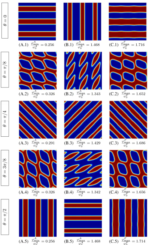
interpret the changes in the micro-texture designs that will be obtained in upcoming examples, they are first considered separately in a series of optimization studies, which are summarized in Figure 3. Here, either the maximization or the minimization of these contributions is carried out while the angle of G for𝜑Aand U for𝜑Fis varied. It is observed that the
minimization of𝜑Adelivers qualitatively similar micro-textures to the maximization of𝜑F. This similarity arises despite
the difference in optimization direction due to the fact that A only contains h3-related terms (see (33)1), whereas F also
contains an h–1-related term (see (37)2). Furthermore, as one might expect, the maximization of𝜑Aleads to micro-textures
that are qualitatively the opposite of those that are obtained from the minimization of𝜑A, in particular with respect to
(A.1) (A.2) (A.3) (A.4) (A.5) (B.1) (B.2) (B.3) (B.4) (B.5) (C.1) (C.2) (C.3) (C.4) (C.5)
FIGURE 3 The objective functions𝜑A
and𝜑Ffrom (58) are employed in
microscopic objective optimization (MicOO) studies: (A) minimization of𝜑A,
(B) maximization of𝜑A, and (C)
maximization of𝜑F. The angle𝜃 (clockwise
from the vertical axis) indicates the direction of G or U (both with unit magnitude).
{h0, hmin, hmax} = {2.2, −0.8, 1.2} was used
in (A,B) and {h0, hmin, hmax} = {2, −1, 1}
the nature of the surface topology as well as its direction. For instance, for an angle of𝜃 = 3𝜋∕8, minimization delivers holes on a surface, whereas maximization delivers bumps, and the direction of these features visually differ by𝜋∕2. In all cases, the minimization or maximization values for𝜑Aand𝜑Fdiffer significantly from the homogeneous surface values
𝜑A
0 =a0‖G‖2and𝜑F0 =e0‖U‖2, which highlight the strong influence of surface texturing.
It is noted that micro-texture designs associated with the minimization of𝜑Fare not displayed because the minimizing
texture is always a homogeneous surface (h = h0). In fact, this may be shown by proving that𝜑F ≥ 𝜑F0. For this purpose,
using (46)2, one may write
𝜑F=U · FU =⟨e⟩‖U‖2+⟨a(ΛTU) · (ΛTU)⟩. (59)
Both contributions are nonnegative and the second one vanishes only for𝚲 = 0, which is only possible for h = h0in the
cell problems of Section 3. To complete the proof, it is therefore sufficient to show that⟨e⟩ ≥ e0. Recalling the definition
(7)2of e as well as h0=⟨h⟩, this requirement is equivalent to ⟨h⟩–1 ≥ ⟨h⟩–1, or⟨h⟩ ≥ ⟨h–1⟩–1. This latter inequality indeed
follows from the fact that the arithmetic average of h > 0 is never less than its harmonic average. Hence, the textured surface can never have a𝜑Fvalue that is less than the one for a homogeneous surface.
7.2.2
Total dissipation
Based on the preceding discussion, it may be stated that the maximization of𝜑 = 𝜑A+𝜑Fis a competition among two
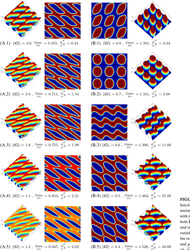
terms, which individually deliver qualitatively opposing micro-textures with respect to surface topology and orientation. On the other hand, the minimization problem is a competition among two terms, one of which always delivers a homo-geneous surface as the optimum. In order to demonstrate how this competition influences the micro-texture design when 𝜑 is the objective function, a MicOO study is carried out where only the magnitude of G is varied (Figure 4). In the case of minimization, when‖G‖ is sufficiently high, 𝜑Adominates𝜑 so that the optimization result is qualitatively closer to
the micro-texture that one would obtain from the direct minimization of𝜑A, compare, for instance, Figure 4(a-1) with
Figure 3(a-2). On the other hand, with decreasing‖G‖, the optimization result approaches toward a homogeneous sur-face because the𝜑Fstarts to dominate the value of𝜑 and the direct minimization of 𝜑Falways delivers a homogeneous
surface. In the maximization study, at large values of‖G‖, 𝜑Aand𝜑Fare of comparable magnitude, although the
optimiza-tion outcome is qualitatively closer to that which would be obtained with𝜑Aalone, compare, for instance, Figure 4(b-1)
with Figure 3(b-2). With decreasing‖G‖, similar to the minimization problem, 𝜑F starts to dominate the value of𝜑
such that the micro-texture design becomes qualitatively similar to that which would be obtained with𝜑Falone,
com-pare, for instance, Figure 4(b-5) with Figure 3(c-2). Note that, in Figure 4(b-1), the holes on the surface are connected, whereas, in Figure 4(b-5), the bumps are connected. Therefore, Figure 4(b-3) represents a transition topology where both are connected.
7.2.3
Interface parameters
In order to assess the influence of various interface parameters on the micro-texture design, a series of MicOO studies will be carried in this section. As demonstrated earlier in Figure 4, maximization of𝜑 = 𝜑A+𝜑Fleads to a very clear
transition between two types of textures, depending on whether𝜑Aor𝜑Fdominates. For this reason, the objective will
be the maximization of𝜑 in the following examples as well.
Figure 5 summarizes the influence of changing h0together with {hmin, hmax}in such a way that the maximum (hmax) and
minimum (hmin) values of h = h0−hremains fixed. The starting value of h0as well as {G, U} are chosen to deliver balanced
values of𝜑Aand𝜑F. Such a parametric change is then observed to only lead to a variation in the area fraction of the features
that are observed in the micro-texture design because⟨h⟩ = h0 changes while {hmin, hmax}remain fixed. The surface
topology does not display stronger changes because the𝜑Aand𝜑Fcontributions remain relatively well balanced. On the
other hand, when h0alone is changed while {hmin, hmax}are held fixed, this corresponds to varying the distance of the
textured surface away from the flat and stationary one. As noted before, A contains only h3-related terms, whereas F also contains an h–1-related term. Therefore,𝜑Fstarts to dominate𝜑 when h
0decreases and a transition in the micro-texture
design is observed, as summarized in Figure 6, similar to the maximization study in Figure 4.
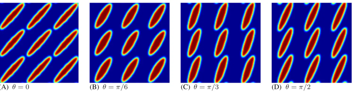
Another similar transition may be observed if the direction of only one vector is varied while all other parameters are held fixed. In Figure 7, the angle associated with U is gradually increased. At all values,𝜑Aand𝜑Fremain well-balanced
so that a strong transition in surface topology is not observed. Nevertheless, the orientation of the design features shift toward a vertical alignment, which, based on the observations of Figure 3, is the one that would be preferred when𝜑F
(A.1) (A.2) (A.3) (A.4) (A.5) (B.1) (B.2) (B.3) (B.4) (B.5)
FIGURE 4 The objective function𝜑 in (58) is (A) minimized or (B) maximized, with𝜃 = 𝜋∕6 as the direction of both U and G.||U|| = 10 is fixed and only the value of||G|| is varied to assess the variation in the relative magnitudes of𝜑A
and𝜑F. In all cases,
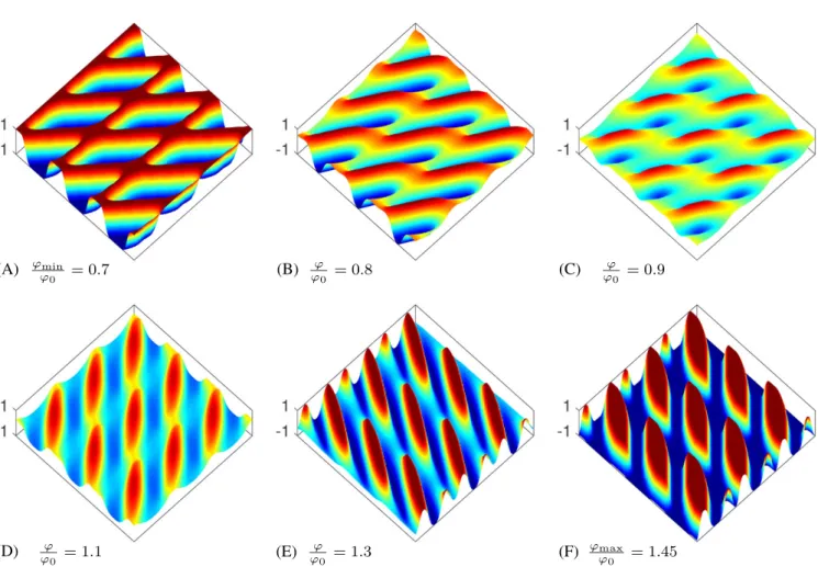
{h0, hmin, hmax} = {2, −1, 1} As noted in Section 6.1, the description of the morphology variable distribution also allows capturing smoothly vary-ing surface geometries in addition to sharper ones. This is demonstrated in Figure 8, where, for a given set of interface parameters,𝜑 is driven to a particular value 𝜑∗, which lies between the maximum and minimum values possible, by
min-imizing a new objective function1
2(𝜑 − 𝜑
∗)2. Near the homogeneous value𝜑
0, the surface topology becomes significantly
smoother and less pronounced, whereas sharper features are obtained for the extremal designs.
Together with the examples that were presented in the previous sections, the examples of this section clearly demon-strate that the optimal surface topology is not necessarily described by simple geometrical features that may enable the use of approximate analytical approaches for both design and homogenization. Consequently, it is advantageous to work in a flexible design space that is offered by homogenization-based topology optimization, which can capture the optimal micro-texture design.
(A) (B) (C) (D)
FIGURE 5 For a fixed angle (𝜃 = 𝜋∕6) for G and U with magnitudes ||G|| = 1 and ||U|| = 10, maximization of 𝜑 = 𝜑A+𝜑Fis carried out
while the value of h0is varied such that h0=2 +𝛿 and {hmin, hmax} = {−1 +𝛿, 1 + 𝛿}, which leads to fixed values of {hmin, hmax} = {1, 3}
(A) (B) (C) (D)
FIGURE 6 For a fixed angle (𝜋∕6) for G and U with magnitudes ||G|| = 1 and ||U|| = 10, maximization of 𝜑 = 𝜑A+𝜑Fis carried out while
the value of h0is varied such that h0=2 −𝛿 and {hmin, hmax} = {−1, 1} are fixed
(A) (B) (C) (D)
FIGURE 7 For a fixed angle (𝜋∕6) for G with magnitude ||G|| = 1, maximization of 𝜑 is carried out while the value angle 𝜃 for U with ||U|| = 10 is varied. Here, {h0, hmin, hmax} = {2.5, −1.5, 0.5}
7.3
Macroscopic objective optimization
For MacOO based on the squeeze-film problem, the influence of the temporal variations in the macroscopic response will be captured by constructing the objective function based on the macroscopic interface dissipation (47) integrated over a cycle, ie, 𝜑 = ∫T Πdt = ∫ T∫ G · AGda dt ⏟⏞⏞⏞⏞⏞⏞⏞⏞⏞⏟⏞⏞⏞⏞⏞⏞⏞⏞⏞⏟ 𝜑A +U · ( || ∫T Fdt ) U ⏟⏞⏞⏞⏞⏞⏞⏞⏞⏞⏞⏞⏟⏞⏞⏞⏞⏞⏞⏞⏞⏞⏞⏞⏟ 𝜑F . (60)
Due to the sinusoidal profile for𝜕h0
𝜕t , it is sufficient to compute the time integral over half a cycle.
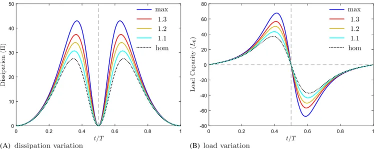
In the classical setup, the second contribution in (60) vanishes because U = 𝟎. For this case, Figure 9 presents a series of micro-textures, which span the range from a maximum dissipation to a homogeneous surface response. The corresponding evolution in the surface topology as well as the change in the macroscopic response of the micro-texture designs are further summarized in Figure 10. Similar to the earlier MicOO study of Figure 8, the flexible optimization framework is able to deliver sharp or smooth topologies depending on the objective function of interest. The macroscopic response is monitored through the dissipation Π from (47) and the load capacity L0 from (55). Although the objective
function is dissipation based, it is observed that a similar ordering for the micro-texture designs is observed for the load capacity as well. In particular, for this problem, the micro-texture that maximizes the dissipation also maximizes the load capacity.
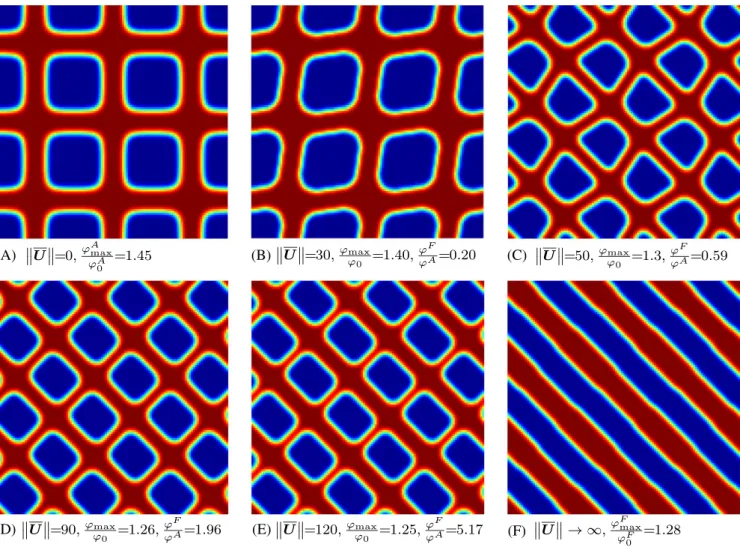
In the modified setup, a tangential velocity U is additionally assigned to+. The orientation of U is fixed to an angle
of𝜋∕4 from the vertical axis, whereas its magnitude is gradually increased. The micro-texture designs that maximize the objective function (60) for each case are presented in Figure 11. These designs start with‖U‖ = 0, which corresponds to the dissipation maximizing result from Figure 9 with𝜑 = 𝜑A, and gradually approach a limit where𝜑Fdominates𝜑 as
‖U‖ increases. In order to highlight this limit more clearly, the micro-texture design that maximizes 𝜑Falone is
addition-ally displayed and indicated with‖U‖ → ∞. Note that the macroscopic response of the micro-texture, as characterized by the flow factor tensors, is isotropic for‖U‖ = 0, whereas it becomes increasingly anisotropic with increasing ‖U‖. The nontrivial variation in the optimal micro-texture design topology during this transition is effectively captured through the homogenization-based topology optimization framework.
(A) (B) (C)
(D) (E) (F)
FIGURE 8 For a fixed angle (𝜋∕6) for G and U with magnitudes ||G|| = 2 and ||U|| = 10, 𝜑∕𝜑0is driven to a value between its maximum and minimum using {h0, hmin, hmax} = {2, −1, 1}
(B)
(A.1) (A.2)
(A.3) (A.4)
FIGURE 9 (A) For the classical squeeze-film problem, the macroscopic objective optimization (MacOO) objective function𝜑 from (60) is first maximized and subsequently also driven to a specified value between the maximum value𝜑maxand the homogeneous surface value𝜑0. Here, {hmin, hmax} = {−0.5, 0.5}. Sample texture profiles along the black lines are compared in (B)
(A) (B)
FIGURE 10 The dissipation and load curves for the micro-textures from Figure 9 are presented. Although the computations are carried out over half a cycle using NT=10 time steps, these curves were generated by computing the macroscopic response of the micro-texture
design over the whole cycle using 100 times steps for a better representation of the temporal variations. The significant deviation from the homogeneous (hom) surface response highlights the influence of the micro-texture
8
M I C RO-T E X T U R E O P T I M A L I T Y
8.1
Global optimality
The optimization framework summarized in Section 6.1 does not guarantee global optimality. Clearly, various ingredients of the numerical setup (eg, topology filtering operation, finite element discretization, optimization stopping criterion)
(A) (B) (C)
(D) (E) (F)
FIGURE 11 For the modified squeeze-film problem with a fixed orientation of U at an angle of𝜋∕4 from the vertical axis, the total dissipation as characterized by the macroscopic objective optimization (MacOO) objective function𝜑 from (60) is maximized for a range of ||U|| values. Here, {hmin, hmax} = {−0.5, 0.5}. Although the limit where 𝜑Fdominates𝜑 is indicated with ||U|| → ∞, this limit is practically
achieved already beyond||U|| = 130
will already influence the degree to which the micro-texture design is optimal. However, apart from this influence, there may be other factors that govern the qualitative or quantitative aspects of optimality such as, respectively, how well the design reproduces the features of the theoretically optimal topology or how close its objective function value is to the theoretical optimum. The purpose of this section is to critically examine the results presented in Section 7 with respect to micro-texture optimality.
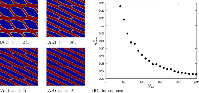
Upon closer examination, Figure 3 reveals that some of the micro-texture designs may be suboptimal. This shortcoming is foremost qualitative in nature. More specifically, the optimal micro-texture has grooves for𝜃 = {0, 𝜋∕4, 𝜋∕2} but not for intermediate angles. One would expect that, if a design with grooves is optimal, then its rotation to an intermediate angle should also be optimal. To highlight this point, the normalized objective function (NOF) value
𝜂 = 𝜑∕𝜑o (61)
that was monitored in these examples will be examined for rotated designs. Now, the NOF value corresponding to the micro-texture design at a given𝜃 that sets the direction for the macroscopic vectors G and U will be indicated by ̃𝜂(𝜃). For all𝜃 values, the homogeneous surface NOF value is 𝜂0 =1. Furthermore, let A(0) and F(0) denote, respectively, the macroscopic flow and stress factor tensors corresponding to a micro-texture design for𝜃 = 0, which has grooves in all three optimization cases of Figure 3. If this design is rotated clockwise through an angle𝛼, the macroscopic response of the rotated design can be characterized through A(𝛼) = QA(0)QTand F(𝛼) = QF(0)QT, where Q(𝛼) is the corresponding
![FIGURE 1 The geometry of the micro-textured lubrication interface [Colour figure can be viewed at wileyonlinelibrary.com]](https://thumb-eu.123doks.com/thumbv2/9libnet/5878310.121262/3.892.72.570.750.1063/figure-geometry-textured-lubrication-interface-colour-figure-wileyonlinelibrary.webp)
![FIGURE 2 The geometry of the micro-textured interface in the unilateral setting [Colour figure can be viewed at wileyonlinelibrary.com]](https://thumb-eu.123doks.com/thumbv2/9libnet/5878310.121262/8.892.317.827.761.1063/figure-geometry-textured-interface-unilateral-setting-colour-wileyonlinelibrary.webp)