Regional model-based computerized ionospheric tomography
using GPS measurements: IONOLAB-CIT
Hakan Tuna1, Orhan Arikan1, and Feza Arikan2
1Department of Electrical and Electronics Engineering, Bilkent University, Ankara, Turkey,2Department of Electrical and
Electronics Engineering, Hacettepe University, Ankara, Turkey
Abstract
Three-dimensional imaging of the electron density distribution in the ionosphere is a crucial task for investigating the ionospheric effects. Dual-frequency Global Positioning System (GPS) satellite signals can be used to estimate the slant total electron content (STEC) along the propagation path between a GPS satellite and ground-based receiver station. However, the estimated GPS-STEC is very sparse and highly nonuniformly distributed for obtaining reliable 3-D electron density distributions derived from the measurements alone. Standard tomographic reconstruction techniques are not accurate or reliable enough to represent the full complexity of variable ionosphere. On the other hand, model-based electron density distributions are produced according to the general trends of ionosphere, and these distributions do not agree with measurements, especially for geomagnetically active hours. In this study, a regional 3-D electron density distribution reconstruction method, namely, IONOLAB-CIT, is proposed to assimilate GPS-STEC into physical ionospheric models. The proposed method is based on an iterative optimization framework that tracks the deviations from the ionospheric model in terms of F2layer critical frequency and maximumionization height resulting from the comparison of International Reference Ionosphere extended to Plasmasphere (IRI-Plas) model-generated STEC and GPS-STEC. The suggested tomography algorithm is applied successfully for the reconstruction of electron density profiles over Turkey, during quiet and disturbed hours of ionosphere using Turkish National Permanent GPS Network.
1. Introduction
Variability in ionospheric electron density (Ne) directly effects the reliability and accuracy of both ground and space-based instrumentation. With increased demands in satellite-based communication and positioning systems, the number of assets that are directly under risk by the variability of space weather and its primary component, Ne, are also on the rise. Computerized ionospheric tomography (CIT) is an effective tool to reconstruct ionospheric electron density values based on satellite measurements. An observable that is used as a “measurement” in CIT is total electron content (TEC), which is formally defined as the line integral of Ne on a given ray path.
Since the advent of satellite-based measurements, various CIT techniques using TEC have been developed in the literature. Very first methods used TEC measurements obtained from low Earth orbit (LEO) satellites for 2-D imaging of the ionosphere along the track of the satellites and the receiver array. Due to the fact that LEO satellites move very fast, ionosphere is considered to be quasi-static during each satellite pass. Using this assumption, Austen et al. [1988] first introduced a method which uses algebraic reconstruction technique (ART) for obtaining a 2-D image of the ionosphere by using TEC data measured between ground receivers and Naval Navigational Satellite System (NNSS) satellites, orbiting the Earth at 1100 km altitude. Since then, iterative reconstruction algorithms became a widely used method in 2-D computerized tomography prob-lems discussed in various studies including but not limited to Raymund et al. [1990], Pryse and Kersley [1992],
Mitchell et al. [1997], and Arikan et al. [2007a]. However, these methods produce a 2-D vertical slice of the
electron density distribution whose location depends on the orbit of the satellites and the receiver locations. Unlike LEO satellites, GPS satellites orbit the Earth at 20,200 km altitude, and therefore, they move very slowly with respect to the ionosphere. This property limits the angle of measurements between a GPS satellite and a receiver station within a time interval in which ionosphere can be considered as quasi-static. On the other hand, GPS system is designed to track at least four satellites at a given time, and ground-based receivers can continuously provide TEC measurements from a number of GPS satellites with varying STEC paths. GPS-based TEC measurements for CIT reconstruction was first introduced in Hajj et al. [1994]. Since then, alternative
RESEARCH ARTICLE
10.1002/2015RS005744
Key Points:
• A novel method for estimating 3-D electron density in the ionosphere is presented
• Ionospheric parameters are optimized by using parametric disturbance surfaces
• Obtained results are compliant with both ionosphere model and measurements
Correspondence to: H. Tuna,
Citation:
Tuna, H., O. Arikan, and F. Arikan (2015), Regional model-based comput-erized ionospheric tomography using GPS measurements: IONOLAB-CIT,
Radio Sci., 50, 1062–1075,
doi:10.1002/2015RS005744.
Received 15 MAY 2015 Accepted 16 SEP 2015
Accepted article online 19 SEP 2015 Published online 24 OCT 2015
©2015. American Geophysical Union. All Rights Reserved.
ionospheric tomography techniques employing GPS-TEC measurements have been developed making use of increasing number of local and global GPS receiver networks. However, due to the complicated geometry of data acquisition, most of the developed tomographic reconstruction techniques have to be custom tailored to the application or to the network.
The sparsity of GPS-based measurements becomes even more challenging when the goal is reconstruction of 3-D electron density. The increased number of unknowns in 3-D geometry complicates the solution signif-icantly, and this would render the reconstruction problem next to impossible to solve, if no prior information on the electron density distribution is introduced. Therefore, to overcome the issues of insufficient data, many methods use some kind of regularization together with a background ionosphere model such as those dis-cussed in Fridman et al. [2006] and Yao et al. [2014]. Some CIT methods utilize basis functions for constraining the solution in a predetermined problem space as given in Arikan et al. [2007b] and Erturk et al. [2009]. Exam-ples of model-free iterative approaches can be found in Lee et al. [2008] and Wen et al. [2008]. CIT using neural networks is also proposed in the literature as given in Ma et al. [2005]. Comprehensive reviews of general ionospheric tomography methods are provided in Kunitsyn and Tereshchenko [2003] and Bust and Mitchell [2008].
Since TEC measurements available for 3-D ionospheric reconstruction are not dense enough, reconstruction techniques based on only TEC measurements demand new regularization techniques or declaration of some cost functions for minimization. Yet, in this case, the solution set may include physically unreliable or inac-curate results. Because of the sparsity of the measurements, the prior information about the problem has a great importance. The reconstruction methods, which do not depend on any ionospheric models or take into account any physical properties of the ionosphere, produce same results for given measurement set, regardless of the location of the measurements or time. Thus, it is of utmost importance to utilize a physically acceptable model in solution of ill-determined ionospheric tomography problems.
One of the most commonly used ionospheric models is International Reference Ionosphere (IRI) [Bilitza et al., 2014]. Since the 90 km to 2000 km height range of IRI model is not sufficient to represent the structure of ionosphere and plasmasphere up to GPS orbital radius, IRI Extended to Plasmasphere (IRI-Plas) [Gulyaeva and
Bilitza, 2012] is used in this study.
In this study, a novel method for obtaining robust, high-resolution regional 3-D electron density distribu-tion in the ionosphere by assimilating available GPS-TEC measurements into the IRI-Plas model is presented. IONOLAB-CIT does not use any regularization method or basis functions, but instead, it adapts the physi-cal parameters used in the IRI-Plas model to provide physiphysi-cally adaptive reconstructions that provide better agreement with the available GPS-TEC measurements. The default ionospheric parameters used in IRI-Plas model (namely, the F2layer critical frequency, f0F2, and maximum ionization height, hmF2) are adjusted using a parametric perturbation surface over the region of interest. The parameters of the perturbation surface are optimized such that the resultant 3-D electron density distribution is in compliance with the STEC estimates obtained from a GPS satellite-receiver network in the region. In development of the proposed CIT method, quadratic parametric perturbation surfaces for both f0F2and hmF2are utilized [Arikan et al., 2012; Tuna et al.,
2013]. It is observed that the quadratic perturbation surfaces produce higher errors at regional borders due to insufficient number of GPS network receivers. A simple approach utilizing a planar perturbation surface only on the f0F2parameter is given in Tuna et al. [2014b]. In this study, the perturbation surfaces are chosen as
planar, which reduces the reconstruction error at the region borders. Also, in this study, instead of bound-ing the perturbation surfaces, perturbed critical frequency and maximum ionization height surfaces are bounded using a mathematical function that models the physical behavior of ionosphere for a midlatitude region. In order to decrease the computational cost of the proposed method, precomputed electron den-sity matrices are used for model-based STEC calculation. The perturbation surface parameters are optimized by using numerical optimization methods: gradient descent algorithm, Broyden-Fletcher-Goldfarb-Shanno (BFGS) algorithm [Broyden, 1970; Fletcher, 1970; Goldfarb, 1970; Shanno, 1970], and particle swarm optimiza-tion (PSO) [Kennedy and Eberhart, 1995]. The reduced number of optimizaoptimiza-tion parameters due to the planar perturbation surfaces, using precomputed electron density voxel values for model-based STEC calculation and the use of bounding functions for modeling the physical limits of ionosphere parameters in this study, not only provides faster convergence and reduces the computational complexity but also increases the reliability and accuracy of the reconstruction.
IONOLAB-CIT is applied to reconstruct regional 3-D ionosphere over Turkey, using the Turkish National Per-manent GPS Network (TNPGN) for both geomagnetically calm and storm days of ionosphere. The map of the GPS receivers can be accessed via http://www.tkgm.gov.tr/tr/icerik/tusaga-aktif-0. IONOLAB-STEC method [Arikan et al., 2003; Nayir et al., 2007; Arikan et al., 2008] is used for obtaining GPS-STEC measurements. It is observed that the proposed method provides highly reliable and accurate reconstructions of 3-D ionospheric electron density profiles where IRI-Plas-STEC and GPS-STEC are in good agreement even in the geomagnetic storm hours.
In section 2, the data sets of measurement-based STEC and model-based STEC that are used in the CIT algorithm are introduced. In section 3, the proposed novel, regional CIT algorithm, IONOLAB-CIT is briefly discussed. The performance of the CIT algorithm using synthetic ionosphere and the real world examples of reconstructions for calm and storm days for a GPS network are provided in section 4. Remarks and conclusions are given in section 5.
2. Preparation of Data Sets
In situ measurements of electron density distribution in the ionosphere is not practical to provide enough spatial coverage for even regional 3-D ionospheric imaging. Therefore, remote sensing techniques are used to obtain information about electron density distribution over the region of interest. Total electron content (TEC) is one of the basic observables of ionosphere. The total number of electrons on a slant path between the satellite and the receiver is called slant TEC (STEC). STEC corresponds to the total number of electrons on a ray path between the satellite and the receiver with a cross section area of 1 m2. It is expressed in terms of
TEC unit (TECU), which is equal to 1016electrons/m2. The proposed tomography algorithm is based on the
comparison of measurement-based STEC and model-based STEC. In this section, the preparation of these data sets is briefly discussed.
2.1. Measurement-Based STEC: IONOLAB-STEC
In recent years, the most common method of TEC estimation is based on the dual-frequency ground-based Global Positioning System (GPS) receiver recordings of pseudorange and phase delay. There are various tech-niques used for estimating STEC in the ionosphere, such as those in Mo et al. [1997], Kersley et al. [2004], Garner
et al. [2010], and Nayir et al. [2007]. GPS-STEC values can be estimated using IONOLAB-STEC method
includ-ing differential receiver bias as IONOLAB-BIAS as discussed in detail in various publications includinclud-ing Nayir
et al. [2007] and Arikan et al. [2003, 2008]. The computation of IONOLAB-TEC is provided as a space weather
service at www.ionolab.org and the details are provided in Sezen et al. [2013a]. In this study, IONOLAB-STEC method is used in preparation of measurement-based STEC values, providing highly reliable, accurate, and robust GPS-STEC estimates with 30 s time resolution.
2.2. Model-Based STEC: IRI-Plas-STEC
International Reference Ionosphere (IRI) is one of the most acknowledged climatic models of ionosphere [Bilitza et al., 2014]. For any given location and time, IRI computes monthly medians of electron density, electron temperature, ion temperature, and ion composition in the altitude range from 50 km to 2000 km. International Reference Ionosphere Extended to Plasmasphere (IRI-Plas) is a recent version of IRI that enables assimilation of TEC, F2layer critical frequency and maximum ionization height in computation of electron
density up to the GPS orbital height of 20,000 km [Gulyaeva and Bilitza, 2012; Gulyaeva et al., 2011].
In this study, the underlying ionospheric model is chosen to be IRI-Plas, available at http://ftp.izmiran.ru/ pub/izmiran/SPIM/. The model-based STEC is computed from IRI-Plas as IRI-Plas-STEC as discussed in detail in Tuna et al. [2014a]. IRI-Plas-STEC is provided online as a space weather service at www.ionolab.org. It is observed that IRI-Plas-STEC is in very good agreement with IONOLAB-STEC for the calm days of iono-sphere, even without the assimilation of TEC into IRI-Plas. For the storm days, if TEC values are not input into the model, then the difference between IRI-Plas-STEC and IONOLAB-STEC increases significantly. Also, on stormy days, measurement-based STEC values suffer from discontinuities and disruptions [Arikan et al., 2014;
Shukurov et al., 2014].
In the IRI-Plas-STEC computation, STEC value on a slant path s, between a receiver-satellite pair, is estimated by integrating the electron density as a nonuniform Riemann sum over voxels that are traced on path s [Tuna et al., 2014a]. In order to reduce the computational cost required for calculation of STEC values for all receiver-satellite pairs in a GPS receiver network, electron density in each voxel can be computed using IRI-Plas
and stored in a database. Thus, for each time frame, IRI-Plas-STEC values between the GPS network receivers and the satellites can be expressed as an inner product of two vectors:
Ts= Bs⋅ N, (1)
where N is the vectorized electron density values for all voxels in the region of interest and Bsis the vector of precalculated values for the corresponding receiver-satellite geometry of the slant path s. Appropriate spatial resolution for the voxels can be chosen as 1∘ in both latitude and longitude. Three-dimensional voxels are stacked in altitude increments starting from a height of 100 km up to 20,000 km. The altitude increments of the voxels are chosen to be 1 km in between 100 km and 600 km, 10 km in between 600 km and 1300 km, and 50 km in between 1300 km and 20,000 km. These altitude increments are obtained by modifying the original IRI-Plas code for higher-altitude resolution.
3. Regional CIT Using IRI-Plas and IONOLAB-STEC: IONOLAB-CIT
Proposed 3-D electron density estimation model employs fusion of real measurements obtained from a GPS satellite-receiver network and IRI-Plas model together. The input parameters of IRI-Plas model in the region of interest are optimized such that the resultant 3-D electron density profile obtained from IRI-Plas model is in compliance with the real GPS-TEC measurements. In this study, the ionospheric parameters to be optimized are selected as the critical frequency of the F2layer which has the highest electron density in the ionosphere
and the maximum ionization height. They are denoted with f0F2and hmF2, respectively, and they are two
important parameters affecting the total electron content in the ionosphere.
It is possible to obtain a physically admissible set of model-based VTEC values from IRI-Plas model by changing its inputs f0F2and hmF2parameters at a location of interest [Sezen et al., 2013b]. However, in order to fit 3-D
electron density profile obtained from IRI-Plas model to a large set of STEC measurements obtained in a region, the spatial properties of f0F2and hmF2have to be considered. Along with many other ionospheric parameters,
the values of f0F2and hmF2are spatially smooth functions. Spatial variations of f0F2and hmF2over the region of
interest are modeled as superposition of planar perturbation surfaces and the default f0F2and hmF2surfaces generated by the IRI-Plas model.
The latitude and longitude interval of region of interest over which 3-D reconstruction of the ionospheric electron density should be obtained can be defined as
A = {(𝜙, 𝜆)|𝜙min≤ 𝜙 ≤ 𝜙max, 𝜆min≤ 𝜆 ≤ 𝜆max}, (2) where𝜙 and 𝜆 are geodetic latitude and longitude, respectively. The planar perturbation surfaces on the default f0F2and hmF2values in region A are denoted with EFand EH, respectively. In order to compute the perturbation surface parameters in a geometry-free environment, the perturbation surfaces are modeled in normalized coordinates bounded within [−1, 1] interval. The normalized coordinates can be calculated as
𝜙n= 2𝜙 − 𝜙max−𝜙min 𝜙max−𝜙min , (3) 𝜆n= 2𝜆 − 𝜆max−𝜆min 𝜆max−𝜆min . (4)
The planar perturbation surfaces EF and EH in region A can be represented by three parameters each, contained in vector m:
m =[mf, mh], (5)
where mfand mhare defined as
mf=[mf1, mf2, mf3], (6) mh=[mh 1, m h 2, m h 3 ] . (7)
The values of the planar perturbation surfaces EFand EHat any location in A can be calculated by using the following equations:
EF(𝜙, 𝜆, mf) = mf1𝜙n+ mf2𝜆n+ mf3, (8)
EH(𝜙, 𝜆, mh) = mh1𝜙n+ mh2𝜆n+ mh3. (9)
Specifically, perturbed f0F2and hmF2values for any given location in A are obtained by using the following equations: Fopt(𝜙, 𝜆, mf) = S ( F(𝜙, 𝜆) + EF(𝜙, 𝜆, mf), Fmin, Fmax ) , (10) Hopt(𝜙, 𝜆, mh) = S ( H(𝜙, 𝜆) + EH(𝜙, 𝜆, mh), Hmin, Hmax ) , (11)
where F(𝜙, 𝜆) and H(𝜙, 𝜆) are the default values for f0F2and hmF2obtained from IRI-Plas for given latitude𝜙
and longitude𝜆, Fopt(𝜙, 𝜆, mf) and Hopt(𝜙, 𝜆, mh) are the modified IRI-Plas input parameters for fitting the 3-D
electron density profile to measurements by using the perturbation surface parameters in mfand mh, and S is a sigmoid-like function for bounding the results within given physical limits, Fmin− Fmaxand Hmin− Hmax.
Sis defined in a way that if the input value is in between and not close to the bounding limits, it returns the same value for the output. However, if the input value is close to the bounding limits, or exceeds these limits,
Sprovides an output within the set limits. Assume that, the limits of S are𝜎1for the lower limit, and𝜎2for the higher limit. The one-to-one function S is defined as
S(r, 𝜎1, 𝜎2) = ⎧ ⎪ ⎨ ⎪ ⎩ 𝜎1+ 2(𝜎′ 1−𝜎1) 1+e−2𝜇1 if r< 𝜎1′ r if𝜎′ 2≥ r ≥ 𝜎 ′ 1 𝜎2+ 2(𝜎′ 2−𝜎2) 1+e−2𝜇2 if r> 𝜎2′ , (12) where𝜎′ 1,𝜎′2,𝜇1, and𝜇2are 𝜎′ 1=𝜎1+ 𝜎2−𝜎1 10 , (13) 𝜎′ 2=𝜎2− 𝜎2−𝜎1 10 . (14) 𝜇1= r −𝜎′ 1 𝜎′ 1−𝜎1 , (15) 𝜇2= r −𝜎′ 2 𝜎′ 2−𝜎2 . (16)
A physically admissible 3-D ionospheric reconstruction can be obtained for any choice of parameters in m. The challenge is the identification of the optimal m for which the synthetically generated 3-D ionosphere would provide STEC values that are closest to the actual measurements. Furthermore, the physical relation between the ionosphere parameters obtained for given m should also be considered. For a specific choice of m, the following cost function can be used in the search of optimal m:
C(m) = √ √ √ √∑s ( Ts(m) − Ms)2 ∑ sM2s +𝜌 √ √ √ √∑i ∑ j ( Hopt(𝜙i, 𝜆j, mh) − H def(𝜙i, 𝜆j, mf) )2 ∑ i ∑ jHdef(𝜙i, 𝜆j, mf)2 , (17)
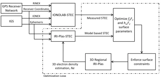
Figure 1. Graphical structure of the proposed 3-D ionospheric reconstruction technique. Input parameters that are
searched by numerical optimization methods are fed to regional IRI-Plas model so that the discrepancy between synthetic STEC values derived from the model-based reconstruction and the actual STEC values derived from the GPS measurements is minimized.
where Ts(m) is the calculated STEC value along s from the 3-D electron density matrix obtained from IRI-Plas in region A for the given parameter set m; Msis the real GPS-TEC measurement obtained along s by using GPS systems; Hdef(𝜙i, 𝜆j, mf) is the default hmF2value obtained from IRI-Plas model for given latitude, longitude,
and Fopt(𝜙i, 𝜆j, mf) values;𝜙iand𝜆jare discrete latitude and longitude values spanning the region A with 1∘ step sizes; and𝜌 is an adjustable weight parameter which determines the relaxation on the physical relation between f0F2and hmF2parameters.
In order to find the m which minimizes C(m), gradient descent algorithm, BFGS algorithm, and PSO method are utilized. The gradient descent is an iterative optimization technique which uses the first order derivatives of the function for taking steps in the problem space, whereas BFGS method uses both the first and second order derivatives of the function. In order to prevent narrow valleys in the problem space, which causes pathological problems in both methods, and since the effect of hmF2parameter on the STEC values is very low with respect
to f0F2parameter, the optimization parameters are selected as follows:
m′= [m
f, 100mh] (18)
The starting point in both methods is set to origin in 6-D problem space, which corresponds to the default IRI-Plas solution. The initial step size at each iteration is selected as an exponentially decaying function with respect to iteration number and does not depend on the gradient. A backtracking line search based on Armijo-Goldstein condition [Armijo, 1966] is employed in both methods, with a step size reduction ratio of 1/2.
Figure 2. Cost function for three different optimization methods with respect to iteration count, obtained for synthetic
measurement data on 1 June 2011, 10:00 GMT. The cost value obtained by using default IRI-Plas parameters is 0.195. Solid line shows cost function obtained by gradient descent algorithm, dashed line shows the cost function obtained by BFGS method, and the line with circle markers shows cost function obtained by PSO.
Figure 3. 1 September 2011, 12:00 GMT. (a) Cost function for three different optimization methods with respect to
iteration count, (b) IRI-Plas TEC (TECU), (c) IONOLAB-CIT TEC (TECU), (d) optimizedf0F2perturbation surface (MHz), and (e) optimizedhmF2perturbation surface (km).
Both gradient descent and BFGS methods fail when optimizing functions with local minima. In this CIT problem, it is not possible to determine if the problem space has local minima or not, since the problem space depends on the real measurements obtained from GPS receivers. For this reason, PSO, which is a stochastic and iterative optimization technique, is also employed. It uses a swarm of candidate solution points, called particles, and tries to find the optimum solution by simply moving the particles in the problem space. Particles have the memory of the best position they have found so far and communicate with each other to learn the
Figure 4. 10 March 2011, 12:00 GMT. (a) Cost function for three different optimization methods with respect to iteration
count, (b) IRI-Plas TEC (TECU), (c) IONOLAB-CIT TEC (TECU), (d) optimizedf0F2perturbation surface (MHz), and (e) optimizedhmF2perturbation surface (km).
best position swarm has found so far. At each iteration, particles move in the problem space based on their velocity and acceleration parameters. The updated locations of the particles are evaluated by using the cost function. The particles update their best personal positions based on the results, and they communicate with each other for updating the global best position of the swarm. After that, particles are accelerated toward the best personal solution and the best global solution, with random amounts. PSO does not make assumptions about the problem space, and it is highly robust against functions with local minima. In this paper, global communication topology is used in PSO, in which every particle except the particle itself contributes to the
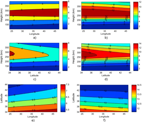
Figure 5. Electron density slices obtained by using IONOLAB-CIT for both storm and calm days, in terms of 1011
electrons/m3. (a), (c), and (e) Results for 1 September 2011, 12:00 GMT, for fixed latitude (39∘N), fixed longitude (34∘E), and fixed height (250 km), respectively. (b), (d), and (f ) Results for 10 March 2011, 12:00 GMT, for fixed latitude (39∘N), fixed longitude (34∘E), and fixed height (250 km) respectively.
calculation of the global best position of that particle. The particle velocity and particle positions are updated by using the following equations.
Vn k = w1Vk−1n + w2Z1(Bnk− P n k) + w3Z2(Dnk− P n k), (19) Pnk+1= Pnk+ Vkn. (20) where Pn
kis the position of the particle n at iteration k, V n
kis the velocity of the particle n at iteration k, B n kis the personal best position of particle n at iteration k, and Dn
kis the global best position of particle n at iteration k.
Z1and Z2are random variables uniformly distributed in [0, 1]. The velocity update coefficient w1is selected as 0.5, the acceleration coefficients w2and w3are selected as 0.05, and the number of particles in the simulations are selected as 100, as they are used in Tuna et al. [2013].
IONOLAB-CIT method produces a 3-D electron density distribution for the given TEC measurement set by using parameter optimization methods and IRI-Plas ionosphere model. The structure of the IONOLAB-CIT is shown in Figure 1.
4. Results
This section contains experimental results obtained by IONOLAB-CIT method. In the following results, the region of interest is chosen over Turkish borders. The limits of the region for estimating the 3-D electron
Figure 6. Electron density values along the GPS receiver-satellite path, obtained from IRI-Plas model and reconstructed
3-D electron density distributions. (a) 1 September 2011, 12:00 GMT, receiver station: “anrk” (39.9∘N, 32.8∘E), GPS satellite no.: 25 (73.7∘elevation,−25.3∘azimuth), (b) 1 September 2011, 12:00 GMT, receiver station: “boyt” (41.5∘N, 34.8∘E), GPS satellite no.: 12 (69.6∘elevation, 92.3∘azimuth), (c) 10 March 2011, 12:00 GMT, receiver station: “anrk” (39.9∘N, 32.8∘E), GPS satellite no.: 23 (73.3∘elevation,−25.0∘azimuth), and (d) 10 March 2011, 12:00 GMT, receiver station: “mrsi” (36.8∘N, 34.6∘E), GPS satellite no.: 20 (76.1∘elevation, 83.0∘azimuth).
density distribution is selected in between 34∘ and 44∘ latitude, 24∘ and 47∘ longitude, and 100 and 20,000 km in height. Five different approaches are conducted in the experiments.
First, in order to validate the proposed ionospheric tomography method, its performance is experimented on the simulated data. Parametric disturbance surfaces over default IRI-Plas parameters f0F2and hmF2are
con-structed with parameters m = [0.8, −0.4, 0.5, 12, 8, 15]. Then, a 3-D electron density distribution is obtained
Table 1. Cost Function Obtained After 100 Iterations for Each Method for Various Dates
Date Ionospheric Weather IRI-Plas GD BFGS PSO
21.03.2011, 10:30 GMT Calm 0.1486 0.0733 0.0731 0.0738 21.03.2011, 23:00 GMT Calm 0.1490 0.0786 0.0786 0.0810 12.06.2011, 06:15 GMT Calm 0.2190 0.0414 0.0414 0.0470 12.06.2011, 17:45 GMT Calm 0.0592 0.0482 0.0482 0.0505 21.09.2011, 03:30 GMT Calm 0.1558 0.0836 0.0835 0.1021 21.09.2011, 13:45 GMT Calm 0.1803 0.0495 0.0491 0.0528 25.12.2011, 06:00 GMT Calm 0.1058 0.0593 0.0593 0.0615 25.12.2011, 16:30 GMT Calm 0.1800 0.1641 0.1641 0.1645 05.02.2011, 01:00 GMT Storm 0.2299 0.1012 0.0952 0.1095 28.05.2011, 12:15 GMT Storm 0.3014 0.0340 0.0339 0.0364 06.08.2011, 00:30 GMT Storm 0.1199 0.0838 0.0683 0.0887 01.11.2011, 15:30 GMT Storm 0.3636 0.1577 0.1572 0.1583
Table 2. Comparison of Measured STEC Values, STEC Values Calculated from IRI-Plas Model and Predicted STEC Values Calculated from Optimized 3-D Electron
Density Distributions for 10 March 2011, 12:00 GMT
Receiver Station Receiver Location GPS Satellite Number Elevation Angle Azimuth Angle Measured STEC IRI-Plas STEC Predicted STEC
Ankara, anrk 39.9N∘, 32.8E∘ 20 76∘ 90∘ 43.10 24.47 43.04
Ankara, anrk 39.9N∘, 32.8E∘ 23 73∘ −33∘ 45.87 24.65 43.62
Ankara, anrk 39.9N∘, 32.8E∘ 32 47∘ 102∘ 57.46 30.39 53.31
Malatya, maly 38.3N∘, 38.2E∘ 13 44∘ −83∘ 55.78 32.74 57.39
Malatya, maly 38.3N∘, 38.2E∘ 20 81∘ 82∘ 41.76 24.53 42.50
Malatya, maly 38.3N∘, 38.2E∘ 23 69∘ −39∘ 44.65 25.33 44.45
by using IRI-Plas model and disturbed f0F2and hmF2parameter surfaces, for time 1 June 2011, 10:00 GMT. By
using the actual geometry of TNPGN receivers and GPS satellites at that time, synthetic STEC measurements are calculated by using the method described in Tuna et al. [2014a]. Cost function with respect to iteration number obtained for each optimization method is given in Figure 2, where𝜌 is used as 0 in the cost function. The initial cost function obtained for the synthetically disturbed ionosphere is 0.195, and all methods have successfully decreased the cost function below 0.020 after 100 iterations. However, results show that BFGS is the fastest converging result among all proposed methods.
Second, the proposed method is experimented on the real measurement data (IONOLAB-STEC) which has been obtained from Turkish National Permanent GPS Network (TNPGN) stations. A solar calm day (1 September 2011, at 12:00 GMT), and a solar storm day (10 March 2011, at 12:00 GMT) is used in sim-ulations. The storm lists are obtained from http://www.izmiran.ru/ionosphere/weather/storm/. In order to choose the appropriate set of STEC measurements from IONOLAB-STEC database obtained from TNPGN sta-tions, all receiver stations are checked if they have valid STEC measurements with any satellites for the given time. Next, STEC measurements for elevation angles which are lower than 30∘ are filtered out. Since 80% of the electron density distribution in the ionosphere is in between 100 km and 1500 km height, the STEC measurements measured along slant paths which stay inside the region A below 1500 km elevation are selected as valid measurements to be used in the proposed ionospheric reconstruction technique. In this part of the experiment,𝜌 is selected as 0.1. Results obtained for the selected days are given in Figures 3 and 4, respectively. Figures 3a and 4a show the cost value as a function of iteration number for each optimization method. As seen from these figures, the cost is decreased from 0.16 to 0.07 for the quiet day and from 0.43 to 0.03 for the disturbed day, respectively. Figures 3b and 4b show the default VTEC maps obtained by using IRI-Plas model in the region. Figures 3c and 4c show the VTEC maps calculated by using IRI-Plas model and the optimized parameters obtained by BFGS method. Figures 3d and 3e and 4d and 4e show the perturba-tion surfaces corresponding to the optimized parameters obtained by BFGS method. Results show that the required number of iterations for convergence of the obtained reconstructions for both the quiet and the disturbed days are very similar. Figure 5 and 6 presents various visualizations of the obtained results from the proposed CIT technique. Figure 5 shows electron density slices extracted from 3-D electron density dis-tributions obtained by IONOLAB-CIT method with BFGS optimization for both days. In Figures 5a and 5b, the electron density values along latitude 39∘N is shown with respect to longitude and height. In Figures 5c and 5d, the electron density values along longitude 34∘E is shown with respect to latitude and height. In Figures 5e
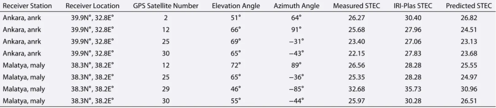
Table 3. Comparison of Measured STEC Values, STEC Values Calculated from IRI-Plas Model and Predicted STEC Values Calculated from Optimized 3-D Electron
Density Distributions for 1 September 2011, 12:00 GMT
Receiver Station Receiver Location GPS Satellite Number Elevation Angle Azimuth Angle Measured STEC IRI-Plas STEC Predicted STEC
Ankara, anrk 39.9N∘, 32.8E∘ 2 51∘ 64∘ 26.27 30.40 26.82
Ankara, anrk 39.9N∘, 32.8E∘ 12 66∘ 91∘ 25.68 27.96 24.51
Ankara, anrk 39.9N∘, 32.8E∘ 25 69∘ −31∘ 23.40 27.06 23.13
Ankara, anrk 39.9N∘, 32.8E∘ 30 65∘ −43∘ 22.15 27.83 23.68
Malatya, maly 38.3N∘, 38.2E∘ 12 72∘ 89∘ 26.56 28.28 25.55
Malatya, maly 38.3N∘, 38.2E∘ 25 65∘ −36∘ 25.35 28.28 24.97
Malatya, maly 38.3N∘, 38.2E∘ 29 46∘ −85∘ 32.68 35.73 30.96
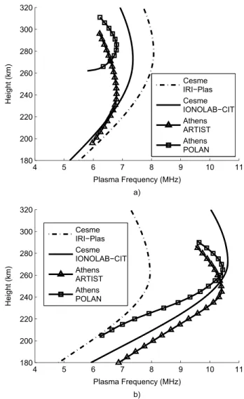
Figure 7. Comparison of plasma frequencies obtained by using IRI-Plas model and proposed IONOLAB-CIT technique at
Çe¸sme (38.3∘N, 26.4∘E), with the plasma frequencies obtained by using ionosonde measurements and two automatic ionogram scaling techniques ARTIST and POLAN, at Athens (38.0∘N, 23.5∘E), on a) calm day (1 September 2011, 12:00 GMT), b) storm day (10 March 2011, 12:00 GMT).
and 5f, the electron density values at 250 km height is shown with respect to latitude and longitude. Figure 6 shows the comparison of electron density values along sample GPS receiver-satellite paths computed from 3-D electron density distributions of IRI-Plas model and proposed CIT technique.
Third, the second experiment is repeated on the real measurement data (IONOLAB-STEC) for different dates and ionospheric weather, and the performance of each optimization method are listed in Table 1. Results show that the performance of three methods is very similar in most scenarios. However, in all cases, BFGS outperforms other two. Small values for cost functions obtained after using optimization methods can be explained as noise in the TEC measurements. If the cost function is very high that it cannot be explained by the measurement errors, this may indicate the necessity to use a higher order parametric perturbation surface or failure of the ionosphere model to model the ionospheric electron density adequately for that case. Fourth, to investigate reliability of the reconstructions, the data obtained at two GPS stations located in Ankara and Malatya are excluded from the measurement set input to the reconstruction algorithm. The proposed CIT method run with the remaining STEC measurements for 2 days used in the second part of the experiments, by using the BFGS optimization technique. Then the missing STEC measurements at the two left out stations are computed from the reconstructions and compared with the actual STEC measurements corresponding to these stations. Tables 2 and 3 show comparison of measured and reconstructed STEC values. The results show that the proposed CIT technique provides reliable reconstructions.
Fifth, to provide further verification on the performance of the proposed IONOLAB-CIT technique, ionosonde measurements of Athens station (38.0∘N, 23.5∘E) are compared to the IONOLAB-CIT results over Çe¸sme, ˙Izmir (38.3∘N, 26.4∘E), which is approximately 225 km away from the Athens ionosonde. Figures 7a and 7b show comparison of plasma frequencies with respect to height provided by IRI-Plas model and IONOLAB-CIT technique, with the plasma frequencies obtained by using ionosonde measurements and two widely used automatic ionogram scaling techniques ARTIST [Huang and Reinisch, 1996] and POLAN [Titheridge, 1985], for calm and storm days, respectively. BFGS optimization technique is used in both IONOLAB-CIT results. The ionosonde measurement data is obtained from http://ngdc.noaa.gov/ionosonde/data/. Results show that the proposed method provides closer results to the ionosonde measurements with respect to IRI-Plas model. The proposed CIT method conducts a search for the optimal parameters by using iterative optimization approaches. Among the experimented three different optimization methods, gradient descent and BFGS are deterministic methods for given starting point and step size parameters. PSO, on the other hand, is a stochastic optimization method, and the results obtained for different runs typically differ from each other. The computa-tional cost of the PSO technique is higher than the other two approaches. However, since the computation of cost functions for each particle in PSO algorithm can be performed independently, the PSO technique is very suitable for parallel computation. If the computational cost is not an issue, PSO technique can be preferred for its robustness against local minima, by using higher number of particles and iterations. Other than this, BFGS method is shown to be the optimum choice between three for optimization of ionospheric parameters.
5. Conclusion
A new approach for estimation of 3-D electron density profile in the ionosphere by using both the fusion of GPS-TEC measurements and IRI-Plas model is presented. Three-dimensional electron density obtained from IRI-Plas model is adjusted by using IRI-Plas input parameters over Turkey in a way that synthetic measure-ments calculated from the 3-D electron density profile is in compliance with real GPS-TEC measuremeasure-ments. IRI-Plas input parameters over Turkey are represented with additive parametric perturbation surfaces. The surface parameters are optimized by using gradient descent, BFGS and PSO methods. By using actual GPS measurement data obtained from IONOLAB-STEC, experiments using the f0F2and hmF2as the optimization parameters over Turkey are presented. Results show that the reconstructed 3-D electron density profiles have significantly improved conformity with the measurements, with respect to the default 3-D electron density profiles obtained from IRI-Plas model. Reconstructions are also validated by predicting the STEC mea-surements missing in the input STEC measurement set successfully. Obtained results are compared with ionosonde measurements in Athens, and it is shown that the proposed method is in better agreement with the ionosonde measurements with respect to IRI-Plas model. The proposed approach can easily be extended to operate over a larger set of parameters if necessary. Ionospheric measurements like ionosonde measure-ments, GPS occultation measurements can be added to the proposed method by modifying the cost function accordingly.
References
Arikan, F., C. B. Erol, and O. Arikan (2003), Regularized estimation of vertical total electron content from Global Positioning System data,
J. Geophys. Res., 108(A12), 1469, doi:10.1029/2002JA009605.
Arikan, F., H. Nayir, U. Sezen, and O. Arikan (2008), Estimation of single station interfrequency receiver bias using GPS-TEC, Radio Sci., 43, RS4004, doi:10.1029/2007RS003785.
Arikan, F., U. Sezen, T. L. Gulyaeva, and O. Cilibas (2014), Online, automatic, ionospheric maps: IRI-PLAS-MAP, Adv. Space Res., 55(8), 2106–2113, doi:10.1016/j.asr.2014.10.016.
Arikan, O., F. Arikan, and C. B. Erol (2007a), 3-D Computerized ionospheric tomography with random field priors, in Mathematical Methods in
Engineering, pp. 325–334, Springer, Netherlands., doi:10.1007/978-1-4020-5678-9_28
Arikan, O., F. Arikan, and C. B. Erol (2007b), Computerized ionospheric tomography with the IRI model, Adv. Space Res., 5, 859–866, doi:10.1016/j.asr.2007.02.078.
Arikan, O., H. Tuna, F. Arikan, and T. L. Gulyaeva (2012), Reconstruction of 3-D ionospheric electron density distribution by using GPS measurements and IRI-Plas model, AOGS-AGU (WPGM) Joint Assembly 2012, Singapore, 13-17 August.
Armijo, L. (1966), Minimization of functions having Lipschitz continuous first partial derivatives, Pacific J. Math., 16(1), 1–3, doi:10.2140/pjm.1966.16.1.
Austen, J. R., S. J. Franke, and C. H. Liu (1988), Ionospheric imaging using computerized tomography, Radio Sci., 23(3), 299–307, doi:10.1029/RS023i003p00299.
Bilitza, D., D. Altadill, Y. Zhang, C. Mertens, V. Truhlik, P. Richards, L. A. McKinnell, and B. Reinisch (2014), The International Reference Ionosphere 2012—A model of international collaboration, J. Space Weather Space Clim., 4, A07, doi:10.1051/swsc/2014004.
Broyden, C. G. (1970), The convergence of a class of double-rank minimization algorithms 1. General considerations, J. Inst. Math. Appl., 6(1), 76–90, doi:10.1093/imamat/6.1.76.
Acknowledgments
TNPGN RINEX data set is made available to IONOLAB group for TUBITAK109E055 project at http://www.ionolab.org/. This data set can be accessed by the per-mission from TUBITAK and General Command of Mapping of Turkish Army (http://www.hgk.msb.gov.tr/). This study is supported by the joint TUBITAK112E568 and RFBR13-02-91370-CTa and joint TUBITAK114E092 and ASCR 14/001 projects. The ionospheric storm lists are provided by http://www.izmiran.ru/ionosphere/ weather/storm/. The ionosonde measurement data are obtained from http://ngdc.noaa.gov/ionosonde/data/.
Bust, G. S., and C. N. Mitchell (2008), History, current state, and future directions of ionospheric imaging, Rev. Geophys., 46, RG1003, doi:10.1029/2006RG000212.
Erturk, O., O. Arikan, and F. Arikan (2009), Tomographic reconstruction of the ionospheric electron density as a function of space and time,
Adv. Space Res., 11, 1702–1710, doi:10.1016/j.asr.2008.08.018.
Fletcher, R. (1970), A new approach to variable metric algorithms, Comput. J., 13(3), 317–322, doi:10.1093/comjnl/13.3.317.
Fridman, S. V., L. J. Nickisch, M. Aiello, and M. Hausman (2006), Real-time reconstruction of the three-dimensional ionosphere using data from a network of GPS receivers, Radio Sci., 41, RS5S12, doi:10.1029/2005RS003341.
Garner, T. W., T. L. Gaussiran II, B. W. Tolman, R. B. Harris, R. S. Calfas, and H. Gallagher (2010), Total electron content measurements in ionospheric physics, Adv. Space Res., 42(4), 720–726, doi:10.1016/j.asr.2008.02.025.
Goldfarb, D. (1970), A family of variable metric updates derived by variational means, Math. Comp., 24(109), 23–26, doi:10.1090/S0025-5718-1970-0258249-6.
Gulyaeva, T. L., and D. Bilitza (2012), Towards ISO standard Earth ionosphere and plasmasphere model, in New Developments in the Standard
Model, edited by R. J. Larsen, pp. 1–48, NOVA, Hauppauge, New York.
Gulyaeva, T. L., F. Arikan, and I. Stanislawska (2011), Inter-hemispheric imaging of the ionosphere with the upgraded IRI-Plas model during the space weather storms, Earth Planets Space, 63(8), 929–939, doi:10.5047/eps.2011.04.007.
Hajj, G. A., R. Ibanez-Meier, E. R. Kursinski, and L. J. Romans (1994), Imaging the ionosphere with the Global Positioning System, Int. J.
Imaging Syst. Technol., 5, 174–187, doi:10.1002/ima.1850050214.
Huang, X., and B. W. Reinisch (1996), Vertical electron density profiles from the digisonde network, Adv. Space Res., 18(6), 121–129, doi:10.1016/0273-1177(95)00912-4.
Kennedy, J., and R. Eberhart (1995), Particle swarm optimization, in Proceedings of IEEE International Conference on Neural Networks, vol. 4, pp. 1942–1948, IEEE, Perth, WA., doi:10.1109/ICNN.1995.488968
Kersley, L., D. Malan, S. E. Pryse, L. R. Cander, R. A. Bamford, A. Belehaki, R. Leitinger, S. M. Radicella, C. N. Mitchell, and P. S. J. Spencer (2004), Total electron content—A key parameter in propagation: measurement and use in ionospheric imaging, Ann. Geophys., 47(2-3), 1067–1091, doi:10.4401/ag-3286.
Kunitsyn, V. E., and E. D. Tereshchenko (2003), Ionospheric Tomography, Springer, Berlin. doi: 10.1007/978-3-662-05221-1.
Lee, J. K., F. Kamalabadi, and J. J. Makela (2008), Three-dimensional tomography of ionospheric variability using a dense GPS receiver array,
Radio Sci., 43, RS3001, doi:10.1029/2007RS003716.
Ma, X. F., T. Maruyama, G. Ma, and T. Takeda (2005), Three-dimensional ionospheric tomography using observation data of GPS ground receivers and ionosonde by neural network, J. Geophys. Res., 110, A05308, doi:10.1029/2004JA010797.
Mitchell, C. N., L. Kersley, J. A. T. Heaton, and S. E. Pryse (1997), Determination of the vertical electron density profile in ionospheric tomography: Experimental results, Ann. Geophys., 15(6), 747–752, doi:10.1007/s00585-997-0747-1.
Mo, C. M., B. D. Wilson, A. J. Mannucci, U. J. Lindqwister, and D. N. Yuan (1997), A comparative study of ionospheric total electron content measurements using global ionospheric maps of GPS, TOPEX radar, and the Bent model, Radio Sci., 32(4), 1499–1512, doi:10.1029/97RS00580.
Nayir, H., F. Arikan, O. Arikan, and C. B. Erol (2007), Total electron content estimation with Reg-Est, J. Geophys. Res., 112, A11313, doi:10.1029/2007JA012459.
Pryse, S. E., and L. Kersley (1992), A preliminary experimental test of ionospheric tomography, J. Atmos. Terr. Phys., 54(7-8), 1007–1012, doi:10.1016/0021-9169(92)90067-U.
Raymund, T. D., J. R. Austen, S. J. Franke, C. H. Liu, J. A. Klobuchar, and J. Stalker (1990), Application of computerized-tomography to the investigation of ionospheric structures, Radio Sci., 25(5), 771–789, doi:10.1029/RS025i005p00771.
Sezen, U., F. Arikan, O. Arikan, O. Ugurlu, and A. Sadeghimorad (2013a), Online, automatic, near-real time estimation of GPS-TEC: IONOLAB-TEC, Space Weather, 11, 297–305, doi:10.1002/swe.20054.
Sezen, U., O. Sahin, F. Arikan, and O. Arikan (2013b), Estimation ofhmF2andf0F2communication parameters of ionosphereF2-layer using GPS data and IRI-Plas model, IEEE Trans. Antennas Propag., 61(10), 5264–5273, doi:10.1109/TAP.2013.2275153.
Shanno, D. F. (1970), Conditioning of quasi-Newton methods for function minimization, Math. Comp., 24(111), 647–656, doi:10.1090/S0025-5718-1970-0274029-X.
Shukurov, S., T. L. Gulyaeva, F. Arikan, M. N. Deviren, H. Tuna, and O. Arikan (2014), Comparison of IRI-Plas and IONOLAB slant total electron content for disturbed days of ionosphere, 40th COSPAR Scientific Assembly 2014, Moscow, 2–10 August.
Titheridge, J. E. (1985), Ionogram analysis with the generalised program POLAN, World Data Center A for Solar-Terrestrial Physics, NOAA, E/GC2, Boulder, Colo.
Tuna, H., O. Arikan, F. Arikan, and T. L. Gulyaeva (2013), Estimation of 3D electron density in the ionosphere by using fusion of GPS satellite-receiver network measurements and IRI-Plas model, 16th International Conference on Information Fusion (FUSION) 2013, Istanbul,
9-12 July.
Tuna, H., O. Arikan, F. Arikan, T. L. Gulyaeva, and U. Sezen (2014a), Online user-friendly slant total electron content computation from IRI-Plas: IRI-Plas-STEC, Space Weather, 12, 64–75, doi:10.1002/2013SW000998.
Tuna, H., O. Arikan, and F. Arikan (2014b), 3D electron density estimation in the ionosphere, 22nd Signal Processing and Communications
Applications Conference (SIU) 2014, Trabzon, 23-25 April, doi:10.1109/SIU.2014.6830282.
Wen, D., Y. Yuan, J. Ou, K. Zhang, and K. Liu (2008), A hybrid reconstruction algorithm for three dimensional ionospheric tomography, IEEE
Trans. Geosci. Remote Sens., 46(6), 1733–1739, doi:10.1109/TGRS.2008.916466.
Yao, Y., J. Tang, P. Chen, S. Zhang, and J. Chen (2014), An improved iterative algorithm for 3-D ionospheric tomography reconstruction, IEEE