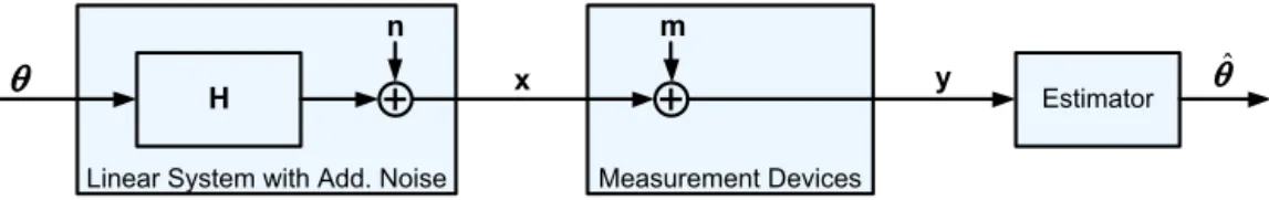
Cost minimization of measurement devices under estimation accuracy constraints in the presence of Gaussian noise

Based on the results obtained in this investigation, it can be concluded that the proposed frictional contact mortar formulation using NURBS-based isogeometric analysis displays

iklim dolabında kurutulan örneklerde kurutma sü- releri, organoleptik nitelikler ve kurutma süresi ile organoleptik niteliklerin etkileşimi sonucu elde edilen puanlar

In this context, we systematically studied blood compatibility of mesoporous silica nanoparticles possessing ionic, hydrophobic or polar surface functional groups, in terms of

Table 4 (page 556) indicates that women with wage work experience outside the household prior to emigration had a greater tendency to become pioneer migrants whereas all

For the edge insertion case, given vertex v, we prune the neighborhood vertices by checking whether they are visited previously and whether the K value of the neighbor vertex is

R,,, L and C, by a Wien-bridge oscillator type circuit and show that this circuit may exhibit chaotic behaviour similar to that of the Chua oscillator.. 2

The most influential factor turn out to be the expectations, which works through two separate channels; the demand for money decreases as the expected level of

Comparison of the examples of works of art given in the Early Conceptual Information Arts section with those dis- cussed in the From Ideas to Knowledge Production (Re- search)