Exciton condensate driven force in double layer systems

EXCITON CONDENSATE DRIVEN FORCE

IN DOUBLE LAYER SYSTEMS

a dissertation submitted to

the graduate school of engineering and science

of bilkent university

in partial fulfillment of the requirements for

the degree of

doctor of philosophy

in

physics

By

Ege ¨

Ozg¨

un

February, 2016

EXCITON CONDENSATE DRIVEN FORCE IN DOUBLE LAYER SYSTEMS

By Ege ¨Ozg¨un February, 2016

We certify that we have read this dissertation and that in our opinion it is fully adequate, in scope and in quality, as a dissertation for the degree of Doctor of Philosophy. Tu˘grul Hakio˘glu(Advisor) Ceyhun Bulutay Afif Sıddıki Balazs Het´enyi Levent Suba¸sı

Approved for the Graduate School of Engineering and Science:

Levent Onural

ABSTRACT

EXCITON CONDENSATE DRIVEN FORCE IN

DOUBLE LAYER SYSTEMS

Ege ¨Ozg¨un Ph.D. in Physics Advisor: Tu˘grul Hakio˘glu

February, 2016

Excitonic systems are challenging to deal with both theoretically and experimen-tally but in return, they offer a very rich physics and exotic features. We will investigate their properties under weak magnetic field and the resultant instabili-ties reminiscent of Sarma-I and Sarma-II phases. A new type of force in condensed matter physics, emerging due to the presence of the excitonic condensation will be demonstrated via semi-analytical and numerical calculations in two different systems of GaAs double quantum well geometries and layered transition metal dichalcogenide material 1T -T iSe2. Competition of charge-density wave and

ex-citon condensate orders in layered systems will also be discussed in detail and an alternative explanation for the periodic lattice distortions observed in 1T -T iSe2

will be posed.

¨

OZET

C

¸ ˙IFT KATMANLI S˙ISTEMLERDE EGZ˙ITON

YO ˘

GUS

¸MASINDAN DO ˘

GAN KUVVET

Ege ¨Ozg¨un Fizik, Doktora

Tez Danı¸smanı: Tu˘grul Hakio˘glu S¸ubat, 2016

Egzitonik sistemler, hem deneysel hem de teorik olarak zorlayıcı sistemlerdir ama bunun kar¸sılı˘gında olduk¸ca zengin bir fizik ve egzotik ¨ozellikler sunarlar. Bu sis-temlerin zayıf manyetik alan altındaki ¨ozelliklerini ve ortaya ¸cıkan, Sarma-I ve Sarma-I benzeri kararsızlıkları inceleyece˘giz. Egziton yo˘gu¸smasının varlı˘gında or-taya ¸cıkan, yo˘gun madde fizi˘gindeki yeni bir tip kuvveti, n¨umerik ve yarı analitik metotlar ile, biri GaAs ¸cift kuvantum kuyusu geometrisi, di˘geri ise katmanlı ge¸ci¸s metali dikalkojenlerinden 1T -T iSe2 olan iki farklı sistemde g¨osterece˘giz. Y¨uk

yo˘gunlu˘gu dalgaları ve egziton yo˘gu¸sması d¨uzenlerinin m¨ucadelesini ve 1T -T iSe2

malzemesinde g¨ozlemlenmi¸s olan periodik sapmalar i¸cin alternatif bir senaryoyu da detaylı bir bi¸cimde inceleyece˘giz.

Anahtar s¨ozc¨ukler : Egziton yo˘gu¸sması, y¨uk yo˘gunlu˘gu dalgaları, ¸cift kuvantum kuyuları.

Acknowledgement

I would like to thank my supervisor Prof. Tu˘grul Hakio˘glu for his supports and for his excellent supervising which has significantly increased my understanding of physics and science. I thank my family for their never-ending support. And finally and most importantly, I would like to thank my love, meaning of my life, Pelin T¨oren for motivating me in completing my thesis and making my life wonderful.

Contents

1 Introduction 1

2 Excitons in a nutshell 4

2.1 Basics of exciton physics . . . 4

2.1.1 Definition of an exciton . . . 4

2.1.2 Electron and Hole Bands . . . 7

2.1.3 Dark-bright excitons and radiative couplings . . . 8

2.1.4 Fundamental symmetries in excitonic systems . . . 9

2.2 Bose-Einstein Condensation of excitons . . . 10

2.2.1 GaAs DQW geometry . . . 10

2.2.2 Second quantization of some related operators . . . 12

2.2.3 Hartree-Fock mean field approximation . . . 13

2.2.4 Derivation of the EC Hamiltonian . . . 14

3 Exciton Condensates Under Weak B-field 16 3.1 Introduction . . . 16

3.2 Robust Ground State and the DX-pockets . . . 17

3.2.1 Microscopic theory . . . 17

3.2.2 Numerical results . . . 22

4 The EC force 27 4.1 Introduction . . . 27

4.2 Condensation free energy and the emergence of the EC force . . . 28

4.3 Numerical Results . . . 29

4.4 Semi-analytical derivation of the EC force . . . 29

CONTENTS _vii

5 EC-CDW Instability Competition and EC-Force in TMDC 36

5.1 Introduction . . . 36

5.2 Theory of CDW Instability . . . 37

5.2.1 CDW Instability in 1D Systems . . . 37

5.2.2 Microscopic Theory of CDW for 2D Systems . . . 41

5.3 A model for CDW and EC orders in layered systems . . . 42

5.4 Results . . . 46

5.4.1 Competition of EC and CDW instability . . . 46

5.4.2 EC-Force in TMDC . . . 47

5.4.3 An Alternative Approach for the Periodic Lattice Distor-tions in 1T -T iSe2 . . . 51

5.4.4 Tuning the transition temperatures via electron-phonon in-teraction . . . 51

6 Conclusion 53

List of Figures

2.1 Simple illustration of Wannier-Mott and Frenkel excitons. a) Wannier-Mott excitons extend to several lattice sites with a weaker attraction between the bound electron-hole pairs. b) Frenkel exci-tons are tightly bound and are limited to a single lattice site. . . . 5 2.2 Conduction electron and valence heavy hole and light hole bands

of GaAs for a band gap of EG = 1.42eV . Horizontal axis is

dimen-sionless wavevector scaled with a2

B and vertical axis is energy in

units of Hartree energy EH = 12meV . . . 7

2.3 Coupled quantum wells of GaAs with the dielectric material AlGaAs for realizing EC state. An electric field E ≃ 50kV /cm is applied in the growth (z) direction to enhance the lifetime of the excitons. . . 11 3.1 E_1k(−)/EH (a) and E2k(+)/EH (b) versus kaB is plotted for n(+)a2B =

0.1, 0.3, 0.5, 0.7 (from bottom to top) at constant n(−) _{= 0 and}

g∗_B/B

0 = 0. . . 23

3.2 E_1k(−)/EH (a) and E2k(+)/EH (b) versus kaB is plotted for g∗B/B0 =

0, 2, 4, 6 (from top to bottom) at constant n(+)_{= 0.1 and n}(−)_{= 0. 24}

3.3 E_1k(−)/EH (a) and E2k(+)/EH (b) versus kaB is plotted for g∗B/B0 =

0, 0.2, 0.4, 1 (from top to bottom) at constant n(+)_{= 1.5 and n}(−) ₌

1.1. . . 25 3.4 E_1k(−)/EH (a) and E2k(+)/EH (b) versus kaB is plotted for n(−) =

0, 0.1, 0.3, 0.5 (from top to bottom) at constant n(+) _{= 0.55 and}

g∗_B/B

LIST OF FIGURES _ix

3.5 E_1k(−)/EH (a) and E2k(+)/EH (b) versus kaB is plotted for n(−) =

0, 0.4, 0.8, 1.4 (from top to bottom) at constant n(+) _{= 1.5 and}

g∗B/B0 = 0.2. . . 26

4.1 The EC OP scaled with Hartree energy versus layer separation D and wavevector k, in units of aB is plotted for n(+)a2B = 0.1. When

critical separation is reached, EC OP diminishes to zero rapidly. . 30 4.2 The EC OP at k = 0 scaled with EH as a function of the

dimen-sionless layer separation D/aB is plotted using the numerical and

semi-analytical calculations. The results show the success of the parabolic approximation in generating the square root behavior of ∆(0) with increasing layer separation. . . 34 4.3 Change of the free energy scaled with the EH as a function of the

dimensionless layer separation D/aBis plotted using the numerical

and semi-analytical calculations. Again the power of the parabolic approximation can be seen from the comparison of numerical and semi-analytical results. . . 35 5.1 The static response functions versus the dimensionless wave vectors

plotted for 1D, 2D and 3D. . . 39 5.2 EC OP, scaled with t0 = 0.125eV , is plotted for different second

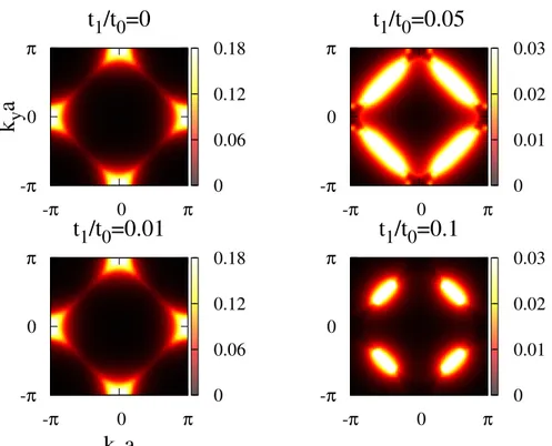
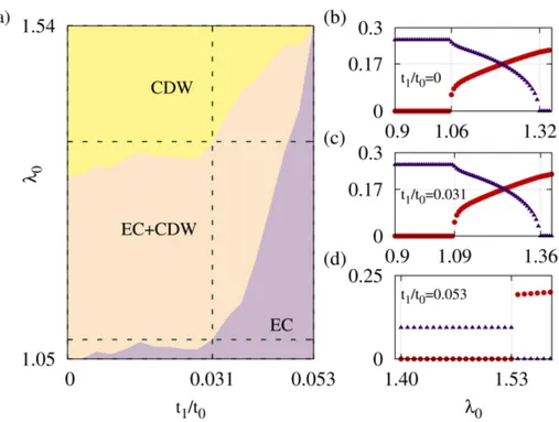
NN interaction strengths. The peak positions of the EC OP are separated by the nesting vector, Q = (±π, ±π) in each of the four cases. For zero or a small second NN interaction, OP is maximum at the saddle points of the dispersion, due to nearly perfect nest-ing. As the second NN interaction increases, the perfect nesting gradually disappears. . . 47 5.3 Color map of the CDW and EC for t1 = 0. The OPs are mapped

via fcol = tan−1[∆max_G ] transformation. In yellow (light) regions

there is only EC and in black (dark) regions only CDW is present, whereas in between they coexist. Here, λ0 runs from 0.9 to 1.6 and

LIST OF FIGURES _x

5.4 Regimes with different coexistence/competition properties are pre-sented for EC and the CDW OPs for varying λ0 and t1. Here,

increasing t1 plays the major role in breaking the optimal nesting

condition which weakens both OPs, whereas t1 and λ0 together

determine two regimes of coexistence/competition as indicated in (a). Several cross sections of (a) are given for the EC and CDW order parameters as, b) t1 = 0: EC OP (blue triangles) gradually

drops to zero with the onset of CDW (red circles), c) t1 = 0.031:

the region of coexistence is narrowed and shifted to higher λ val-ues, and d) t1 = 0.053: a direct transition from EC to CDW, with

no coexistence. The OPs on the vertical scale of (b-d) are given in units of t0. . . 49

5.5 The change in the free energy per area with respect to D/a is plot-ted for different λ0 and t1/t0 values. Free energy becomes constant

after EC vanishes, with only CDW remaining, which means that the EC force is zero beyond that critical point. . . 50 5.6 Transition temperatures of EC (TEC

c ) and CDW (TcCDW) orders

are illustrated for four different λ0 values for n0 ≃ 1014cm−2 and

t1 = 0. a)EC OP has a higher Tc than CDW OP. b) By increasing

λ0 the two critical temperatures were made to coincide at T = Tc∗.

c) After increasing λ0 further, CDW order gains a higher Tc. d)

Increasing λ0 even further, the two Tc’s can be widely separated.

Chapter 1

Introduction

Excitons are composite bosons created by the electron-hole bound state in the semiconductor background. In 1924 S.N. Bose and A. Einstein represented a new phase of matter, the well-known Bose-Einstein condensation[1, 2], in which un-der a critical temperature bosons start to condense in the ground state. It was first Moskalenko, Blatt, Ber and W. Brandt to theoretically suggest in 1960s the Bose-Einstein condensation of a dilute exciton gas[3, 4] also referred as exciton condensation. We will deal with the many body low temperature collective effects in excitonic systems. In particular, dilute exciton gas should Bose-Einstein con-dense at a much higher critical temperature than atomic boson gases, thanks to higher spin degeneracy and lower effective mass. These properties of the exciton gas under sufficiently low temperatures makes the problem still a hot research topic today. The experiments on the condensed state was inconclusive until re-cently. The modern exciton experiments are performed using coupled quantum wells [5, 6, 7, 8] which supplies a factor of 1000-10000 enhancement in exciton life-time compared to the former experiments that were taking place in bulk systems. Despite the advantage in the use of coupled quantum wells, the early experiments have not been totally indicative of a condensed state, leaving room for other ex-planations. The basic reason for this lack of evidence is that, all experiments are based on photoluminescence techniques, therefore only those exciton states that couple to light (the so called bright excitons) can be probed. Recently it is

demonstrated that dark excitons dominate the condensed ground state[9] which cannot be probed by light.

Acknowledging the categorization suggested by Snoke[10], we can present the earlier exciton condensation research under 4 main titles: a) 2D excitons in cou-pled quantum wells b) Coulomb drag experiments in coucou-pled two-dimensional electron gases c) Three-dimensional excitons in the bulk semiconductor Cu2O

d) Polaritons in semiconductor microcavities. In addition to this categoriza-tion, excitons created in different semiconductor quantum wells can be formed by electron-hole pairs within the same band (both conduction or both valence) or in different bands. In the former case, the excitonic subsystem respects the particle-hole symmetry, whereas in the latter this symmetry is absent (due to different band masses as well as orbital and spin properties). Fundamental symmetry con-siderations in the absence of the particle-hole symmetry and their consequences have been studied recently [11, 12]. Experiments in the former case are more common (such as those by Snoke in Ref.[10].) On the other hand, the experi-ments carried out mostly by the Eisenstein group in Caltech[13, 14, 15, 16, 17] that respected the particle-hole symmetry, was enabled by the use of a strong magnetic field, forcing the electrons and holes to share the same type of Lan-dau bands in different wells. Many of the experimental results performed by the Eisenstein and his colleagues have not yet been completely understood , among which are the Hall drag quantization, the presence of a sharp critical layer sep-aration, zero bias tunneling, topological phases, superfluidity etc. In addition to these unsolved problems, it has been recently suggested that a new type of force may be present at the phase boundary (the boundary separating the condensed state from the normal exciton gas) reducing its strength (but never to zero) deep inside the condensed state[9, 18].

The longly sought evidence for the condensed state came recently by the obser-vation of the interference fringes arising from the excitonic condensate’s macro-scopic wavefunction[19].

Our main interest is to device alternative and satisfactory theoretical methods for conclusive observation of the excitonic condensed state in coupled quantum

wells. In particular, we will be investigating the effect of the weak magnetic fields on the condensed state, predicting the magnitude of this new force both numerically and semi-analytically.

In Chapter 2, we will lay the basics of the excitonic systems and device the tools to handle them. Chapter 3 is devoted to the effects of a weak magnetic field on the excitonic condensate. In Chapter 4, we will start investigating the new force aris-ing in the excitonic systems i.e. exciton condensate force (EC-force). Chapter 5 deals with the exciton condensate force and charge-density wave instability/exci-ton condensation competition in layered transition metal dichalcogenide material 1T -T iSe2. We will conclude with Chapter 6.

Chapter 2

Excitons in a nutshell

2.1

Basics of exciton physics

2.1.1

Definition of an exciton

An exciton is similar to a hydrogen atom, in which the proton is replaced by a hole i.e., excitons are bound states of electron-hole pairs. There are two different types of excitons; Frenkel excitons[20] and Wannier-Mott excitons[21, 22]. The difference between these two types of excitons is in the attraction holding them together. Since the magnitude of the attraction determines the separation be-tween the electrons and holes, these two types will also acquire different exciton Bohr radius aB values. Exciton Bohr radius is defined in a similar manner to the

Bohr radius for the Hydrogen atom. We can follow the standard procedure to derive an expression for aB. First we equate the Coulomb force to the rotational

force: e2 4πǫr2 = m ∗ eω2r (2.1) where e, ǫ, r, m∗

Figure 2.1: Simple illustration of Wannier-Mott and Frenkel excitons. a) Wannier-Mott excitons extend to several lattice sites with a weaker attraction between the bound electron-hole pairs. b) Frenkel excitons are tightly bound and are limited to a single lattice site.

the electron and the hole, effective electron mass and angular frequency of the electron respectively. We can recast this equation by substituting ω = v/r where v is the velocity and multiplying both sides by mr and using the Bohr-Sommerfeld quantization condition L = n¯h, we have:

r = 4πǫ¯h

2

m∗ ee2

n2 (2.2)

Finally, setting n = 1 for the state with the lowest energy, i.e., ground state, we obtain the expression for the exciton Bohr radius:

aB =

4πǫ¯h2 m∗

ee2

(2.3) Let us now return to the discussion of Frenkel and Wannier-Mott excitons. Frenkel excitons are tightly bound electron-hole pairs with exciton Bohr radii

of the order of a single lattice spacing, whereas Wannier-Mott excitons are their loosely bound counterparts with exciton Bohr radius values acquiring several lat-tice spacings. Different types of materials give rise to different types of aB values,

since different materials have different dielectric constants and different effective band masses. We will investigate these different cases in detail in the following chapters.

It is important to define the notion of composite bosons while tackling with the excitonic systems. Electrons and holes are both fermions; by the simple angular momentum addition rules it is known that two fermions adds upto a boson. In the language of group theory, it is cast as follows:

1 2 ⊗

1

2 = 0 ⊕ 1 (2.4)

The detailed explanation of angular momentum summation rules within the con-text of group theory can be found in Ref. [23] for instance. So excitons, which are bound states of electron-hole pairs, can be treated as composite bosons under certain conditions. We basically need to consider two quantities to determine whether our excitons can be treated as composite bosons or not: a) the exciton density n(+) _{b) the exciton Bohr radius a}

B. The limiting condition comes from

the commutation relation of the exciton operators[24]:

[ck,σ, c†k′_,σ′] = δk,k′δ_σ,σ′ + O(n(+)a3_B) (2.5)

where ck,σ/c†k,σ are bosonic exciton annihilation/creation operators built from

the multiplication of two fermionic operators, k is the wavevector, σ is the spin index, and δ denotes the Kronecker delta. The above equation is a valid bosonic commutation relation if n(+)a3B ≪ 1. This relation is generalized to d-dimensions

by using the d-dimensional exciton density and ad

B. Throughout this thesis, we

will focus on the two-dimensional case. Recasting the above condition in 2D we have:

n(+)a2_B ≪ 1 (2.6)

We will consider two different cases of n(+) _{∼ 10}14 _cm−2_{, a}

B = 5˚A and n(+) ∼

1011_{− 10}12 _cm−2_{, a}

2.1.2

Electron and Hole Bands

Electrons and holes acquire effective band masses, when they are in semiconduc-tors. There exist three main bands: electron band (conduction), light hole band (valence) and heavy hole band (valence). We will mostly deal with GaAs double quantum well (DQW) semiconductors. In these III-V semiconductors of GaAs, the typical effective masses for the aformentioned bands are given as:

m∗_e = 0.067m0 m∗hh= 0.45m0 m∗lh = 0.082m0 (2.7)

with m0 being the electron mass in vacuum and subindices e, hh, lh denoting

electron, heavy hole, light hole respectively. A simple illustration of these bands in GaAs with a band gap of EG = 1.42eV (at 300K) is given in Fig2.2.

e-band

hh-band

lh-band

Figure 2.2: Conduction electron and valence heavy hole and light hole bands of GaAs for a band gap of EG = 1.42eV . Horizontal axis is dimensionless wavevector

scaled with a2

B and vertical axis is energy in units of Hartree energy EH = 12meV

2.1.3

Dark-bright excitons and radiative couplings

Electrons and holes, being fermions, have their spin, S = 1/2. Electrons coming from s-like conduction bands carry angular momentum L = 0 and heavy holes coming from p-like bands carry angular momentum L = 1. This results in elec-trons with total angular momenta J = 1/2 and holes with total angular momenta J = 3/2. To be more specific, heavy holes have Jz = ±3/2 and light holes have

Jz = ±1/2. The lowest energy combinations give the following combinations for

the excitons:

| ↑↑i = |2 2i | ↓↓i = |2 − 2i | ↑↓i = |1 − 1i | ↓↑i = |1 1i

These combinations give rise to two fundamentally different varieties, i.e. dark and bright excitons. Bright excitons couple to the light with their odd total angular momenta whereas their dark counterparts are invisible to light with their even angular momenta. Different coupling properties of the dark and bright excitons lead to an important result in the condensed phase: Due to the finite life time of excitons, electron-hole pairs recombine and emit radiation in the form of a photon. The emitted photon can interact with the dark and bright exciton branches via the radiative dipole couplings and as the result of this coupling the amount of bright states in the ground state (GS) diminishes drastically, leaving a purely dark GS[9]. Although there are higher order corrections coming from the Shiva diagrams[25, 26] i.e., dark-bright exchange interactions, in detailed balance the GS is dominated by the dark excitons. This resulted in a huge problem for the experiments based on photoluminescence measurements, since dark states do not couple to the light, which delayed the longly sought experimental evidence of the condensed phase until the pioneering work of Butov et al.[19]

2.1.4

Fundamental symmetries in excitonic systems

There are two fundamental symmetries for the excitonic systems to consider: fermion exchange symmetry (FX) and time reversal symmetry (TRS)[11, 12]. Let us begin with FX which is analogous to the particle-hole symmetry (PHS). In the excitonic systems if FX is respect then the below relations must hold:

∆↑↑(k) = Che†k↑h † −k↑i = Chh † −k↑e † k↑i = −∆↑↑(−k) ∆↑↓(k) = Che†k↑h † −k↓i = Chh † −k↓e † k↑i = −∆↓↑(−k) ∆↓↑(k) = Che†k↓h † −k↑i = Chh † −k↑e † k↓i = −∆↑↓(−k) ∆↓↓(k) = Che†k↓h † −k↓i = Chh † −k↓e † k↓i = −∆↓↓(−k)

where ∆σσ′ denotes the order parameter (OP) for the exciton condensate, C

includes all of terms relating thermodynamic average of fermionic operators to the OP that are absent in the above equation and ↑ / ↓ denotes spin quantum numbers. So when we have FX, using the above equation we can write:

¯

∆(k) = − ¯∆T(−k), ∆¯(k) = ∆↑↑(k) ∆↑↓(k) ∆↓↑(k) ∆↓↓(k)

!

(2.8) At this point, the interaction will determine whether we will have singlet or triplet states in our system. If we have an even interaction for instance, we have:

¯

∆(k) = ¯∆(−k) (2.9)

In that case, ∆↑↑(k) = ∆↓↓(k) = 0 and ∆↑↓(k) = −∆↓↑(k) so we have real singlet

terms surviving, with all triplet terms vanishing. This is exactly what we have in the case of conventional superconductivity (CSC). If FX were absent in CSC, then one would need to include the triplet terms in addition to the real singlet OP. In the opposite case, an odd interaction yields:

¯

∆(k) = − ¯∆(−k) (2.10)

which gives ∆↑↓(k) = ∆↓↑(k) leaving dz 6= 0, ∆↑↑(k) and ∆↓↓(k). Let us now

move to the other important symmetry within the context of EC, which is TRS. Time reversal operator ˆΘ is an antiunitary operator and has three effects on a complex function: it complex conjugates it, it inverts the wavevector k and it

inverts the spin σ. Because of its antiunitary nature, ˆθ2 _{= −1 which gives rise to}

the following: ˆθ :↑= − ↓ and ˆθ :↓=↑. The choice of the minus sign in the former equation here is arbitrary and can also be put in the latter equation instead. Considering these carefully, we have:

ˆ Θ : ∆↑↑(k) ∆↑↓(k) ∆↓↑(k) ∆↓↓(k) ! = ∆ ∗ ↓↓(−k) −∆∗↓↑(−k) −∆∗ ↑↓(−k) ∆↑↑(−k) ! (2.11) Again the interaction determines the destiny of the singlet and triplet OPs. In the case of a real even interaction we have, ∆↑↑(k) = ∆↓↓(k) and ∆↑↓(k) = −∆↓↑(k),

a real odd interaction yields ∆↑↑(k) = ∆↓↓(−k) and ∆↑↓(k) = ∆↓↑(k). Finally

lets investigate FX and TRS together.

When both FX and TRS manifest and we have a real even interaction we end up with a real singlet: ∆↑↑(k) = ∆↓↓(k) = 0 and ∆↑↓(k) = −∆↓↑(k). For the

case of real odd interaction ∆↑↑(k) = −∆↓↓(k) and ∆↑↓(k) = ∆↓↑(k)

Lets conclude this section by briefly talking about the cases when these sym-metries are manifest or broken. The FX is broken in the DQW excitonic systems since there are two species of fermions in excitonic systems. The FX can be manifest in double layer systems with half filled wells, but in that case it is more convenient to talk about PHS instead of FX. The TRS is manifest in the absence of magnetic field but it can also be spontaneously broken.

2.2

Bose-Einstein Condensation of excitons

2.2.1

GaAs DQW geometry

We will use two different geometries; GaAs DQW geometry and 1T -T iSe2, a

layered transition metal dichalcogenide. Let us reserve the latter one for later and briefly discuss the former one for now. The GaAs DQW geometry consists of two

Figure 2.3: Coupled quantum wells of GaAs with the dielectric material AlGaAs for realizing EC state. An electric field E ≃ 50kV /cm is applied in the growth (z) direction to enhance the lifetime of the excitons.

GaAs quantum wells and a dielectric material, AlGaAs in between, separating the wells. Typical values for the separation is ∼ 100˚A. First a laser is shone to create the electron hole pairs. Since electrons and holes tend to recombine, the lifetime of excitons is extremely short, on the order of nano meters. An electric field with magnitude ≃ 50kV /cm is applied in the growth direction (z-direction), to enhance coupling of the electron hole pairs by tuning the valence p and conduction s bands. By this procedure, nearly a thousand fold enhancement in the lifetime is achieved. Then the system is cooled to the temperatures below the EC transition temperature TEC

2.2.2

Second quantization of some related operators

While dealing with many particle quantum systems, it is advantageous to use the second quantization formalism. Lets start with the kinetic energy operator. In real space, the second quantized kinetic energy is given as (for the discussion of first and second quantization and transition between them there are plenty of references, see for instance Ref.[27]):

ˆ H0 = X σ Z dr ψσ(r)εrψσ†(r) (2.12)

in which εr = −¯h2/2m∇2r, ψσ(r) and ψσ†(r) are the real-space

annihilation/cre-ation operators at position r with spin σ. Now lets write the real space annihila-tion/creation operators in reciprocal space, using the Bloch basis:

ψσ(r) = X k ek,σeik·r (2.13) ψ_σ†(r) = X k e†_k,σe−ik·r (2.14)

in the above equations ek,σ/e†k,σ are the annihilation/creation operators with

mo-mentum k and spin σ. Plugging those Fourier transformations into Eq.(2.12), we have: ˆ H0 = X k,k′_,σ eik·r− ¯h 2 2m∇ 2 re −ik′_·r ek,σe†k′_,σ = X k,k′_,σ εk δk,k′e_k,σe†_k′_,σ ˆ H0 = X k,σ εk ek,σe†k,σ (2.15)

where εk is the energy-momentum dispersion. This is the most general form of

the second quantized kinetic energy operator. Now lets move on to the derivation of the most general two-body interaction term in second quantized language with the only condition that v(r − r′_{) depends only on |r − r}′_|:

ˆ H1 = 1 2 X σ,σ′ Z dr Z dr′ ψσ(r)ψ†σ(r)v(r − r′)ψσ′(r′)ψ†_σ′(r ′_{) (2.16)}

Factor of 1/2 is introduced to avoid double counting. Again expanding the real space operators in the Bloch basis:

ˆ H1 = 1 2 X σ,σ′ X k1,k2,k3,k4 Z dr Z dr′ ei(k1−k2)·r v(r − r′) ×

ei(k3−k4)·r′ ek1,σe † k2,σek3,σ′e † k4,σ′ (2.17)

At this point we will use a Jacobian preserving transformation by defining r− =

r−r′ _{and r}

+ = (r+r′)/2. Recasting the above equation using this transformation

yields: ˆ H1 = 1 2 X σ,σ′ X k1,k2,k3,k4 Z dr₊ Z dr₋ e2i(k1−k2−k3+k4)·r−_v(r +) × (2.18) ei(k1−k2+k3−k4)·r+_e k1,σe † k2,σek3,σ′e † k4,σ′

Fourier transforming the interaction term and using the spectral definition of the delta function we have:

ˆ H1 = 1 2A X σ,σ′ X k,k1,k2,k3,k4 v(k)δ2k+k1−k2−k3+k4δk1−k2+k3−k4ek1,σe † k2,σek3,σ′e † k4,σ(2.19)′

where A is the area and comes from the Fourier transform of v(r+) (since we

will be dealing with effectively 2D systems, the derivations are made for that case). Performing the k4 and k2 sums by respecting the momentum conservation

conditions, k4 = −2k−k1+k2+k3and k2 = k+k1we obtain the final expression

for the second quantized two body interaction: ˆ H1 = 1 2A X σ,σ′ X k,k′_,q v(q)e†_k+q,σe†k′_−q,σ′ek′_,σ′e_k,σ (2.20)

in which, dummy indices are redefined and anticommutation relations of fermionic operators are used. Factors of 2π’s coming from the Fourier transformations are omitted during these derivations, since they cancel out with the 2π’s coming from Kronecker deltas.

2.2.3

Hartree-Fock mean field approximation

We will use the general two-body interaction in Eq. (2.20) to describe the excitonic systems. One difficulty arises when we want to calculate the eigenspectrum of our system. The problem appears due to the four fermionic operators in ˆH1. Using

neglect the fluctuations of order two, we can recast the second quantized two-body interaction term in a form that allows us to solve it self-consistently. To do so, lets first rewrite the most general case of four fermionic operators:

e†keke†k′ek′ = e†_ke_khe†_k′ek′i + he†_ke_kie†_k′ek′ − he†_ke_kihe†_k′ek′i + σ_kσ_k′ (2.21)

where σk = e†kek− hek†eki is the fluctuations of e†kek around its mean. The last

term in the above equation is second order in fluctuations so we neglect that term. The third term does not affect the diagonalization of the Hamiltonian, it only contributes to the total energy. We will see that in the case of exciton conden-sation (EC), this term is going to be the condenconden-sation (free) energy. So we can also drop this term out while calculating the eigenspectrum of our Hamiltonian. The remaining two terms, together with the equations for he†keki and he†k′ek′i,

can be solved self-consistently. The equations for these thermodynamic averages corresponds to the (OP) equations for the ordered systems, which in our case is the equation for the EC OP.

2.2.4

Derivation of the EC Hamiltonian

Now we are in a position to present a microscopic theory for the EC. Our Hamilto-nian consists of kinetic energy terms for the electrons and holes and the Coulomb interaction term: ˆ H = Hˆ(e)+ ˆH(h)+ ˆH(eh) ˆ H(e) = X kσ ξk(e)e † k,σek,σ ˆ H(h) = X kσ ξ_k(h)h†_−k,σh−k,σ ˆ H(eh) = 1 A X σ,σ′ X k,k′_,q veh(q)e†k+q,σh † k′_−q,σ′ek′_,σ′h_k,σ with, ξ_k(e) = ¯h 2_k2 2m∗ e − µe+ Σ(e)k ξk(h) = ¯h2k2 2m∗ h − µh+ Σ(h)k

where veh(q) = −e2e−|k−k ′_|D

/(2ǫ|k − k′_{|) is the Fourier transform of the Coulomb}

potential v(r − r′_{) = e}2_{/(4πǫ|r − r}′_{− De}

z|), with D being the layer separation

between the electron and hole wells, µeand µh are the electron and hole chemical

potentials, Σ(e)_k and Σ(h)_k are the electron and hole self energies which we will derive next together with the Coulomb term using Hartree-Fock mean field theory. For the EC order, the pairings with lowest energies are of those with zero center of mass momentum, i.e. we have k′ _{= −k. Eliminating the k}′ _{sum and rearranging}

the indices we have the following for the interaction term: ˆ H(eh) = 1 A X σ,σ′ X k,k′ veh(k − k′)e†k′_,σh † −k′_,σ′ek,σ′h_k,σ (2.22)

The self energy terms arise from the elecron-electron type of interactions with the condition k′ _{= k + q and is given by:}

ˆ H(ee)= 1 2A X σ,σ′ X k,k′ vee(k − k′)e†k′_,σh † k′_,σ′ek,σ′h_k,σ (2.23)

Here the electron-electron interaction given by vee(k − k′) = −e2/(2ǫ|k − k′|) is

Using the mean field approach on the above equations we obtain the final form of our Hamiltonian: ˆ H = X kσσ′ h ξk(e)e † k,σek,σ+ ξk(h)h † −k,σh−k,σ+ ∆σσ′(k)e_k,σh_k,σ+ h.c i (2.24) ∆σσ′(k) = 1 A X k′ veh(k − k′)he†k′_,σh † −k′_,σ′i (2.25) Σ(e)k = 1 2A X k′ vee(k − k′)he†k′_,σek′_,σi (2.26) Σ(h)_k = 1 2A X k′ vee(k − k′)hh†k′_,σhk′_,σi (2.27)

where ∆σσ′(k) are the EC OPs and the constant term he†_k′_,σh †

−k′_,σ′ihek,σ′h_k,σi

coming from the mean field approximation is omitted. We will concentrate on this term while calculating the EC force.

Chapter 3

Exciton Condensates Under

Weak B-field

3.1

Introduction

Excitonic systems present quite a wide spectrum of interesting features thanks to the absence/presence of FX symmetry, unconventional coupling between two species of fermions, k-dependent OP and manipulation of the GS by the exter-nal fields. For instance, when a magnetic field is turned on, TRS is broken and the Kramers degeneracy in the eigenspectrum is lifted. A more interesting phe-nomenon in that case is the robustness of the condensed GS against the weak fields: The GS remains unchanged until a critical field strength is reached. When this critical field strength Bc is reached, another significant result is obtained

where instabilities arise yielding negative energy states, i.e de-excitation pockets (DX-pockets)[30]. These states are analogous to the negative energy states re-ported by Sarma in the early 60’s[31]. Analytical studies of these instabilities, i.e. Sarma-I and Sarma-II phases and also LOFF phases were reported for the atomic condensates[32, 33, 34, 35, 36]. LOFF phases are not included in this thesis, which are instabilities arising from non-zero center of mass momentum pairings, which

can be triggered by a strong magnetic field in superconductor systems for in-stance and requires real space diagonalization, which was not achieved for the EC systems yet to our knowledge.

3.2

Robust Ground State and the DX-pockets

3.2.1

Microscopic theory

Lets recast Eq.(2.24) in the matrix form using the (e†_k↑e†_k↓h−k↑h−k↓) basis:

ˆ H =X k        ξ_k(e) 0 ∆∗ ↑↑(k) ∆∗↓↑(k) 0 ξk(e) ∆∗↑↓(k) ∆∗↓↓(k) ∆↑↑(k) ∆↑↓(k) ξk(h) 0 ∆↓↑(k) ∆↓↓(k) 0 ξk(h)        (3.1)

By defining ε(+)_k = (ξ_k(e)+ ξ_k(h))/2 and ε(−)_k = (ξ_k(e)− ξ_k(h))/2 we can rewrite the above equation in the following form:

ˆ H =X k ( ε(−)k σ0 ⊗ σ0 + ε(+)k σ0 ∆¯†(k) ¯ ∆(k) −ε(−)k σ0 ! ) (3.2) in which σ0 is the 2×2 unit matrix, ¯∆(k) is the OP matrix[28], which was also

in-troduced in the previous chapter. The energy spectrum of the above Hamiltonian is two-fold degenerate and given by:

λ(±)_k = ε(−)_k ± λk = ε (−)

k ±

q

[ε(+)_k ]2_{+ tr[ ¯∆(k) ¯∆}†_{(k)]/2 (3.3)}

To find the eigenfunctions, we need to diagonalize this Hamiltonian. For that, we will resort to an unitary transformation:

ˆ

U ˆH ˆU† _{= ˆH}

d (3.4)

where ˆHd is the diagonalized Hamiltonian, and ˆU is the unitary transformation

we are using and are given by: ˆ Hd= λkσ0 0 0 −λkσ0 ! , U =ˆ        αk 0 βk γk 0 αk −γk βk −βk γk αk 0        (3.5)

Multiplying both sides of Eq.(3.4) by ˆU from the right, we have a set of equations for αk, βkand γk. Combining these with the equations coming from the unitarity

condition ˆU ˆU† _{= σ} 0⊗ σ0 we have: αk = Ck[λk+ ε(+)k ] βk = Ck∆↑↑(k) γk = Ck∆↑↓(k) Ck = 1 q 2λk[λk+ ε(+)k ]

Since we determined the elements of ˆU we can now also find the new basis in which our Hamiltonian is diagonal:

       g1k g2k g_3k† g_4k†        =        αk 0 βk γk 0 αk −γk βk −βk γk αk 0 −γk −βk 0 αk               ek↑ ek↓ h†_−k↑ h†_−k↓        (3.6)

multiplying by ˆU† _{from the left we can also express our old basis in terms of the}

new one:        ek↑ ek↓ h†_−k↑ h†_−k↓        =        αk 0 −βk −γk 0 αk γk −βk βk −γk αk 0 γk βk 0 αk               g1k g2k g_3k† g_4k†        (3.7) or in open form: ek↑ = αkg1k− βkg3k† − γkg4k† ek↓ = αkg2k+ γkg_3k† − βkg†_4k h†_−k↑ = βkg1k− γkg2k− αkg3k† h†_−k↓ = γkg1k+ βkg2k+ αkg†4k

and similarly for the quasiparticle operators we have: g1k = αkek↑+ βkh†_−k↑+ γkh†_−k↓

g2k = αkek↓− γkh†−k↑+ βkh†−k↓

g3k = αkhk↑− βke†−k↑+ γke†−k↓

By using the TRS transformation properties of the OPs, we can relate the quasi-particle annihilation operators: OPs in our case are real and since the Coulomb potential is even we have: ˆΘ : ∆σσ(k) = ∆σ ¯¯σ(k) and ˆΘ : ∆σ¯σ(k) = −∆σσ¯ (k).

Using these in the above equations we obtain the following transformations: ˆ Θ : g1k = g2(−k) ˆ Θ : g3k = g4(−k) ˆ Θ : g2k = −g1(−k) ˆ Θ : g4k = −g3(−k)

We can express the GS similar to the product state defined in the BCS theory[29] via the vacuum modes:

|Ψ0i = Y k |Ψki, |Ψki = Tk(1)T (2) k |0i (3.8) with Tk(1) = αk− βke†_k↑h†_−k↑− γke†_k↑h†_−k↓ T_k(2) = αk− βke†k↓h † −k↓+ γke†k↓h † −k↑

The ground state has two significant features. Firstly, it is a singlet, i.e. |Ψki =

|Ψ−ki and secondly, it transforms to itself under time reversal.

Before advancing to the derivation of the self consistent set of equations, let us write the diagonalized Hamiltonian via the ground state energy EG:

ˆ Hd= EG+ X k [λ(+)k (g † 1kg1k+ g†2kg2k) − λ(−)k (g † 3kg3k+ g†4kg4k)] (3.9)

where the ground state energy is given by: EG = 2

X

k

λ(−)_k (3.10)

From this moment, we will take dark and bright EC OPs to be equal by ignoring the radiative coupling which yields: |∆↑↑(k)| = |∆↓↓(k)| = |∆↑↓(k)| = |∆↓↑(k)|

and denote this single OP simply by ∆(k). Since we know the transformation between the old and the new basis we can easily cast the OP equation using Eq.(2.25): ∆(k) = 1 Z dk′ v(k − k′)∆(k ′₎ [f1(k′) − f2(k′)] (3.11)

where, f1(k) and f2(k) are the Fermi-Dirac functions for energies λ(+)k and λ (−) k

respectively. To complete the self consistent set, we need number conservation equations and self energies. Number conservation for the electrons and holes are given by: N(e) = X kσ he†_kσekσi (3.12) N(h) ₌ X kσ hh†_kσhkσi (3.13)

where N(e) _{and N}(h) _{are number of electrons and holes respectively. Calculating}

those thermodynamic averages we have: n(e) = Z dk (2π)2 h (1 + ε (+) k λ(k))f1(k) + (1 − ε(+)k λ(k))f2(k) i (3.14) n(h) = Z _dk (2π)2 h (1 − ε (+) k λ(k))  1 − f1(k)  + (1 + ε (+) k λ(k))  1 − f2(k) i (3.15) in which n(e) _{= N}(e)_{/A and n}(h) _{= N}(h)_{/A are the electron and hole densities.}

We also need the self energies for the self consistent solution: Σ(e)_k = 1 2 Z dk′ (2π)2vee(k − k ′₎h (1 + ε (+) k λ(k))f1(k) + (1 − ε(+)_k λ(k))f2(k) i (3.16) Σ(h)_k = 1 2 Z dk′ (2π)2vee(k − k ′₎h (1 − ε (+) k λ(k))  1 − f1(k)  + (1 + ε (+) k λ(k))  1 − f2(k) i (3.17) Above equations together with the OP equation form a self consistent set for ∆(k), Σ(e)_k , Σ(h)_k , µe and µh. Alternatively, we can use the exciton density

n(+) _{= (n}(e)_{+ n}(h)_{)/2 and electron-hole density mismatch n}(−) _{= (n}(e)_{− n}(h)_)/2

to solve for ∆(k), Σ(e)_k , Σ(h)_k , µ+ = (µe + µh)/2 and µ− = (µe − µh)/2 self

consistently: n(+) = Z dk (2π)2 h 1 + ε (+) k λ(k)[(f1(k) − f2(k)) i (3.18) n(−) = Z dk (2π)2 h f1(k) + f2(k) − 1 i (3.19) Following the onset of the condensate we turn on a weak magnetic field B(r) = B⊥ˆeφ+Bzeˆz where the radial and perpendicular components of the magnetic field

B⊥and +Bzare independent of θ ans φ and a slowly varying function of r. We are

not considering the effects of the magnetic vector potential which is valid since the magnitude of the magnetic fields we are using are not exceeding and the critical value for the Landau degeneracy, i.e. |B(r) ≪ B0 = φ0nx in which φ0 = h/e

is the flux quantum. We are also neglecting the the influence of light holes on the heavy hole states[37, 38]. The Zeeman coupling for the electron-heavy hole coupled system is given by:

Vz = −(γeσ¯(e)· B(r) + γhσ(h)z Bz) (3.20)

with ¯σ = σxeˆx+σyeˆy+σzˆezdenoting the Pauli matrices, γp = g∗µ∗B, p = (e, h) g∗ =

q

g2

⊥+ gz2 is the effective g-factor and µ∗B = e¯h/2m∗ with m∗ being electron and

hole effective masses for γeand γhrespectively. We will treat the Zeeman coupling

within the first order perturbation theory, and introduce it to the diagonalized EC Hamiltonian in the following manner:

HB = Hd+ Z, Z =

Z(1) ₀

0 Z(2)

!

(3.21) in which Z(i) _{= h}i_{· ¯σ, h}i _{= h}(i)

x eˆx+ h(i)y ˆey+ h(i)z eˆz, i = (1, 2) with h(i)’s given by:

h(1)x = α2kγeB⊥(e)cosφ

h(1)_y = α2_kγeB⊥(e)sinφ (3.22)

h(1)_z = α2kγeBz(e)− (βk2+ γk2)γhBz(h)

given in (g1k, g2k) basis and

h(2)_x = (β_k2+ γ_k2)γeB⊥(e)cosφ

h(2)_y = (βk2+ γk2)γeB⊥(e)sinφ (3.23)

h(2)_z = (β_k2+ γ_k2)γeBz(e)− α2kγhBz(h)

given in (g_3k† , g†_4k) basis. The Zeeman field breaks the degeneracy and splits the energy spectrum into four given by: E_1k(±) = λ(+)_k ± z_k(1) and E_2k(±) = λ(−)_k ± z_k(2) with z_k(1) = |h(1)_{| and z}(2)

k = |h(2)|. The new basis in which HB is diagonal is

related to the EC basis via another unitary transformation:

       G1k G2k G3k        =        cosθ1 2 e −iφ_sinθ1 2 0 0

−eiφsinθ1

2 cos θ1 2 0 0 0 0 cosθ2 2 e−iφsin θ2 2               g1k g2k g3k        (3.24)

with θ1 =

q

(h(1)x )2+ (h(1)y )2/h(1)_z and θ2 =

q

(h(2)x )2+ (h(2)y )2/h(2)_z . Now lets recast

HB in the diagonalized basis:

HB= EG+ X k [E_1k(+)G†_1kG1k+ E1k(−)G † 2kG2k− E2k(+)G † 3kG3k− E2k(−)G † 4kG4k](3.25) in which EG = 2Pkλ (−)

k is the same ground state that we found for the B = 0

case. The ground state is robust against magnetic field unless E_2k(+) becomes positive or E_1k(−) becomes negative at some k values for some critical field Bc.

When it is the case, EG is not the ground state anymore and negative

excita-tions, which we call DX-pockets arise. DX-pockets also arise by introducing a nonzero electron-hole density mismatch. All these cases are investigated in the next section. We can again express the new ground state via a product state:

|ΨBi = Y {k1} G†_2k1 Y {k2} G†_3k2|Ψ0i (3.26)

in the above equation, {k1} and {k2} are the DX-pockets created where E1k(−) < 0

and E_2k(+) > 0 respectively. For these k values it is energetically more favorable to break a pair by the operators G†_2k and G†_3k yielding a new ground state with a negative energy. The DX-pockets corresponding to the E_1k(−)branch have 0 < k < Q1and therefore have disk topology whereas the remaining DX-pockets belonging

to E_2k(+) branch have Q2 < k < Q3 and have ring topology as a result, with Qi’s

designating the positions of the zero energy crossings. These two topologically different instabilities are analogous to the Sarma-I and Sarma-II phases appearing in the BSC systems[31].

3.2.2

Numerical results

We solved the self consistent set of Eqs.[3.11, 3.14, 3.15, 3.16, 3.17] numerically for a parameter space consisting of the dimensionless parameters n(+)_a2

B, n(−)a2B

and g∗_B/B

0. The results are illustrated in Fig. (3.1 - 3.5).

In the absence of electron-hole density mismatch and magnetic field, the ground state is robust and we don’t have DX-pockets as shown in Fig. (3.1). As we turn

on the magnetic field, DX-pockets appear for certain k values, which were denoted by {k1} and {k2} in the previous section and are shown in Fig. 3.2a/Fig. 3.3a

and Fig. 3.2b/Fig. 3.3b, with disk and ring topologies respectively.

The other way to obtain negative energy DX-pockets is to introduce electron-hole density mismatch. When n(−)_a2

B 6= 0, DX-pockets arise for the certain set of

kvalues, which corresponds to the pairs broken by the operators G†_2k1 and G † 3k2.

Those cases are shown in Fig. 3.4 and Fig. 3.5.

0

1

2

3

4

5

6

7

8

9

0 0.5 1 1.5 2 2.5 3

ka

(a)

(b)

a

n

=0, g

B/B

=0

0

0.2

0.4

0.6

0.8

1

1.2

1.4

1.6

0 0.5 1 1.5 2 2.5 3

ka

(a)

(b)

a

n

=0, g

B/B

=0

Figure 3.1: E_1k(−)/EH (a) and E2k(+)/EH (b) versus kaB is plotted for n(+)a2B =

-1

0

1

2

3

4

5

6

7

8

9

0 0.5 1 1.5 2 2.5 3

ka

(a)

(b)

a

n

=0.1, a

n

=0

-0.4

-0.2

0

0.2

0.4

0.6

0.8

1

1.2

1.4

1.6

0 0.5 1 1.5 2 2.5 3

ka

(a)

(b)

a

n

=0.1, a

n

=0

Figure 3.2: E_1k(−)/EH (a) and E2k(+)/EH (b) versus kaB is plotted for g∗B/B0 =

-3

-2

-1

0

1

2

3

4

0 0.5 1 1.5 2 2.5 3

ka

(a)

(b)

a

n

=1.5, a

n

=1.1

-2

-1.5

-1

-0.5

0

0.5

1

1.5

0 0.5 1 1.5 2 2.5 3

ka

(a)

(b)

a

n

=1.5, a

n

=1.1

Figure 3.3: E_1k(−)/EH (a) and E2k(+)/EH (b) versus kaB is plotted for g∗B/B0 =

0, 0.2, 0.4, 1 (from top to bottom) at constant n(+) _{= 1.5 and n}(−) _{= 1.1.}

-1

0

1

2

3

4

5

6

7

8

0 0.5 1 1.5 2 2.5 3

ka

(a)

(b)

a

n

=0.55, g

B/B

=0

0

0.2

0.4

0.6

0.8

1

1.2

1.4

1.6

1.8

2

0 0.5 1 1.5 2 2.5 3

ka

(a)

(b)

a

n

=0.55, g

B/B

=0

Figure 3.4: E_1k(−)/EH (a) and E2k(+)/EH (b) versus kaB is plotted for n(−) =

0, 0.1, 0.3, 0.5 (from top to bottom) at constant n(+)_{= 0.55 and g}∗_B/B 0 = 0.

-1

0

1

2

3

4

5

0 0.5 1 1.5 2 2.5 3

ka

(a)

(b)

a

n

=1.5, g

B/B

=0.2

-0.4

-0.2

0

0.2

0.4

0.6

0.8

1

0 0.5 1 1.5 2 2.5 3

ka

(a)

(b)

a

n

=1.5, g

B/B

=0.2

Figure 3.5: E_1k(−)/EH (a) and E2k(+)/EH (b) versus kaB is plotted for n(−) =

0, 0.4, 0.8, 1.4 (from top to bottom) at constant n(+)_{= 1.5 and g}∗_B/B

Chapter 4

The EC force

4.1

Introduction

The main focus of this thesis which is a recently discovered feature of the EC systems arises due to the D- dependence of the condensation free energy. This feature yields a new type of force i.e. EC force[9, 18] which is reminiscent of the attractive Casimir force (CF) arising between infinitely large metallic plates of identical size[39]. An analogous effect is the Critical Casimir force (CCF), which has been predicted[40] and measured experimentally[41, 42, 43] in binary liquid mixtures. CCF in BEC systems was also speculated[44, 45], but has not yet been observed. However, Casimir-Polder like force between a BEC and a semiconductor plane was measured[46, 47].

As we discussed earlier, there exists two different type of excitons, i.e. dark and bright excitons and due to the radiative corrections, bright excitons in the GS is drastically suppressed, leaving a dark GS, which makes photoluminescence experiments inconclusive[10, 48, 49], until the recent observation of the interfer-ence fringes resulting from the macroscopic wavefunction of the EC[19]. Within that context, if observed, EC force would pose an alternative evidence for the longly sought condensed state. Throughout this section, we will use the DQW

geometry depicted in Chapter 2.

4.2

Condensation free energy and the

emer-gence of the EC force

It is well known that, a change in the potential energy with respect to distance gives rise to a force. In the case of EC, we are interested in the condensation free energy (CFE), which is a thermodynamic potential as analogues to potential energy in mechanical systems. In our case, there are two contributions to CFE so that Ω∆ = Ω(1)∆ + Ω

(2)

∆ . The first term is the standard free energy term that

can be found in any standard text book on statistical mechanics, for instance Greiner’s book[50]: Ω(1)_∆ = ∂ ∂β X k,ν ln[1 − fν(k)] (4.1)

The second contribution to CFE arises from the constant term which we neglected previously, coming from the mean field, and is given by Ω(2)_∆ =

P

k,σ,σ′he † k′_,σh

†

−k′_,σ′ihek,σ′h_k,σi. This constant term adds upto the CFE and is

purely resultant from the presence of the condensate. Lets derive this term by calculating the thermodynamic averages. We will concentrate on the dark cou-plings only, since the GS is dominated by those states so bright contribution is negligible. Therefore we will drop the spin dependencies from now on. We can rewrite this term in terms of the EC OP times the remaining term:

Ω(2)_∆ = ∆(k)hekhki (4.2)

The remaining thermodynamic average can be calculated using the unitary trans-formation that connects the particle-hole basis to the diagonalized quasiparticle basis, which is given by Eq.(3.7). Doing so we have:

Ω(2)_∆ = ∆ 2_(k) 2λbf k h f1(k) − f2(k) i (4.3) which together with Eq.(4.1) yields the total CFE:

Ω∆ = ∆2_(k) 2λbf k h f1(k) − f2(k) i + ∂ ∂β X k,ν ln[1 − fν(k)] (4.4)

We need change of the free energy in order to calculate the EC force which is given by:

∆Ω = Ω∆− ΩN (4.5)

where ΩN is the free energy of the noninteracting case given by ΩN = ∂

∂β

P

k,νln[1 − ˜fν(k)] with ˜fν(k) being the Fermi-Dirac distributions of the normal

state. Now we are in position to express the EC force: FEC = − X k δ∆Ω δD = − X k δ∆Ω δ∆(k) ∂∆(k) ∂D (4.6)

EC force is the direct manifestation of the D-dependence of the EC OP, which is the result of the D-dependence of the Coulomb interaction v(r −r′_{) = e}2_{/(4πǫ|r −}

r′− Dez|).

4.3

Numerical Results

The self consistent set of equations we are solving are exactly the same except this time instead of assuming equal dark-bright pairings, we are only considering the dark OPs ∆↑↑(k) = ∆↓↓(k) = ∆(k) and ∆↑↓(k) = ∆↓↑(k) = 0. Fig.(4.1)

illus-trates the phase boundary of the EC, for the parameter space of layer separation and wavevector. As it can be seen from the figure, the phase boundary is sharp, meaning EC OP drastically diminishes to zero above the critical separation, i.e. D > Dc.

4.4

Semi-analytical derivation of the EC force

For a better understanding of the EC force it is instructive to device a method to obtain some analytical results. We will resort to a semi-analytical approach and try to derive the square root dependence of the ∆ on the layer separation.

2.7

2.75

2.8

2.85

2.9

2.95

3

0 0.5

1 1.5

2 2.5

₃

0

0.01

0.02

0.03

0.04

0.05

0.06

0.07

D/a

∆

(k)/E

ka

Figure 4.1: The EC OP scaled with Hartree energy versus layer separation D and wavevector k, in units of aB is plotted for n(+)a2B = 0.1. When critical separation

is reached, EC OP diminishes to zero rapidly.

4.4.1

Parabolic approximation

We will start with Eq.3.11 and recast it at T = 0 in the following form: ∆(k) = −πe 2 ǫ Z dq (2π)2 e−qD q Gk+q, Gk= ∆(k)Fk q (ε(+)k − µ+)2+ ∆(k)2 (4.7) with, lim k→0Fk = ( (1) if ∆2_{(0) + µ}2 +< µ2− −1 if ∆2_{(0) + µ}2 + > µ2− (4.8) The first case in Eq.(4.8) requires a high electron-hole density mismatch for which Eq.(4.7) has no non-zero solution, whereas second case is consistent with Eq.(4.7). Choosing µ− = 0 we have the following expression for the exciton density:

n(+) = 1 A X k  1 −ε (+) k λk  (4.9) It is not possible to solve Eq.(4.7) and Eq.(4.9) analytically due to the momentum dependence of Coulomb potential which also requires a momentum dependent OP.

We will use a parabolic approximation to tackle this problem.Our approximation will be valid for qD ≪ 1 which gives the leading contribution for the exponential term e−qD_{. Respecting that condition we can expand ∆(k) and G}

k up to second

order, i.e. a parabolic approximation around q = 0: Gk+q ≃ Gk+ ∇kGk· q + q2 2G ′′ k (4.10) ∆(k) ≃ ∆(0) + ∇k∆(k)|k=0+ k2 2∆ ′′ (k)|k=0 (4.11)

At k = 0 gap equation becomes:

∆(0) = −e 2 2ǫ Z ∞ 0 dk e −kD_G k (4.12)

Performing the integral for kD ≪ 1,

∆(0) = −e 2 2ǫ hG₀ D + 1 D3 [G ′′ k]|k=0 i (4.13) for the sake of simplicity let us choose ε(−)_k = 0. The first derivative of Gk is

given by: G′ k = λk∆′(k) − ∆(k)λ′k λ2 k

at k = 0 first derivative of Gk is equal to zero. Now lets calculate the second

derivative: G′′ k= λk∆′′(k) − ∆(k)λ′′k λ2 k − 2λ ′ k[λk∆′(k) − ∆(k)λ′k] λ3 k [G′′]| = λ0 [∆ ′′_(k)]| k=0− ∆(0) [λ′′k]|k=0

here [λ′′ k]|k=0 is given by: [λ′′_k]|_k=0 = ∆0 [∆ ′′_(k)]| k=0− µ+¯h 2_/m∗ e λ0

we also know that zeroth order term in the expansion of Gk is given by:

G0 = −

∆(0) λ0

Now we can plug G0 and [G′′k]|k=0 in Eq.4.13 which after some rearrangement

leads us to the following equation:

−2∆(0)ǫD 3 e2 + ∆(0)D2 λ0 = 1 λ2 0 h λ0∆′′(0) − ∆(0) ∆(0)∆′′_{(0) − µ} +¯h2/m∗e λ0 i

here we dropped writing |_k=0 all the time and used a shorthand notation instead, by shortly writing ∆′′_{(0) for instance.}

From the above equation we can write the coefficient of the second order term in the expansion of ∆(k) as:

∆′′(0) = " λ0 λ2 0 − ∆2(0) # − 2∆(0)λ 2 0D2 Uc + ∆(0)λ0D2− ∆(0)µ+¯h2/m∗e λ0 !

where Uc = e2/ǫD We can further simplify the above expression by using the

fact that λ0 = Uc/2 and λ20 − ∆2(0) = µ2+ This will lead us to the simple form

given below:

∆′′(0) = −∆(0)¯h

2

µ+m∗e

We can find an explicit expression for λk by using the Taylor expansion of

∆(k) in λk =

q

(ε(+)_k − µ+)2+ ∆2(k) and neglecting the terms of order k3

λk= s (ε(+)_k )2 _{+ µ}2 +− 2ε(+)k )µ++ ∆(0)2+ [∆′′_(0)]2_k4 4 + ∆(0)∆ ′′_(0)k2

we can have further simplifications if we switch to energy representation by simply invoking ε(+)_k = ¯h2

k2 2m∗

e and writing the expression for ∆ ′′₍₀₎ λk= v u u t h (ε(+)k )2− 2ε (+) k µ++ µ2+ ih 1 + ∆ 2₍₀₎ µ2 + i

using again the expression λ2

0− ∆2(0) = µ2+ and getting rid of the radical we

can finally write;

λk=

λ0

µ+

|ε(+)_k − µ+| (4.15)

By using the same parabolic approximation in Eq.(4.9) we have: µ+= − λ0 2 + v u u t λ0 2 !2 +λ0n+ Γ (4.16) where Γ = m∗

e/(2π¯h2) is the 2D density of states. After deriving these relations,

we can now show the desired square root relation of the EC OP: ∆(0) ≃ s 4 3λ0 s 1 − D Dc (4.17) where Dc = e2/(2ǫµ+). Moreover, we can use Eq.(4.5) to derive a similar result

for the free energy:

∆Ω = −3Γµ2₀ 1 − D Dc

!

(4.18) Eq.(4.17) and Eq.(4.18) shows the success of our model in generating the basic features of the numerical calculations of the previous section. The comparison of

0

0.01

0.02

0.03

0.04

0.05

0.06

0.07

0.08

0.09

0.95 0.96 0.97 0.98 0.99

1

1.01 1.02 1.03

∆

/E

D/D

numerical

semi-analytical

Figure 4.2: The EC OP at k = 0 scaled with EH as a function of the dimensionless

layer separation D/aBis plotted using the numerical and semi-analytical

calcula-tions. The results show the success of the parabolic approximation in generating the square root behavior of ∆(0) with increasing layer separation.

these equations with numerical results are given in Fig. 4.2 and Fig. 4.3. The main result of our parabolic approximation is the estimation of the force, which can be written using the above relations obtained from the parabolic approximation in Eq.(4.6): FEC A ≃ − 3 4 [n(+)_]2 ΓDc (4.19) For a concentration of n(+) _{≃ 3 × 10}11_cm−2 _{and an area of A ≃ 10}3_µm2 _{the EC}

0

0.0005

0.001

0.0015

0.002

0.0025

0.95 0.96 0.97 0.98 0.99 1 1.01 1.02 1.03

∆Ω

/E

D/D

numerical

semi-analytical

Figure 4.3: Change of the free energy scaled with the EH as a function of the

dimensionless layer separation D/aB is plotted using the numerical and

semi-analytical calculations. Again the power of the parabolic approximation can be seen from the comparison of numerical and semi-analytical results.

Chapter 5

EC-CDW Instability

Competition and EC-Force in

TMDC

5.1

Introduction

Theoretical studies on the coexisting conventional superconductivity (CSC) and charge density wave (CDW) instability orders in 1D systems were reported in mid 70’s[51, 52]. The 2D extension of these competing orders was demonstrated by Balseiro and Falicov[53]. After the stimulating discussions with Vladimir Yudson, we made studies on the coexisting EC-CDW states, in order to enhance the EC force discussed in the previous chapter. Since both EC and CDW couplings are much stronger in transition metal dichalcogenides (TMDC) accompanied by high transition temperatures TEC

c ≃ TcCDW ≃ 100K. The CDW and CSC states were

speculated to coexist in TDMCs[54]. A detailed compilation of the theory and experiment on coexisting CDW-CSC states in TDMCs can be found in the review by Gabovich et al.[55].

We will investigate EC and EC force in 1T -T iSe2 structure in this chapter. 1T

-T iSe2is a layered TMDC, consisting of a Titanium layer sandwiched between two

Selenium layers. The SeT iSe layers are periodically repeated, forming the 1T -T iSe2structure. An interesting feature of this layered structure is the observation

of the superlattice formation[56, 57]. The microscopic theory appeared later[58] but the mechanism behind the periodic lattice distortions is still controversial. Out of many, three scenarios are on debate: a) Fermi surface (FS) nesting, b) band Jahn-Teller effect, c) excitonic condensation. The latter two are stronger candidates with experimental support[59, 60, 61]. More recent results makes the third scenario to be the strongest candidate[62, 63, 64] accompanied by high TEC

c

values.

We will not only demonstrate the emergence of the EC force in this chapter, but we will also speculate that, our model can pose an alternative scenario for the periodic lattice distortions in 1T -T iSe2. Moreover we will show that the two

transition temperatures of CDW and EC orders, TcCDW and TcEC can be tuned

by changing the electron-phonon coupling constant λep[65].

5.2

Theory of CDW Instability

5.2.1

CDW Instability in 1D Systems

CDW instability is well understood in 1D, quasi-1D or more generally low-dimensional systems. The nomenclature used here mainly refers to the crystal and electronic structure of the materials, since real-life 1D materials are quite rare and the theory we are going to present is safely applicable to these systems. The response to an external potential is well understood within the context of linear response theory. We will follow the strategy used by Gr¨uner [66] Lets assume that we have a potential V which will cause the re-distribution of the charges in our system. The induced charge distribution can be expressed in terms of the potential V using the Lindhard response function (also called the

linear susceptibility function):

ρind(q) = χ(q)V (q) (5.1)

1D expression given above is the special case of the d-dimensional case. Linear susceptibility function is given by:

χ(q) = Z dk 2π f (k) − f (k + q) εk− εk+q (5.2) where f (k) is the Fermi-Dirac function and εk is the energy dispersion relation.

In a 1D system, Fermi surface consists of two points, one at kF and other at

−kF, kF being the Fermi wave vector. When these two points of the Fermi

surface, separated by q = 2kF is connected (nomenclature for this process is

nesting and moreover for this special 1D case it is referred as perfect nesting) by

the wavevector q = 2kF, the linear susceptibility function diverges, indicating an

instability. Before studying the 1D case in detail let us first briefly compare the response function in 1D, 2D and 3D.

A detailed derivation of response functions for one, two and three dimensional cases are presented in Mihaila’s preprint[67]. To be more precise, we are talk-ing about the static response function, which is defined as the negative of the Lindhard function with zero energy:

F (q) = −χ(q, ω = 0) (5.3)

Their behaviour at q = 2kF are the same so we are safe to use the static response

function instead of the full Lindhard function. For the static response functions in 1D, 2D, and 3D respectively, we have the following expressions:

F1(u) = N1 2uεF ln      1 + u/2 1 − u/2      F2(u) = N2 εF " 1 − Θ(u − 2)q1 − (2/u)2 # (5.4) F3(u) = 3N3 4εF " 1 + 1 − (u/2) 2 u ln      1 + u/2 1 − u/2      #

where εF = ¯h2k2F/2m is the Fermi energy, Θ denotes the Heaviside step function,

density defined by: Nd= 2 Z k≤kF dd_k (2π)d (5.5)

As we already pointed out, response function diverges at q = 2kF for the 1D

0 1 2 F ( u ) / F ( 0 ) 2k F 1D 2D 3D 0 q

Figure 5.1: The static response functions versus the dimensionless wave vectors plotted for 1D, 2D and 3D.

case. For the two- and three- dimensional cases the response function does not diverge at q = 2kF, instead its derivative has a a singularity. This result makes

1D case much more significant. Let us first move on with the 1D case, then we will extend these ideas to the two dimensional case to serve our purposes.

We have seen that the external potential will result in an induced charge distribution. Going one step forward, this induced charge distribution will also induce a potential. Lets assume the following form for the this induced potential: Vind(q) = −˜λρind(q) (5.6)

where ˜λ is a wavevector-independent coupling constant, which in our case results from the electron-phonon coupling that we will study below. Writing the total potential in terms of the induced and the external potentials, V = Vext+ Vindand

combining this expression, Eq.(5.2). and Eq.(5.6)., we have: ρind(q) =

χ(q)Vext(q)

1 + ˜λχ(q) (5.7)

A quick look at the above equation suggests that for a negative coupling constant i.e., an attractive interaction, we can have a divergent charge distribution, hence an instability.

Let us also present the microscopic origin of this attractive interaction. The interaction of electrons with the lattice, i.e phonons is well described by Fr¨ohlich [68]. The so called Fr¨ohlich Hamiltonian consists of three terms. Electronic part, ionic part, and the part that describes the electron-phonon interaction:

H = Hel+ Hlat+ Hep (5.8)

with individual terms given as: Hel = X k εke†kek Hlat = X q ¯hwq[1/2 + a†qaq] Hint = X k,q ˜ λqe†k+qek[aq+ a†−q]

So the full Hamiltonian reads: H =X k εke†kek+ X q ¯hwq(1/2 + a†qaq) + X k,q ˜ λqe†k+qek[aq+ a†−q] (5.9)

5.2.2

Microscopic Theory of CDW for 2D Systems

Before starting to adopt the 1D theory to the 2D case, we should first remember that dimensionality drastically affects the CDW formation; in the 1D case we have perfect nesting, where two points of the Fermi surface are exactly connected by the nesting wavevector Q. On the other hand, in its higher dimensional counterparts, apart from some special cases, we cannot really talk about perfect nesting.

A microscopic theory for analyzing coexisting CDW and SC states in two-dimensional systems was presented in late 70’s[53]. We will borrow the ideas from that manuscript and replace SC with EC to serve our purposes and moreover ex-tend the formalism to a layered system. Lets begin by recasting the Hamiltonian defined in Eq.(5.8). by extending it to 2D in the following way:

HCDW = Hel+ HintCDW (5.10)

where the interaction(spin degree of freedom is traced out since otherwise we will end up with an 8×8 Hamiltonian whose eigeneneriges and eigenfunctions are hard if not impossible to find analytically and moreover spin dependent calculations are out of the scope of this work) responsible for the CDW instability reads:

H_intCDW = 1 4

X

k,k′

[VkQ+ Vk′_Q]e†_k+Qe†_k′_+Qek′e_k (5.11)

In the above equation, Q is our nesting vector(in this formalism we are limiting ourselves to a single wave vector, which in the ideal case is not true for 2D systems, but this limitation is safely acceptable within the context of our formalism since we will also assume perfect nesting by fixing the chemical potential to zero and also neglecting the distortions in the Fermi surface in nesting wavevector related calculations) satisfying k + 2Q = k, which means we are choosing a nesting vector that is commensurate with the underlying lattice and VkQ is the wave

vector-dependent electron-phonon interaction given by: VkQ=

2˜λ2_¯hω Q

[εk− εk+Q]2 − [¯hωQ]2