Online, automatic, near-real time estimation
of GPS-TEC: IONOLAB-TEC
U. Sezen,
1F. Arikan,
1O. Arikan,
2O. Ugurlu,
3and A. Sadeghimorad
1 Received 26 March 2013; revised 26 April 2013; accepted 28 April 2013; published 22 May 2013.[1] The variability of space weather can best be captured using total electron content (TEC), which corresponds to total number of electrons on a ray path. The dual-frequency ground based GPS receivers provide a cost-effective means for monitoring TEC. Computation of TEC for a single GPS station is a challenge due to various unknowns and ambiguities such as inter-frequency receiver bias and satellite bias, choice of mapping function, and peak height of ionosphere for ionospheric piercing point. In this study, IONOLAB group introduces a robust, automatic, online computation routine near-real time TEC, IONOLAB-TEC, for IGS and/or EUREF stations from www.ionolab.org. The user can choose online one station or multiple stations, date or dates for the computation. The
IONOLAB-TEC values can be compared with TEC estimates from IGS analysis centers. The output can be obtained either in graphical form, or IONOLAB-TEC estimates can be provided in an excel file. The service is easy to use with a graphical user interface. This unique and original space weather application is provided online, and IONOLAB-TEC estimates are downloaded automatically to the user defined directories under user defined filenames.
Citation: Sezen, U., F. Arikan, O. Arikan, O. Ugurlu, and A. Sadeghimorad (2013), Online, automatic, near-real time estimation of GPS-TEC: IONOLAB-TEC, Space Weather, 11, 297–305, doi:10.1002/swe.20054.
1. Introduction
[2] Ionosphere plays an important role in coupling
space weather (SW) events into the atmosphere due to its time varying, inhomogeneous, conductive plasma struc-ture. Ionosphere is the main channel in High Frequency communications. The electromagnetic signals in uplink or downlink to communications, broadcast, navigation, positioning, guidance, and remote sensing satellites all traverse ionosphere. Therefore, it is necessary to monitor the variability in ionosphere and predict the strength of SW events.
[3] Ionosphere can be defined with its electron density
distribution. Yet, ground and space based systems that can “measure” electron density are very sparse in space and time, and also, these systems are very expensive to operate. With world-wide dual-frequency receivers,
1Department of Electrical and Electronics Engineering, Hacettepe University, Ankara, Turkey.
2Department of Electrical and Electronics Engineering, Bilkent Uni-versity, Ankara, Turkey.
3Turkish Aerospace Industries Inc., Ankara, Turkey.
Corresponding author: F. Arikan, Department of Electrical and Electronics Engineering, Hacettepe University, Beytepe, Ankara, 06800 Turkey. ([email protected])
©2013. American Geophysical Union. All Rights Reserved.
1542-7390/13/10.1002/swe.20054
Global Positioning System (GPS) presents a cost-effective means for monitoring ionosphere through estimation of total electron content (TEC). TEC is defined as the line integral of electron density profile along a ray path and it corresponds to the total number of electrons in a cylinder
of 1 m2base area. The unit of TEC is TECU and 1 TECU=
1016 el/m2. Since GPS satellites are in orbit at 20,200 km,
TEC estimated from GPS (GPS-TEC) characterizes the variability in both ionosphere and plasmasphere.
[4] There have been various studies in literature in
esti-mating TEC from GPS recordings and GPS-networks, including but not limited to Coster et al. [1992]; Komjathy [1997]; Hajj et al. [2000]; Steigenberger et al. [2006]; Schaer
[1999]. Although all of the efforts have merits, it is
very difficult to estimate TEC for a single GPS station since there are many issues in estimation process such as the computation of inter-frequency receiver bias and satellite bias, determination of ionospheric height in map-ping function, incorporation of satellite ephemerides and combination of TEC estimates from different satellites in view of the receiver.
[5] Reg-Est method, first introduced in Arikan et al.
[2003], provides a robust and reliable TEC estimate with 30 s time resolution for both disturbed and quiet days, and for all stations in high, middle and low lat-itudes. Reg-Est has been developed further in [Arikan et al., 2004] to estimate TEC for stations that have inter-ruptions in data recording within a day. The Reg-Est
0 2 4 6 8 10 12 14 16 18 20 22 24 0 5 10 15 20 25 30 HOUR (UT) IONOLAB−TEC (TECU) 0 2 4 6 8 10 12 14 16 18 20 22 24 0 5 10 15 20 25 30 HOUR (UT) IONOLAB−TEC (TECU) 0 2 4 6 8 10 12 14 16 18 20 22 24 0 10 20 30 40 HOUR (UT) IONOLAB−TEC (TECU) 0 2 4 6 8 10 12 14 16 18 20 22 24 0 10 20 30 40 HOUR (UT) IONOLAB−TEC (TECU) a) b) c) d)
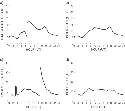
Figure 1. IONOLAB-TEC estimates for mate: before the cycle slip correction and interpo-lation (a) 29 March 2009 and (c) 6 April 2009; after cycle slip correction and interpointerpo-lation (b) 29 March 2009 and (d) 6 April 2009.
TEC estimates have been compared to Global Iono-spheric Map (GIM) TEC from various International GPS Service (IGS) stations [International GPSS Service, 2013] and empirical ionospheric models in Arikan et al. [2007], and it is shown that Reg-Est TEC estimates are in accordance with IGS TEC, especially with those from Jet Propulsion Laboratory (JPL) and Center for Orbit Determination in Europe (CODE), University of Bern. In Nayir et al. [2007], the effect of ionospheric peak height, choice of weighting function and inclusion of satellite and receiver bias to GPS-TEC computational model are investigated for Reg-Est. In Arikan et al. [2008], the method for determining receiver inter-frequency bias for a single GPS station, namely IONOLAB-BIAS, is introduced.
[6] Since 2007, modified Reg-Est that uses
IONOLAB-BIAS has been programmed in JAVA and started to be used as a trial version of automatic, online TEC estima-tion routine on www.ionolab.org as detailed in [Ugurlu, 2007; Ugurlu et al., 2007]. This service has been utilized by various researchers and TEC estimates are cited and/or utilized in studies including but not limited to TEC modeling/prediction [Sibanda, 2010; Ercha et al., 2012; Ackermann et al., 2011; Hernández-Pajares et al., 2011],
space-time interpolation (mapping) [Yilmaz et al., 2009; Foster and Evans, 2008; Jin and Jin, 2011], Computerized Ionospheric Tomography [Erturk et al., 2009; Sibanda, 2010; Jin and Jin, 2011; Hirooka et al., 2012], seismic precursor research from ionosphere [Karatay et al., 2010; Arikan et al., 2012; Contadakis et al., 2012; Hirooka et al., 2012], and TEC vari-ability and within-the-hour statistics [Erol and Arikan, 2005; Turel and Arikan, 2010; Sayin et al., 2010; Li et al., 2010; Rao et al., 2010; Maltseva and Mozhaeva, 2011]. With the grants from The Scientific and Technological Research Council of Turkey (TUBITAK), the Reg-Est with IONOLAB-BIAS has been further developed into an automatic, online, near-real time space weather application that is called IONOLAB-TEC.
[7] In this paper, the technical details of
IONOLAB-TEC estimation and the online, near-real time applica-tion to any IGS or EUREF staapplica-tion as a space weather service are provided. To our best knowledge, this service is original and unique as a space weather application. Section 2, includes a brief discussion on automatic prepro-cessing stages, Reg-Est computation, and bias estimation of IONOLAB-TEC. The emphasis will be on near-real time TEC computation. In section 3, the web application is introduced and example outputs are provided.
0 2 4 6 8 10 12 14 16 18 20 22 24 0 10 20 30 40 HOUR (UT) IONOLAB−TEC (TECU) 0 2 4 6 8 10 12 14 16 18 20 22 24 0 10 20 30 40 HOUR (UT) IONOLAB−TEC (TECU) 0 2 4 6 8 10 12 14 16 18 20 22 24 0 10 20 30 40 50 60 70 80 HOUR (UT) IONOLAB−TEC (TECU) 0 2 4 6 8 10 12 14 16 18 20 22 24 0 5 10 15 20 25 30 HOUR (UT) IONOLAB−TEC (TECU) c) d)
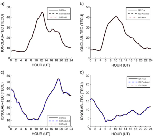
Figure 2. The effect of using different ephemerides files in IONOLAB-TEC on 7 March 2012: IGS rapid (dotted line), predicted (dashed line) and final (solid line); (a) ebre, (b) dear, (c) bogt, (d) palm.
2. Brief Overview of IONOLAB-TEC
[8] Estimation of TEC from a single GPS receiver
recordings in Receiver Independent Exchange (RINEX) format requires three major steps: First step is the pre-processing of data to be used in TEC computation; second step is the computation of TEC; third step is presenta-tion of data in a format that can be easily used by other researchers. In the following, these steps will be outlined for online, near-real time, and automatic computation of IONOLAB-TEC.
2.1. Preprocessing Stage of RINEX Data
[9] The RINEX files for the IGS/EUREF stations are
usually uploaded with a one day latency. Once the RINEX file for the desired IGS/EUREF station(s) is(are) available in the archive sites such as “ftp://igs.ensg.ign.
fr/pub/igs/data/,” “http://garner.ucsd.edu/pub/rinex/,”
“ftp://gnss1.tudelft.nl/rinex/,” and “ftp://geodaf.mt.asi.it/ GEOD/GPSD/RINEX/,” it is downloaded to IONOLAB server at Hacettepe University, Ankara, Turkey. Then, the following steps are taken for the preprocessing of RINEX and preparation of necessary parameters:
[10] 1. For a desired date (or dates) and desired
IGS/EUREF station(s), the RINEX file(s) is(are) down-loaded and the recorded pseudorange and phase delay information for every 30 s and for each satellite are extracted from this RINEX file. The coordinates of receiver station in the RINEX file are extracted. The coordinates of IGS and EUREF stations are also collected in a database file within the server. If for any reason, the RINEX file does not include the position of the receiver, then a search in the database for receiver coordinates is conducted by the program. Thus, the program will continue to run in both cases.
[11] 2. The satellite ephemerides data (http://igscb.
jpl.nasa.gov/components/prods.html) is accessed at the sites “ftp://garner.ucsd.edu/pub/products/,” “ftp://cddis. gsfc.nasa.gov/pub/gps/products/,” or “ftp://igscb.jpl.nasa. gov/pub/product/.” The available files for satellite posi-tions are broadcast, ultra rapid, rapid, and final. The latency on these different ephemerides data varies from real-time as in broadcast and predicted half of ultra rapid with a sampling interval of 15 min, 3–9 h in observed half of ultra rapid with a sampling interval of 15 min, 17–41 h for rapid with a sampling interval of 15 min, and 12–18 days for final also with a sampling interval
0 2 4 6 8 10 12 14 16 18 20 22 24 0 10 20 30 40 50 HOUR (UT) IONOLAB−TEC (TECU) IONOLAB−TEC (TECU) a) 0 2 4 6 8 10 12 14 16 18 20 22 24 0 10 20 30 40 50 HOUR (UT) IONOLAB−TEC (TECU) b) 0 2 4 6 8 10 12 14 16 18 20 22 24 0 10 20 30 40 50 60 70 80 HOUR (UT) c) 0 2 4 6 8 10 12 14 16 18 20 22 24 0 5 10 15 20 25 30 HOUR (UT) IONOLAB−TEC (TECU) d)
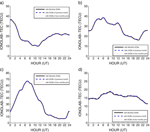
Figure 3. The effect of using different satellite bias (DCBs) values in IONOLAB-TEC on 17 May 2012: monthly satellite bias (solid line), satellite bias values of previous month (dashed line), and satellite bias values for two months prior (dotted line); (a) amc2, (b) bjfs, (c) bako, (d) joen.
of 15 min. IONOLAB-TEC routine checks the availability of ephemerides files and downloads the latest file. Since RINEX file provides data for every 30 s, an interpolation is performed on satellite positions to increase the sampling interval to 30 s. The satellite position information is used in computation of local elevation and azimuth angles.
[12] 3. With a novel automatic routine developed in
IONOLAB, the health of the recorded pseudorange and phase delay values are checked, and Cycle Slips are corrected as described in Sezen and Arikan [2012] using the original algorithm developed in IONOLAB. Phase delay recordings are leveled onto pseudorange values for com-putation of baselines and extraction of phase ambiguity as explained in detail in Nayir et al. [2007].
[13] 4. The automatic routine accesses to IGS
anal-ysis center site “ftp://cddis.gsfc.nasa.gov/gps/products/ ionex/” and downloads the available IONEX maps includ-ing the satellite bias values with a temporal resolution
of 2 h and spatial resolution of 5ı in longitude and 2.5ı
in latitude. These files are either in the form of “rapid ionospheric TEC grid” (with a latency of less than 24 h and the accuracy of data is between 2 to 9 TECU) or “final ionospheric TEC grid” (with a latency of approximately 11 days and the accuracy of data is between 2 to 8 TECU).
Satellite bias data may also be presented with a delay of 10 days up to a month. If the IGS analysis center site does not contain the satellite bias data for the desired day, the automatic IONOLAB routine searches for the nearest day data that has the satellite bias values.
[14] 5. The IONEX data is used in IONOLAB-BIAS
routine for computation of inter-frequency receiver bias as detailed in Arikan et al. [2008].
2.2. Computation of IONOLAB-TEC
[15] IONOLAB-TEC values are estimated from
prepro-cessed RINEX files [Komjathy, 1997; Schaer, 1999] using the satellite and receiver bias values, and receiver and satellite locations as follows:
[16] 1. The total number of electrons on a ray path is
called as Slant TEC (STEC). Using the inter-frequency satellite bias, IONOLAB-BIAS inter-frequency receiver bias, and pseudorange-leveled baseline phase delay values in the model provided in Nayir et al. [2007], STEC for every satellite is computed with 30 s time resolution (IONOLAB-STEC).
[17] 2. The total number of electrons in the local zenith
direction is called Vertical TEC (VTEC). VTEC can be obtained from STEC by the use of a “mapping function”
0 2 4 6 8 10 12 14 16 18 20 22 24 0 10 20 30 40 HOUR (UT) IONOLAB−TEC (TECU) 0 2 4 6 8 10 12 14 16 18 20 22 24 0 10 20 30 40 HOUR (UT) IONOLAB−TEC (TECU) 0 2 4 6 8 10 12 14 16 18 20 22 24 0 10 20 30 40 50 60 70 80 HOUR (UT) IONOLAB−TEC (TECU) c) 0 2 4 6 8 10 12 14 16 18 20 22 24 0 5 10 15 20 25 30 HOUR (UT) IONOLAB−TEC (TECU) d)
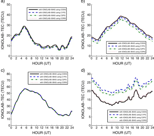
Figure 4. The effect of using different IONEX maps in IONOLAB-BIAS computation on 6 August 2011: codg (solid line), c1pg (dashed line), c2pg (dash dotted line), and corg (dotted line); (a) cedu, (b) tubi, (c) ntus, (d) reso.
as explained in Arikan et al. [2003]; Schaer [1999]; Komjathy [1997]. STEC is converted into IONOLAB-VTEC by the application of the mapping function provided in Arikan et al. [2003]; Nayir et al. [2007] for every position of the satellite with a 30 s time resolution.
[18] 3. By combining the VTEC for each satellite in the
least square sense by employing a weighting function to
reduce the multipath effects with an elevation mask of 30ı,
Reg-Est algorithm is applied to obtain TEC estimates in the form of IONOLAB-TEC with 30 s time resolution as discussed in Arikan et al., [2003; 2004]; Nayir et al., [2007]. If there is a data discontinuity in IONOLAB-TEC estimates due to gaps in RINEX file, an interpolation routine based on C-Spline is applied to the data gap, which is less than 15 min duration and if the magnitude of the difference of IONOLAB-TEC values at the end points of the gap is less than 3 TECU as described in [Sezen and Arikan, 2012]. 2.3. Presentation of IONOLAB-TEC
[19] IONOLAB-TEC estimates can be obtained for
one IGS/EUREF station, for more than one IGS/EUREF stations, for 1 day, or for more than 1 day. Compar-isons with Center for Orbit Determination in Europe (CODE), University of Bern, Switzerland, European Space
Operations Center of European Space Agency (ESA/ ESOC) Darmstadt, Germany, Jet Propulsion Laboratory (JPL) Pasadena, California, USA (JPL-GNISD), group of Astronomy and Geomatics, Universitat Politecnica de Catalunya, (gAGE/UPC) Barcelona, Spain, the weighted combination of VTEC estimates from CODE, ESA, JPL, and UPC (IGS), the hourly maps of gAGE/UPC (gAGE/ UPC-H), CODE Rapid, CODE Predict-1day, and CODE Predict-2day estimates can be obtained. IONOLAB-TEC values can be presented in
[20] 1. a graphical form and comparisons with IGS
Analysis Center estimates of TEC, or
[21] 2. an excel file with 2.5 min time resolution. If
there is a demand for 30 s time resolution estimates, they can be provided for the desired day and date from www. ionolab.org.
2.4. Examples of Near Real-Time IONOLAB-TEC Computation
[22] The importance of the correction of cycle slips and
interpolation of data loss for short durations are demon-strated with an example case in Figure 1. In Figures 1a and 1c, the IONOLAB-TEC values before the cycle slip cor-rection and interpolation are provided for 29 March 2009
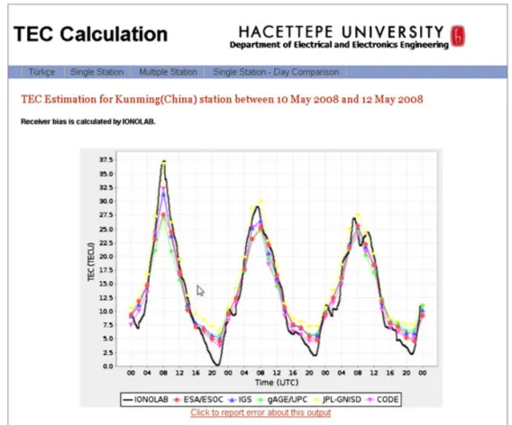
Figure 5. The screen capture of TEC computation for single station option for kunm from 10 to 12 May 2008.
and 6 April 2009, respectively, for IGS station mate (Italy). With the application of the novel cycle slip and interpola-tion algorithms, the reliability and accuracy of IONOLAB-TEC estimates are significantly improved as shown in Figures 1b and 1d for 29 March 2009 and 6 April 2009, respectively.
[23] In Figure 2, the effect of using different
ephemerides files, namely IGS rapid (dotted line), predicted (dashed line) and final (solid line), are inves-tigated for four different GPS stations on 7 March 2012. The seventh of March 2012 is the peak day of a severe geomagnetic storm on IZMIRAN Space Weather
Web-site (http://www.izmiran.ru/ionosphere/weather/storm/
tecstorm.txt) where Dst index decreased to –83 nT at 1600 UT (http://wdc.kugi.kyoto-u.ac.jp/dstdir/index.html) and Kp index increased to 6 (http://wdc.kugi.kyoto-u.ac. jp/kp/index.html) according to World Data Center for Geomagnetism (WDC) of Kyoto University, Japan. The IONOLAB-TEC values that are calculated using different IGS ephemerides data are presented for ebre (Spain, a midlatitude station) in Figure 2a, for dear (South Africa, a midlatitude station) in Figure 2b, for bogt (Colombia, an equatorial station) in Figure 2c, and finally, for palm (Antarctica, a high-latitude station) on 7 March 2012. As it can be observed from Figure 2, near real-time
IONOLAB-TEC computation with predicted or rapid ephemerides values is very robust and provides reliable estimates even for a stormy day, for stations in midlatitude, equatorial, and high-latitude regions.
[24] In Figure 3, the effect of using different satellite
bias (DCBs) values, namely monthly satellite bias (solid line), satellite bias values of previous month (dashed line), and satellite bias values for two months prior (dot-ted line) are investiga(dot-ted for four different GPS sta-tions on 17 May 2012. The 17th of May 2012 is the first Ground Level Enhancement (GLE) event of cycle 24 fol-lowing the Coronal Mass Ejection (CME) that occurred on the same day [Gopalswamy, 2012]. There is a fluctu-ation in both Dst and Kp indices on 17 May 2012. The IONOLAB-TEC values that are calculated using differ-ent satellite bias values are presdiffer-ented for amc2 (USA, a midlatitude station) in Figure 3a, for bjfs (China, a midlatitude station) in Figure 3b, for bako (Indonesia, an equatorial station) in Figure 3c, and finally, for joen (Finland, a high-latitude station) on 17 May 2012. As it can be observed from Figure 3, near real-time IONOLAB-TEC computation with different values of satellite bias values is very robust and provides reliable estimates even for a stormy day, for stations in midlatitude, equatorial, and high-latitude regions.
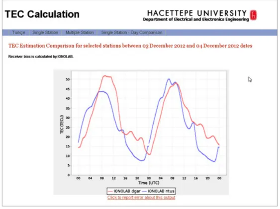
Figure 6. The screen capture of TEC computation for multiple station option for dgar and ntus from 3 to 4 December 2012.
[25] In Figure 4, the effect of using different IONEX
maps in IONOLAB-BIAS computation are investigated for four different GPS stations on 6 August 2011. IONOLAB-TEC values with IONOLAB-BIAS calculated using codg (CODE final) maps are indicated with a solid line, using c1pg (CODE one day predicted) maps are indicated with a dashed line, using c2pg (CODE two day predicted) maps are indicated with a dash dotted line, and corg (CODE daily) maps are indicated with a dotted line. On 6 August 2011, a very severe geomagnetic storm took place as given in IZMIRAN Space Weather Web site and WDC. Dst index decreased below –100 nT and Kp index increased to 8. The IONOLAB-TEC values that are calculated using IONOLAB-BIAS estimates obtained from codg, c1pg, c2pg and corg maps are presented for cedu (Australia, a midlat-itude station) in Figure 4a, for tubi (Turkey, a midlatmidlat-itude station) in Figure 4b, for ntus (Singapore, an equatorial station) in Figure 4c, and finally, for reso (Canada, a high-latitude station) on 6 August 2011. As it can be observed from Figure 4, near real-time IONOLAB-TEC computa-tion with different IONOLAB-BIAS estimates with final, daily and predicted maps is very robust and provides reliable estimates even for a stormy day, for stations in midlatitude and equatorial regions. The c1pg and c2pg maps were not able to predict the geomagnetic storm, therefore, there is a difference of 5 to 7 TECU between IONOLAB-TEC values that incorporated the effect of the storm in corg and codg maps of CODE.
3. Online Service for IONOLAB-TEC
[26] Near real-time, online service for automatic
IONOLAB-TEC computation is available on the site www. ionolab.org. The site is supported both in English and in Turkish. The first time users must register and further usage requires a username and password. Once member login with registered username and password is accom-plished, the user should click on the “IONOLAB-TEC Service” sign. There are three options for IONOLAB-TEC computation:
3.1. Single Station TEC Computation
[27] In the Single Station TEC Computation option, the
user is asked to enter the code of the IGS or EUREF station. If the station is on the map of IGS tracking network, then the map near the entry line can be called and by clicking on the station, the code can be entered automat-ically. The second entry is for the observation date. A duration of three consecutive days can be chosen either by the calender provided online and by clicking on the desired day, directly by typing the date day-month-year format into the box. “Show IONEX data” option box can be clicked if the user wants to observe the TEC estimates that are extracted from the IONEX maps of IGS analysis centers. “Output Type” option provides either an excel file output that can be opened or saved to the choice directory of the user, or a graphics option that provides a visual plot
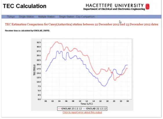
Figure 7. The screen capture of TEC computation for single station-day comparison option for cas1 from 22 to 23 December 2012.
of the available data. The computation takes action after the clicking of “Calculate” button. An example output is provided in Figure 5 for station kunm (Kunming, China), which is located 660 km south of the epicenter of the earth-quake that occurred on 12 May 2008. The plot indicates the IONOLAB-TEC along with the TEC estimates of IGS centers starting from 10 to 12 May 2008.
3.2. Multiple Station TEC Computation
[28] In the multiple station option, IGS and EUREF
stations can be added to the list using station code but-ton. The other options for observation start and end dates, IONEX data plot and output presentation in excel file or graphics are the same as single station case. In order to improve readability of the figures, the program can input up to three stations at a time. An example is provided in Figure 6 for two equatorial stations, namely dgar (Diego Garcia Island, USA) and ntus (National Technical Uni-versity of Singapore) for 3 to 4 December 2012, that has a mild to moderate disturbance in ionosphere and plas-masphere according to IZMIRAN Ionospheric Weather Web site, Wp disturbance index (http://www.izmiran.ru/ services/iweather/datw/wptec12.txt). The receiver bias is calculated using IONOLAB-BIAS using the latest update of IONEX maps. It is interesting to observe the effect of mild disturbance mostly during and after sunset hours. Here the IONEX output option is not chosen.
3.3. Single Station-Day Comparison TEC Computation
[29] In the single station-day comparison option,
non-consecutive days can be chosen to observe the variability between different dates for the same station up to 3 days. In Figure 7, a high-latitude station cas1 (Casey, Antarctica) is chosen for 22 and 23 December 2012. When the plot for Figure 7 was prepared, the final ephemerides, IONEX files were not available. Therefore, the screen capture indicates this by a note to the user that in calculation of receiver bias, rapid files are utilized. Also, the problem in phase delay recordings is resolved without disrupting the computa-tion. In this case, more noisy pseudorange recordings are utilized instead of phase delay. Due to the mild positive disturbance on 22 and 23 December 2012, the two con-secutive days are very different in peak values and TEC distribution with respect to hours in a day.
[30] If the excel file option is chosen, then the online
program asks the user in which directory the excel file should be saved. The name of the excel file can also be modified by the user at this stage. The first line of excel file contains the station(s) name(s) and date(s) of computation. Starting with A3 column, the date(s) of computation is(are) provided. The time of computation with 2.5 min resolu-tion is given in the column starting with B3. In order to reduce the online computation, the time resolution is kept at 2.5 min. If higher sampling rate is required, a 30 s time resolution can be provided on demand. Starting with C3,
all options listed above. The degree of decimal accuracy is for the user to choose.
4. Conclusion
[31] TEC is one of the most important observable
parameters of ionosphere. Monitoring of TEC provides a direct link to space weather events and understand-ing of the complex phenomena that takes place in near earth environment. In this study, the near real-time, online computation TEC is provided through the accurate and reliable Reg-Est algorithm under the name of IONOLAB-TEC from the Web site www.ionolab.org. After logging into the Web site, the user can choose to compute TEC for a single station, for a number of stations, for 1 day or for three consecutive days. Comparison of TEC for the same station and a number of different days is also available. An estimate of IONOLAB-TEC is provided as long as RINEX files are uploaded to the data centers. The IONOLAB-TEC algorithm is very robust to variations in the available IONEX, satellite bias and ephemerides files.
[32] Acknowledgments. This study is supported by TUBITAK EEEAG grants 105E171, 109E055, and 110E296. The authors wish to express their thanks to L. Lanzerotti of NJIT, M.E Contadakis of Aristotle University of Thessaloniki, and one other anonymous reviewer for their careful revision and insightful comments for the improvement of the manuscript.
References
Ackermann, E. R., J. P. de Villiers, and P. J. Cilliers (2011), Nonlinear dynamic systems modeling using Gaussian processes: Predicting ionospheric total electron content over South Africa, J. Geophys. Res., 116, A10303, doi:10.1029/2010JA016375.
Arikan, F., C. B. Erol, and O. Arikan (2003), Regularized estimation of vertical total electron content from Global Positioning System data, J. Geophys. Res., 108(A12), 1469, doi:10.1029/2002JA009605.
Arikan, F., C. B. Erol, and O. Arikan (2004), Regularized estimation of VTEC from GPS data for a desired time period, Radio Sci., 39, RS6012, doi:10.1029/2004RS003061.
Arikan, F., O. Arikan, and C. B. Erol (2007), Regularized esti-mation of TEC from GPS data for certain midlatitude stations and comparison with the IRI model, Adv. Space Res., 39, 867, doi:10.1016/j.asr.2007.01.082.
Arikan, F., H. Nayir, U. Sezen, and O. Arikan (2008), Estimation of single station interfrequency receiver bias using GPS-TEC, Radio Sci., 43, RS4004, doi:10.1029/2007RS003785.
Arikan, F., M. N. Deviren, O. Lenk, U. Sezen, and O. Arikan (2012), Observed ionospheric effects of 23 October 2011 Van, Turkey earthquake, Geomatics, Nat. Hazard. Risk, 3, 1–8, doi:10.1080/ 19475705.2011.638027.
Contadakis, M. E., D. N. Arabelos, C. Pikridas, and S. D. Spatalas (2012), Total electron content variations over southern Europe before and during the M 6.3 Abruzzo earthquake of April 6, 2009, Ann. Geophys., Special Issue: Earthquake Precursors, 55, 1.
Coster, A. J., E. M. Gaposchkin, and L. E. Thornton (1992), Real-Time ionospheric monitoring system using the GPS, Tech. Rep. 954, Lincoln Laboratory, Lexington, MA.
Ercha, A., D. Zhang, A. J. Ridley, Z. Xiao, and Y. Hao (2012), A global model: Empirical orthogonal function analysis of total electron content 1999–2009 data, J. Geophys. Res., 117, A03328, doi:10.1029/2011JA017238.
Erol, C. B., and F. Arikan (2005), Statistical analysis of the iono-sphere using GPS signals, J. Electromagn. Waves Appl., 19, 373–387, doi:10.1163/1569393054139615.
time, Adv. Space Res., 43, 1702–1710, doi:10.1016/j.asr.2008.08.018. Foster, M. P., and A. N. Evans (2008), An evaluation of interpolation
techniques for reconstructing ionospheric TEC maps, IEEE Trans. Geosci. Remote Sens., 46, 2153–2163, doi:10.1109/TGRS.2008.916642. Gopalswamy, N. (2012), A tell-tale sign of a wimpy solar cycle: The
first GLE event of solar cycle 24, IAU 28th General Assembly, Beijing, China, 20-31 August, 2012.
Hajj, G. A., L. C. Lee, X. Pi, L. J. Romans, W. S. Schreiner, P. R. Straus, and C. Wang (2000), COSMIC GPS ionospheric sensing and space weather, TAO, 11, 235–272.
Hernández-Pajares, M., J. M. Juan, J. Sanz, A. Aragon-Angel, A. Garcia-Rigo, D. Salazar, and M. Escudero (2011), The iono-sphere: Effects, GPS modeling and the benefits for space geodetic techniques, J. Geod., 85, 887–907, doi:10.1007/s00190-011-0508-5. Hirooka, S., K. Hattori, M. Nishihashi, S. Kon, and T. Takeda (2012),
Development of ionospheric tomography using Neural Network and its application to the 2007 Southern Sumatra earthquake, Electr. Eng. Japan, 181, pp. 9–18, doi:10.1002/eej.22298.
International GNSS Service (2013), http://igscb.jpl.nasa.gov/, [Accessed on January, 2013].
Jin, S., and R. Jin (2011), GPS ionospheric mapping and tomog-raphy: A case of study in a geomagnetic storm, IEEE Geoscience and Remote Sensing Symposium (IGARSS) 2011, 24-29 July 2011, Vancouver, Canada, 1127–1130.
Li, L., S. Zhang, Q. Hu, and J. Zhang (2010), Using IGS data to analyze the long-term variations of total electron content, IEEE 2nd Inter-national Conference on Information Engineering and Computer Science (ICIECS), 25-26 December 2010, 1–4.
Karatay, S., F. Arikan, and O. Arikan (2010), Investigation of total electron content variability due to seismic and geomag-netic disturbances in the ionosphere, Radio Sci., 45, RS5012, doi:10.1029/2009RS004313.
Komjathy, A. (1997), Global ionospheric total electron content map-ping using the global positioning system, Ph.D. dissertation, Department of Geodesy and Geomatics Engineering, University of New Brunswick, Fredericton, New Brunswick, Canada.
Maltseva, O. A., and N. S. Mozhaeva (2011), Features of short wave propagation in winter conditions, IEEE Proceedings of the 5th Euro-pean Conference on Antennas and Propagation (EUCAP), 11–15 April 2011, 1702–1705.
Nayir, H., F. Arikan, O. Arikan, and C. B. Erol (2007), Total elec-tron content estimation with Reg-Est, J. Geophys. Res., 112, A11313, doi:10.1029/2007JA012459.
Rao, N. V., T. Madhu, and K. L. Kishore (2010), Geomagnetic storm effects on GPS aided navigation over low latitude South Indian region, IJCSNS Int. J. Comput. Sci. Network Secur., 10, 37–42.
Sayin, I., F. Arikan, and K. E. Akdogan (2010), Optimum temporal update periods for regional ionosphere monitoring, Radio Sci., 45, RS6018, doi:10.1029/2009RS004316.
Schaer, S. (1999), Mapping and predicting the Earth’s ionosphere using the global positioning system, Ph.D. dissertation, University of Bern, Astronomical Institute.
Sezen, U., and F. Arikan (2012), A novel algorithm for cycle slip detection and repair, Geophys. Res. Abstr., 14, EGU2012-7586, EGU General Assembly 2012.
Sibanda, P. (2010), Challenges in topside ionospheric modelling over South Africa, Ph.D. dissertation, Rhodes University, South Africa. Steigenberger, P., M. Rothacher, R. Dietrich, M. Fritsche, A. Rülke,
and S. Vey (2006), Processing of a global GPS network, J. Geophys. Res., 111, B05402, doi:10.1029/2005JB003747.
Turel, N., and F. Arikan (2010), Probability density function estimation for characterizing hourly variability of ionospheric total electron content, Radio Sci., 45, RS6016, doi:10.1029/2009RS004345.
Ugurlu, O. (2007), Web based computation and presentation of Total Electron Content (TEC) using the IONOLAB method, (in Turkish with abstract in English) MS Dissertation, Hacettepe University, Ankara, Turkey.
Ugurlu, O., U. Sezen, and A. Z. Alkar (2007), Web based automated total electron content computation, Proceedings of RAST-2007, Recent Advances in Space Research, Harbiye, Istanbul, Turkey.
Yilmaz, A., K. E. Akdogan, and M. Gurun (2009), Regional TEC mapping using neural networks, Radio Sci., 44, RS3007, doi:10.1029/2008RS004049.