Integrated scheduling of production and logistics operations of a multi-plant manifacturer serving a single customer area

(1)

INTEGRATED SCHEDULING OF PRODUCTION AND

LOGISTICS OPERATIONS OF A MULTI-PLANT

MANUFACTURER SERVING A SINGLE CUSTOMER AREA

A THESIS

SUBMITTED TO THE DEPARTMENT OF INDUSTRIAL ENGINEERING

AND THE INSTITUTE OF ENGINEERING AND SCIENCE

OF BILKENT UNIVERSITY

IN PARTIAL FULFILLMENT OF THE REQUIREMENTS

FOR THE DEGREE OF

MASTER OF SCIENCE

By Merve Çelen

(2)

I certify that I have read this thesis and that in my opinion it is fully adequate, in scope and in quality, as a thesis for the degree of Master of Science.

___________________________________ Asst. Prof. Dr. Mehmet Rüştü Taner (Advisor)

______________________________________ Assoc. Prof. Dr. Oya Ekin Karaşan

______________________________________ Asst. Prof. Dr. Sedef Meral

Approved for the Institute of Engineering and Science ____________________________________

Prof. Dr. Mehmet Baray

(3)

ABSTRACT

INTEGRATED SCHEDULING OF PRODUCTION AND LOGISTICS

OPERATIONS OF A MULTI-PLANT MANUFACTURER SERVING A

SINGLE CUSTOMER AREA

Merve Çelen

M.S. in Industrial Engineering

Supervisor: Asst. Prof. Dr. Mehmet Rüştü Taner July, 2009

Increasing market competition forces manufacturers to continuously reduce their leadtimes by minimizing the total time spent in both production and distribution. Some studies in the relevant literature indicate that scheduling production and logistics operations in a coordinated manner leads to improved results. This thesis studies the problem of scheduling production and distribution operations of a manufacturer serving a single customer area from multiple identical production plants dispersed at different geographical locations. The products are transported to the customer area by a single capacitated truck. The setting is inspired by the operations of a leading soft drink manufacturer, and the objective is set in line with their needs as the minimization of the total completion time of the jobs. The completion time of a job is defined as the time it reaches at the customer area. We consider both this general problem and four special cases motivated by common practical applications. We prove that both the main problem and three of its special cases are NP-hard at least in the ordinary sense. We develop mixed integer programming (MIP) models for all these problems and propose a pseudo-polynomial dynamic programming mechanism for the remaining special case. Since the MIP models are able to provide optimal solutions only for small instances in a reasonable amount of time, heuristics are also proposed to solve larger instances. Fast lower bounds are developed to facilitate the performance assessment of these heuristics in medium and large instances. Evidence from extensive computational experimentation suggests that the proposed heuristics are both efficient and effective.

(4)

ÖZET

TEK MÜŞTERİ BÖLGESİNE HİZMET VEREN ÇOK TESİSLİ BİR

İMALATÇININ ÜRETİM ÇİZELGELEME VE LOJİSTİK

FAALİYETLERİNİN BÜTÜNLEŞİK PLANLAMASI

Merve Çelen

Endüstri Mühendisliği, Yüksek Lisans Tez Yöneticisi: Yrd. Doç. Dr. Mehmet Rüştü Taner

Temmuz, 2009

Yükselen pazar rekabeti imalatçıları üretim ve dağıtımda geçen toplam süreyi en küçülterek tedarik sürelerini sürekli olarak azaltmaya zorlamaktadır. İlgili literatürdeki bazı çalışmalar üretim ve dağıtım işlemlerinin bağlantılı bir şekilde çizelgelenmesinin daha iyi sonuçlar verdiğini göstermektedir. Bu tezde farklı coğrafik yerseçimlerindeki özdeş tesislerden tek müşteri bölgesine hizmet veren bir imalatçının üretim ve dağıtım işlemlerinin çizelgelenmesi çalışılmaktadır. Ürünler müşteri bölgesine taşıma kapasitesi belirli bir araç tarafından taşınmaktadır. Problemin tanımı ileri gelen bir alkolsüz içecek imalatçısının çalışmalarından esinlenilmiş ve amaç fonksiyonu onların ihtiyaçlarıyla uyumlu olacak şekilde işlerin bitiş zamanlarının toplamının en küçültülmesi olarak belirlenmiştir. Bir işin bitiş zamanı o işin müşteri bölgesine ulaştığı zaman olarak tanımlanmıştır. Hem genel problem hem de onun pratik uygulamalarda sıklıkla karşılaşılan dört özel durumu ele alınmıştır. Hem esas problemin hem de onun üç özel durumunun NP-zor olduğu kanıtlanmıştır. Tüm bu problemler için karışık tamsayılı programlama (KTP) modelleri geliştirilmiş ve geri kalan özel durum için sözde-polinom bir dinamik programlama mekanizması önerilmiştir. KTP modelleri eniyi sonuçları makul sürelerde sadece küçük örnekler için verebildiğinden büyük örnekleri çözebilmek için sezgisel yöntemler önerilmiştir. Sezgisel yöntemlerin orta ve büyük

(5)

geliştirilmiştir. Yapılan kapsamlı deneyler önerilen sezgisel yöntemlerin verimli ve etkili olduğunu göstermiştir.

Anahtar sözcükler: Çok tesisli çizelgeleme, dağıtım, karmaşıklık, tamsayı programlama,

(6)

(7)

Acknowledgement

First, I would like to express profound gratitude to my advisor, Asst. Prof. Dr. Mehmet Rüştü Taner, for sharing his experience and knowledge with me. I would like to thank him especially for tolerating me when I was upset and nervous.

I am also grateful to Assoc. Prof. Dr. Oya Ekin Karaşan and Asst. Prof. Dr. Sedef Meral for accepting to read and review this thesis and for their invaluable suggestions.

I am as ever, especially indebted to my family, Tülün, Ender and Elif Çelen, for their endless love and support. Everyday on the phone they tried to calm me down and motivate me for hours. Whenever I had a break down, their motivations made me continue. Even when we were at different continents their love was always with me and I would not be able to finish this thesis without them.

I want to thank my roommates Hande Koçak and Çiğdem Ataseven for sharing the life with me for two years.

My sincere thanks go to my friends Bora Karaoğlu, Büşra Çelikkaya, Hayrettin Gürkök, Tuncer Erdoğan, Adnan Tula, Utku Guruşçu, İhsan Yanıkoğlu, Safa Onur Bingöl, Emre Uzun, Hatice Çalık, Sıtkı Gülten, Serdar Yıldız, İpek Şener, Sezgin Küçükçoban and Erkin Bahçeci.

(8)

Finally, I would like to express my special thanks to TÜBİTAK for the scholarship provided throughout this thesis study.

(9)

LIST OF FIGURES

2.1. Literature classification for fleet type... 19

2.2. Literature classification for machine/plant configuration and customer area properties . 20 3.1. A representation of plant locations and distances to the customer area ... 22

3.2. Gantt chart for the optimal solution of sample problem with 10 jobs and 3 plants... 27

5.1. Numerical results for Heuristic 1 for n=25, 40,55 where p_j∈

[ ]

1,11 ...83

[ ]

1,11 ...83

5.3. Numerical results for Heuristic 1 for n=10 where p_j∈

[

5,15

]

...85

[

5,15

]

...85

[

5,15

]

...86

[

5,15

]

...87

5.7. Numerical results for Heuristic 1 for n=10 where pj∈

[

25,35

]

...88

[

25,35

]

...88

[

25,35

]

...89

5.10. Numerical results for Heuristic 2 for n=25, 40,55 where pj∈

[

25,35

]

...89

[

1,35

]

...91

[

1,35

]

...92

[

1,35

]

...92

[

1,35

]

...93

(13)

[ ]

1,11 ...95

[ ]

1,11 ...96

[

5,15

]

...97

[

5,15

]

...97

[

5,15

]

...98

[

5,15

]

...98

[

25,35

]

...99

[

25,35

]

...100

[

25,35

]

...100

[

25,35

]

...101

[

1,35

]

...102

[

1,35

]

...103

[

1,35

]

...103

[

1,35

]

...104

[ ]

1,11 ...105

[ ]

1,11 ...106

[

5,15

]

...107

[

5,15

]

...108

(14)

[

25,35

]

...112

[

1,35

]

...113

[

1,35

]

...113

[

1,35

]

...114

[

1,35

]

...114

[ ]

1,11 ...116

[ ]

1,11 ...117

[

5,15

]

...118

[

5,15

]

...118

[

25,35

]

...121

[

1,35

]

...122

(15)

LIST OF TABLES

4.1. Sample calculation of completion times of the trips for Lower Bound 1... 49

4.2. Trip Completion Times and Number of Jobs Carried in Lower Bound 2... 57

4.3. Trip Completion Times for Lower Bound 3... 58

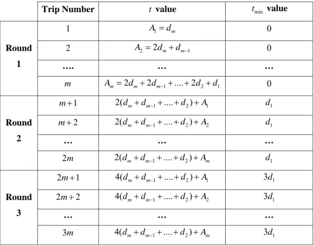
4.4. t and t_min calculation for Lower Bound 5... 72

5.1. Parameter settings for number of jobs and truck capacity ... 79

5.2. Parameter settings for processing times and plant distances... 81

5.3. LB and optimality gaps for Heuristics 1 and 2 for

(

n=25,K =8

)

and d_i∈

[

22, 28

]

...91

5.4. LB and optimality gaps for Heuristics 1 and 2 for

(

n=25,K =8

)

and d_i∈

[

22, 48

]

...91

5.5. LB and optimality gaps for Heuristic 5 and Heuristic 6 for n=10 and d_i∈

[

22, 28

]

...110

5.6. LB and optimality gaps for Heuristic 5 and Heuristic 6 for n=10 and di∈

[

32,38

]

....110

5.7. LB and optimality gaps for Heuristic 5 and Heuristic 6 for n=10 and d_i∈

[

22, 48

]

...111

5.8. LB and optimality gaps for Heuristic 7 for n=10 and d_i∈

[

22, 28

]

...119

5.9. LB and optimality gaps for Heuristic 7 for n=10 and di∈

[

32,38

]

...120

5.10. LB and optimality gaps for Heuristic 7 for n=10 and d_i∈

[

22, 48

]

...120

5.11. Performance assessment of the methods of special cases for the general problem... 125

C.1. Computational results for Last Trip Partial Problem where p_j∈

[ ]

1,11 and d_i∈

[

22, 28

]

...162

[ ]

1,11 and di∈

[

32,38

]

...166

(16)

[ ]

1,11 and d_i∈

[

22, 48

]

...170

[

5,15

]

and d_i∈

[

22, 28

]

...174

[

5,15

]

and d_i∈

[

32,38

]

...178

[

5,15

]

and d_i∈

[

22, 48

]

...182

[

25,35

]

and

[

22, 28

]

i

d ∈ ...186

[

25,35

]

and

[

32,38

]

i

d ∈ ...190

[

25,35

]

and

[

22, 48

]

i

d ∈ ...194

[

1,35

]

and

[

22, 28

]

i

d ∈ ...198

C.11. Computational results for Last Trip Partial Problem where pj∈

[

1,35

]

and

[

32,38

]

i

d ∈ ...202

[

1,35

]

and

[

22, 48

]

i

(17)

D.1. Computational results for Fully Loaded Trips Problem where p_j∈

[ ]

1,11 and

[

22, 28

]

i

d ∈ ...211

[ ]

1,11 and

[

32,38

]

i

d ∈ ...215

D.3. Computational results for Fully Loaded Trips Problem where pj∈

[ ]

1,11 and

[

22, 48

]

i

d ∈ ...219

D.4. Computational results for Fully Loaded Trips Problem where p_j∈

[

5,15

]

and

[

22, 28

]

i

d ∈ ...223

[

5,15

]

and

[

32,38

]

i

d ∈ ...227

[

5,15

]

and

[

22, 48

]

i

d ∈ ...231

[

25,35

]

and

[

22, 28

]

i

d ∈ ...235

[

25,35

]

and

[

32,38

]

i

d ∈ ...239

[

25,35

]

and

[

22, 48

]

i

d ∈ ...243

(18)

[

1,35

]

and

[

32,38

]

i

d ∈ ...251

[

1,35

]

and

[

22, 48

]

i d ∈ ...255

E.1. Computational results for No Wait Problem where pj∈

[ ]

1,11 and di∈

[

22, 28

]

...260

E.2. Computational results for No Wait Problem where p_j∈

[ ]

1,11 and d_i∈

[

32,38

]

...264

[ ]

1,11 and d_i∈

[

22, 48

]

...268

E.4. Computational results for No Wait Problem where pj∈

[

5,15

]

and di∈

[

22, 28

]

...272

[

5,15

]

and d_i∈

[

32,38

]

...276

[

5,15

]

and d_i∈

[

22, 48

]

...280

[

25,35

]

and d_i∈

[

22, 28

]

...284

[

25,35

]

and d_i∈

[

32,38

]

...288

[

25,35

]

and d_i∈

[

22, 48

]

...292

[

1,35

]

and d_i∈

[

22, 28

]

...296

[

1,35

]

and di∈

[

32,38

]

...300

[

1,35

]

and d_i∈

[

22, 48

]

...304

F.1. Computational results for General Problem where p_j∈

[ ]

1,11 and d_i∈

[

22, 28

]

...309

F.2. Computational results for General Problem where pj∈

[ ]

1,11 and di∈

[

32,38

]

...313

[ ]

1,11 and d_i∈

[

22, 48

]

...317

(19)

[

5,15

]

and d_i∈

[

32,38

]

...325

[

5,15

]

and d_i∈

[

22, 48

]

...329

[

25,35

]

and d_i∈

[

22, 28

]

...333

[

25,35

]

and d_i∈

[

32,38

]

...337

F.9. Computational results for General Problem where pj∈

[

25,35

]

and di∈

[

22, 48

]

...341

[

1,35

]

and d_i∈

[

22, 28

]

...345

[

1,35

]

and d_i∈

[

32,38

]

...349

(20)

Chapter 1

INTRODUCTION

The main focus of scheduling is the allocation of limited resources to tasks over time with the objective of optimizing with respect to one or more performance measures. Recent developments in scheduling have focused on extending various classical models to address real-life problems more closely. In today’s competitive business world, as the concept of on-time delivery of jobs has become more crucial for customer satisfaction, effective scheduling of production resources, achieving reduction in inventory levels and shortening lead times have gained much criticality.

Many studies in scheduling literature have concentrated on how to effectively schedule production operations within the confines of a single production facility. However, from the perspective of minimizing the total cost in a supply chain, companies usually acknowledge that the cost of a product is not only determined with the amount of factory resources used to convert the raw material into a finished product, but also with the amount of resources used to deliver the product to the customer. Hence, concentrating only on scheduling of production operations within plants may not be sufficient to obtain the desired low levels in the production and logistics costs of the supply chain. From another perspective to increase customer satisfaction, the order lead times should also be minimized. This requies the time spent both in the production of the product and in its distribution to be minimized

The importance of the coordination between production and distribution operations have been studied in Chandra and Fisher (1994), Ertogral et al. (1998), and Fumero and

(21)

Vercellis (1999). It has been shown that integrated scheduling of production and distribution operations perform substantially better than unsynchronized scheduling of these operations. Hence, it is important for the companies to recognize that a reduction in total cost of the supply chain and an increase in customer satisfaction can be realized through integrated scheduling of production and distribution operations.

In the relevant literature there have been various studies that concentrate on the integration of production and distribution operations. However, most of those studies have considered a single production plant with different machine configurations. To the best of our knowledge, there are only two studies in the relevant literature that try to address the problem with decentralized plant locations, the studies of Chen and Pundoor (2006) and Li and Ou (2007). In these works, the products have a very short selling season, and are transported from the plants to a warehouse via a third-party carrier and it is assumed that a transporter would be available at each facility whenever one is required. However, as experienced by a leading soft drink manufacturer in Turkey, third-party carriers may cause high distribution costs and long lead times. Because of increasing demand the prices of the trucks supplied by these third-party carriers are increasing while the availability of the trucks is decreasing. Therefore, aforementioned soft drink manufacturer has considered building its own fleet.

In order to address the problems faced by the soft drink manufacturer, in this thesis, we study the problem of integrated scheduling of production and distribution operations of a manufacturer with multiple production plants at different locations serving a single customer area via a single capacitated truck. Assuming that a truck is assigned to each warehouse and that truck is used to transport the products from the plants to that warehouse, our work can also be used to find a good solution for a larger system with decentralized plants and multiple warehouses.

As in the problem studied in Qi (2008), in order to satisfy unexpected customer demand on time, some companies may choose outsourcing from other plants at different

(22)

locations. Assuming that the outsourcing company has a single capacitated truck, proposed methods in this thesis can be used to address the problem of outsourcing.

The rest of this thesis is organized as follows. The next chapter gives a summary of the relevant literature in the area of integrated scheduling of production and distribution operations. Chapter 3 gives a precise explanation of the problem setting and necessary notations. In Chapter 4, dynamic programming algorithms for the problem where the assignments of the jobs to the plants are known are provided. In addition to that, heuristic and exact algorithms and lower bound generation methods for the three special cases and the original problem are explained in detail. Following that, in Chapter 5, the experimental design to test the performance of the proposed methods and the numerical results obtained in the generated test problems are given. A general conclusion of the study is presented in Chapter 6.

(23)

Chapter 2

LITERATURE REVIEW

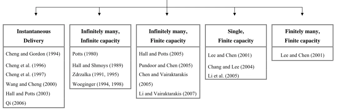
There are many studies in the literature which consider the integration of production and distribution operations. We study the problem with m identical plants at different locations serving a single customer area. We consider a single truck with finite capacity to transport the jobs from the plants to the customer area. To give the related literature, we will first review the papers according to their fleet types in the Section 2.1. Then in Section 2.2, we will continue with the review of the literature based on the machine configuration and customer area properties.

2.1. Studies with Different Fleet Types

The fleet types considered in the scheduling literature can mainly be grouped based on two aspects: the number of trucks in the fleet and the capacity of the trucks. Most of the studies up to date assume a fleet consisting of infinitely many trucks, a few of which integrate a capacity constraint for the trucks.

The first papers in scheduling research that focuses on problems where the completion time of a job is defined as the time the job reaches the customer, mainly consider a fleet of infinitely many trucks. They do not consider a capacity constraint for the trucks. Although this assumption of infinite capacity simplifies the problem, it is not realistic. Potts (1980), Hall and Shmoys (1989), Zdrzalka (1991, 1995) and Woeginger (1994, 1998) are the

(24)

first ones to use this assumption. They assume that whenever a job finishes its production, there is always a truck available to immediately deliver the job to the customer in q_j time

where q_j denotes the time required to transport job j from the machine/plant to the customer.

Hence the time a job reaches the customer is the process completion time of that job at the plant plus the transportation time of that job.

In the studies of Cheng et al. (1996), Cheng and Gordon (1994), Cheng et al. (1997) and Wang and Cheng (2000), the delivery time of a batch is defined as the completion time of the last job in that batch. Here, the transportation is assumed to be instantaneous. However, the objective functions to minimize contain a term for delivery cost and delivery cost depends on the number of deliveries made to transport all the jobs from the plant to the customer. Hall and Potts (2003) make the same instantaneous transportation assumption in their paper that studies scheduling problems in a supply chain where a supplier makes deliveries to several manufacturers. Also these manufacturers make deliveries to customers. Again in the study of Qi (2006), the transportation from the facility to the customer is assumed to be instantaneous. However, for the transportation between facilities at different locations, infinitely many trucks are used and a transshipment time is required.

The study of Hall and Potts (2005) also investigates the condition where there are infinitely many trucks. However, they also consider the case when there is only one truck. They combine these two different truck constraints by defining a parameter T which denotes the minimum time between any two consecutive deliveries. If there are a sufficient number of trucks, T is defined as the time it takes to load a truck; else if there is a single truck, it is defined as the travel time to and from the customers plus the loading time.

The papers of Pundoor and Chen (2005) and Chen and Vairaktarakis (2005) consider the case with a fleet of infinitely many trucks. However, their fleet choice is more realistic when compared with the aforementioned ones since they take the capacity constraint into account. In Chen and Vairaktarakis (2005), it is assumed that distribution operations are

(25)

carried out by third-party carriers and thus an unlimited number of vehicles are available. But due to limited vehicle capacity, each truck can carry up to a certain number of jobs. The same third-party carrier assumption with vehicle capacities also holds in the study of Li and Vairaktarakis (2007).

Chang and Lee (2004) study a more difficult problem by considering a single and capacitated truck. They define the completion time of a sequence as the time when the vehicle finishes delivering the last batch to the customer site(s) and returns to the machine(s). The reason for this definition is that to have a cyclic pattern they have to wait for the truck to return to the machine. An interesting point to mention about their study is that they assume each job might occupy a different amount of physical space in the truck. Li et al. (2005) also incorporate the same single and capacitated truck idea in their study. However, their capacity constraint is defined so that the truck can also behave as uncapacitated. They define the capacity of the truck to be K and they add that K can also be equal to the number of jobs, i.e.

n, which means an unlimited capacity.

Although it may seem that third-party carrier assumption is reasonable, it should also be taken into account that to decrease transportation cost, many manufacturing companies prefer to build their own fleet. Since the number of trucks in such a fleet will be limited, the assumption of infinitely many trucks becomes unreasonable. It is also for sure that for a more realistic assumption, each truck will have a capacity constraint. From this perspective, Lee and Chen (2001) can be considered as a milestone in the literature relevant to the integration of production and distribution. They study two classes of transportation: within the facility and from the facility to the customer. For both transportation classes, they consider various types of fleet. The types of fleet they assume in their study can be listed as follows:

• Single truck which can carry only one job at a time

• Single truck which can carry more than one but fewer than n jobs • Single truck which can carry n/2 jobs

(26)

• Multiple but limited number of trucks, each can carry more than one but fewer than n jobs

Although single truck case has been studied before, Lee and Chen (2001) is the first to consider multiple trucks.

As mentioned in Chapter 1 for the soft drink manufacturer, using third-party carriers may cause high distribution costs and long leadtimes. To reduce the distribution costs and leadtimes, it is a reasonable alternative for the companies to have their own fleet instead of using third-party carriers. It is logical for large companies to assign a truck to each of their warehouses and each warehouse would be responsible from using its own truck to have their products delivered to them from the plants. In this context, in our problem, having a single truck with a finite capacity is realistic. Also, for a small company which uses outsourcing from plants at different locations, having a single capacitated truck to gather the products from other plants is logical.

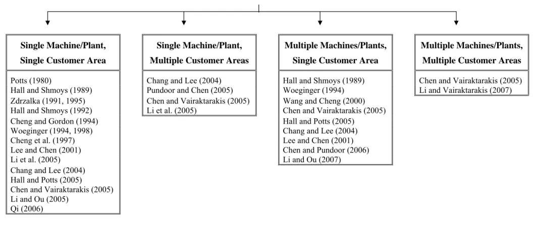
2.2. Studies with Different Machine Configuration and Customer

Area Properties

In the literature relevant to simultaneous scheduling of production and distribution, there have been various studies considering different types of machine configurations and different structures for the customer location, e.g.. a single customer area or multiple customer areas. For the machine configuration part, there are many papers that study single machine, parallel machines or a series of flow shop machines. So it would be beneficial to group the relevant literature according to their combinations of machine configuration and customer area. In such a case, four main groups may occur:

(27)

• Single machine and multiple customer areas • Multiple machines and single customer area • Multiple machines and multiple customer areas

We will review the studies in each group in the same order as they are stated above.

2.2.1. Single Machine and Single Customer Area

Most of the papers, especially the earliest ones, in the relevant literature consider this case in their studies. The reason for this is that single machine scheduling is relatively easier than multiple machine scheduling. Also sending the jobs to a single customer area eliminates routing issues and hence the problem becomes easier. Some of the papers in this area consider batching, which means that each batch will consist of a pre-specified amount of jobs. We will first review the studies which do not consider a batch concept as defined above.

The first paper that considers the scheduling of the production on a single machine and delivery of the finished products to a single customer is the study of Potts (1980). In his paper, Potts tries to find a sequence for the jobs, each of which has a release date (r ), a i nonnegative processing time (p ) and a delivery time (_i q ). The objective is to minimize the _i

time by which all jobs are delivered. One of the interesting points in this study is the

symmetric form of the original problem created by defining due dates for each job i by

assigning d = K - i qi where K is a constant. This forms a modified problem in which due dates replace the delivery times. Hence, minimizing the makespan in the symmetric form is equivalent to minimizing maximum lateness with respect to the due dates. This problem was shown to be NP-hard by Lenstra et al. (1977) and Potts develops a heuristic that is guaranteed to produce a solution within 50% of the optimum.

(28)

Hall and Shmoys (1989) also consider release times, processing times and delivery times for the jobs. With a similar modification of the problem as in Potts (1980), they convert the makespan problem into a maximum lateness problem. They denote the problem as

max

1r Lj using the notation of Graham et al. (1979) and they provide a polynomial time approximation scheme for this problem. For the special case, where r_j = 0, they use the

Jackson’s Rule to solve the problem optimally in polynomial time. They also investigate the case where precedence constraints between jobs are involved. They provide a (4/3)-approximation algorithm for1 , rj prec L_max. Hall and Shmoys (1992) give a detailed explanation of their (4/3)-approximation scheme and provide two polynomial approximation schemes for the problem1r L_j _max. Woeginger (1994) considers similar job properties but

with the exception that he does not take release times into account. For the single machine case, Woeginger modifies the problem as in Potts (1980) and transforms it into1 L_max. It is stated that sequencing the jobs in non-increasing delivery times, i.e. sequencing the jobs according to earliest due date rule, yields an optimum schedule in O(n log n) time. The author also claims that no algorithm that is asymptotically faster than O(n log n) can construct an optimum schedule for this problem.

Lee and Chen (2001) consider two different objectives in their study: minimizing the time by which the last job reaches the customer and minimizing the total flow time. The main importance of their study is that they assume a limited number of trucks with finite capacity and hence there is not a delivery time assigned to each job. In fact the delivery time for each job is determined by the distance of the machine to the customer. For the objective of minimizing the makespan, the paper shows that this single machine problem with multiple trucks can easily be converted to a parallel machine problem where each truck is treated as a machine. The modified problem is denoted as Pv r_j, p_j ≡ p C_max where v is the number of

trucks, p is the time to travel from the machine to the customer and turn back to the machine. It is stated that this problem can be solved optimally in polynomial time. For the total flow

(29)

time case, a polynomial time dynamic programming algorithm is presented. Later Li et al. (2005) present a more efficient dynamic programming algorithm for this case. Chang and Lee (2004) consider a similar problem but with a single truck condition. It is shown that minimizing the makespan subject to these constraints is NP-hard in the strong sense. The authors provide a heuristic for the problem which produces solutions with an error bound of 5/3.

Hall and Potts (2005) again study the single plant and single customer area setting with finitely many capacitated trucks, but also in order to minimize the number of trips required to deliver all the jobs, the authors include the transportation cost into their objective functions. Their study considers a constraint T, which denotes the minimum time interval between two consecutive deliveries which was explained in more detail in Section 2.1. For the problems1T Dy+

∑

Cj, 1 T Dy L+ max, and 1T Dy+

∑

Uj, where D denotes the delivery cost for each trip and y denotes the number of trips, polynomial time algorithms are provided to find an optimal schedule whereas for the problems 1T Dy+

∑

w Uj j and

1 Dy+

∑

T_j pseudopolynomial algorithms are presented. The study also shows that

recognition versions of problems 1 Dy+

∑

w Cj j and 1T Dy+

∑

w Cj j are unary NP-complete. Chen and Vairaktarakis (2005) also incorporate distribution cost into their objective functions but differently from Hall and Potts (2005) infinitely many capacitated trucks are considered. The objective is to minimize total distribution cost and mean (or maximum) delivery time simultaneously and polynomial time algorithms are provided for these problems.

In Li and Ou’s (2005) work, a single capacitated truck is used to carry unprocessed jobs from the warehouse to the plant and processed jobs from the plant to the warehouse. The study aims to minimize the makespan and polynomial time algorithms for some special cases and a heuristic for the general problem are proposed.

(30)

Although Qi (2006) considers two machines at different locations, since each machine serves to its own customer area, it is more suitable to review this study in this section. The reason for the authors to mention the locations of the plants is that whenever the demand in one of the processing facilities, named facility 1, exceeds its capacity the other facility’s, named facility 2, capacity may be used and the jobs processed there should be transferred to

facility 1 again. Then the jobs are delivered from facility 1 to its customer. Both batch

transshipment and item transshipment are considered under different objective functions and algorithms (mostly dynamic programming) are developed for them.

The notion of batching starts with Zdrzalka (1991). In this study, a unit setup time associated with switching from jobs in one batch to those in another is inserted. Three polynomial time heuristics so as to minimize the time by which the last batch reaches the customer are proposed. Zdrzalka (1995) generalizes the problem to sequence independent setup times and provides two approximation algorithms with the worst-case performance ratio of 3/2. In Woeginger (1998), a polynomial-time approximation scheme is provided for the problem in Zdrzalka (1995). In addition to that, it is shown that finding a polynomial-time approximation algorithm with constant worst-case ratio is not possible for a variant of the problem where sequence-dependent setup times are involved. Setup times are involved also in the study of Cheng et al. (1997). The authors assume that there is a constant setup time between two consecutive batches. The objective is to find a number B of batches and a sequence so as to minimize the sum of the total weighted job earliness and mean batch delivery time. They prove that the problem is NP-hard in the strong sense. It is stated that even for the case where the number of batches has a fixed upper bound, the problem is NP-hard in the ordinary sense and a dynamic programming algorithm which solves this problem in pseudopolynomial time is provided. For this upper bound case, it is shown that the complexity does not change even if the setup times are equal to zero. Also the authors prove when B has a fixed lower bound the problem remains strongly NP-hard. For the special cases where all the weights are equal or all the processing times are equal, polynomial time algorithms are derived. Finally, a heuristic approach is presented for the general problem.

(31)

Cheng and Gordon (1994) again consider the batching concept on a single machine scheduling environment. The objective is to minimize the total distribution cost that mainly depends on the number of batch deliveries. The authors provide a dynamic programming approach which yields two pseudopolynomial algorithms when the number of batches has a fixed upper bound. In this study the authors also consider a special case where the processing times of the jobs in the same batch are assumed to be equal. A polynomial algorithm for this special case is presented.

2.2.2. Single Machine and Multiple Customer Areas

There are not many studies that fall into this category. The main reason for this is that routing decisions may be involved when there are multiple customers at different locations.. Also the properties of the batches are again determined according to these routing decisions. Although we consider identical plants at different locations and a single customer area in our study, this case has considerable importance for our research. In order to get an intuition for our study, it is possible to think the reverse of this multiple customer areas case.

Considering multiple customer areas is a relatively new concept and the study of Chang and Lee (2004) is among the first papers in this area. Two customer areas are considered and the finished products are delivered with a single and capacitated vehicle allowing milkrun. The distances from the machine to each customer are prespecified. The objective is to minimize the time by which all the jobs reach their customers. All jobs delivered in one shipment are called as a batch and it is stated that if the assignment of the jobs to the batches is known, the problem can easily be converted to a two-machine flow shop problem with the objective of minimizing the makespan where the vehicle is seen as the second machine. For this special case Johnson’s rule solves the problem optimally. However, the original problem is shown to be NP-hard in the strong sense. A heuristic is provided that yields solutions with a worst case error bound of 7/4.

(32)

Pundoor and Chen (2005) consider the case with m customers positioned at different locations. It is assumed that only direct shipping from the supplier to the customer is used, i.e. no milkrun. Therefore, only the jobs associated to the same customer can be delivered together in a shipment. A combined objective function which considers both the maximum tardiness and the total distribution cost is used. It is shown that for arbitrary number of customers, the problem is NP-hard even for the special case where the processing times and due dates are agreeable (i.e. if pi ≤ pj then di ≤dj). A fast heuristic which is capable to generate near optimal solutions is provided. One of the most important properties of this study is that they have showed that using the integrated production-distribution approach is more advantageous when compared to the approach of optimizing production and distribution sequentially with little or no integration.

The study of Chen and Vairaktarakis (2005) is important as it considers all the machine configuration and customer area cases. In this section, we will only review the single machine and multiple customer case. They allow milkrun in their study and determine the distances of the customers to the processing facility according to the milkrun routes. Their objective is to minimize total distribution cost and mean (or maximum) delivery time simultaneously and they provide efficient dynamic programming algorithms to solve these problems optimally.

Li et al. (2005) is one of the studies we base our research on. This study considers m customers at different locations and aims to minimize the total flow time. First, the problem is proven to be NP-hard in the strong sense. For the case where milkrun is allowed, first a pseudopolynomial dynamic programming algorithm for two-customers is provided and then generalized to multiple customers. Another dynamic programming algorithm for the case with only direct shipments is presented. The authors conclude that the computational complexity is lowered when the deliveries are restricted to direct shipments.

(33)

2.2.3. Multiple Machines and Single Customer Area

This is the second most widely studied case after single machine and single customer area. In this section, we consider mainly two types of problems. The first type is with a single production plant that has different machine configurations such as parallel machines, flow shops, and job shops. The second type considers multiple production plants dispersed at different geographic points where each plant can be viewed as a single machine. The problem studied in this thesis is among the second type. In our research we consider m identical machines at different locations and a single customer area. Delivery to the customer can be made from all of the plants via a single truck with a certain capacity. To the best of our knowledge, no one has studied this problem before. In our problem only direct shipments are allowed. Most of the studies in the relevant literature consider direct shipments. The studies that consider milkruns will be mentioned both in this and the following section.

Most of the work issuing multiple machines and a single customer area address the problems where the machines are located at the same location, i.e. parallel or flow-shop machines. The studies with parallel machines can be regarded as special cases of our problem where the distances between the machines are negligible and products of different machines can be transported on the same shipment.

Hall and Shmoys (1989) consider two multiple machine problems in their study. In the first one, their objective is to minimize maximum lateness of jobs with respect to release dates and delivery times in a parallel machine environment. They provide a polynomial approximation scheme for the case without precedence constraints and a 2-approximation algorithm for the case considering precedence. A two-machine flow shop environment is considered for the second problem. They have specified the special case where all release dates equal zero and stated that Johnson’s rule solves the problem optimally. Then as in the parallel machine case, they provide a polynomial approximation scheme for the general problem. Woeginger (1994) showed that even for the case without release dates the problem

(34)

is NP-hard when the objective is to minimize the makespan. Two heuristics with the best one having a worst-case performance guarantee of 2 2 (− m+1) are provided.

In the study of Wang and Cheng (2000), it is shown that parallel machines problem with the objective of minimizing total flow time and delivery cost is NP-hard in the strong sense and a dynamic programming algorithm is provided to solve it. Also polynomial time algorithms to solve the special cases where the job assignments to machines are given or the processing times are equal. Chen and Vairaktarakis (2005) has the objective of minimizing mean/maximum delivery time and total distribution cost and proves the problems to be NP-hard. The study also provides polynomial algorithms for the special cases where they consider only the total distribution cost.

As in the single machine and single customer case, Hall and Potts (2005) consider a constraint T that denotes the minimum time interval between two consecutive deliveries. It is shown that the recognition versions of the problems P2 Dy+

∑

C_jand P T Dy2 +

∑

C_j

are binary NP-complete ( Dy denotes the delivery cost). Pseudopolynomial algorithms are provided for the problems P2 Dy+L_max, 2P T Dy+L_max, P2 Dy+

∑

w U_j _j and

2 j j

P T Dy+

∑

w U . Chang and Lee (2004) also study the two parallel machines problem but

with a single and capacitated truck and with the objective of minimizing the makespan. A heuristic with a worst-case performance ratio bound of 2 is presented in this study.

Lee and Chen (2001) study a two-machine flow shop environment with delivering products to a single customer area with the objective of minimizing the makespan. This study is different in the way that it considers both the transportation inside a manufacturing facility (type-1 transportation) and the transportation between the facility and the customer (type-2 transportation). It is shown that type-1 transportation problems, where there exists a single truck that can carry only one job at a time or more than three jobs, are strongly NP-hard. A dynamic programming algorithm that solves the problem in polynomial time is provided for

(35)

the case where the processing times of all jobs are equal for the same machine. For type-2 transportation where jobs are first processed on a two-machine flow shop, then delivered to the customer by a single truck, the problem is shown to be strongly NP-hard when the truck can carry only one or more than four jobs at a time and they provide a heuristic for this problem.

Although most of the studies in the literature discussed in this section consider the problems with multiple machines at the same plant, there are also a few papers that address the problems with plants at different locations. These studies are very important for our research since they use the same machine and customer settings with our problem. However, since all of these studies consider infinitely many trucks, our research remains to be the first study in this machine and customer setting that takes the truck availability into account. Chen and Pundoor (2006) deserve particular attention since this is the first study to consider decentralized machines in this context. The authors define a problem where the products are produced on plants at different locations, and transported to a single warehouse assuming that there is a truck available at each plant at any time. Assigning a certain cost for each delivery trip, the aim of the study is to minimize four different objective functions in this problem setting:

• Problem 1: Minimizing a weighted sum of the total lead time and total cost

• Problem 2: Minimizing the total cost subject to the constraint that the total lead time is no longer than a given threshold

• Problem 3: Minimizing a weighted sum of the maximum lead time and total cost • Problem 4: Minimizing the total cost subject to the constraint that the maximum lead

time is no longer than a given threshold

All these four problems are shown to be NP-hard, and heuristics for those problems are developed in their study. Also, polynomial time exact algorithms are presented for some special cases. Li and Ou (2007) study a similar problem to the one in Chen and Pundoor

(36)

(2006); with the distinction of considering jobs with multiple tasks where each task of a job must be processed by a specific machine.

Both Chen and Pundoor (2006)’s and Li and Ou (2007)’s works are designed for time-sensitive products that have a large variety, a short life cycle, and are sold in a very short selling season. In this setting, using third-party carriers and hence assuming infinitely many trucks is logical. However, the work in our study is generally designed for companies using their own fleet or for small companies that might require outsourcing. Therefore, assuming infinitely many trucks would not be a logical assumption in our setting. On the other hand, having a single truck and taking truck availability into account is a more realistic assumption for our research setting.

2.2.4. Multiple Machines and Multiple Customer Areas

As the number of multi-facility companies increase, the need for the realistic models that consider multiple machines also increase. When it is assumed that shipments to the customers are made directly from the facilities without using a warehouse, it is reasonable to consider multiple customer areas. One of the studies that consider this case is the paper of Chen and Vairaktarakis (2005). They consider parallel machines to process the jobs and delivery of the products to the customers at different locations allowing milkrun. The problems under the objective of minimizing total distribution cost and mean/maximum delivery time are shown to be NP-hard and heuristics are provided for these problems.

The second and to our knowledge the last paper that considers this case is Li and Vairaktarakis (2007). The authors study an integrated production and distribution scheduling system where the jobs are processed on two flow shop machines which are located at the same facility and their output bundled together for delivery. The objective is to minimize the total delivery cost and the customers’ waiting costs that depend on the arrival times of the

(37)

jobs at the customers. Both direct shipments and milkruns are considered. A polynomial time approximation scheme is provided for the special case with the objective of minimizing total flow time. For the original problem, heuristics with constant worst-case error bounds are presented.

(38)

FLEET TYPE

Instantaneous Delivery Infinitely many, Infinite capacity Infinitely many, Finite capacity Single, Finite capacity Finitely many, Finite capacity

Cheng and Gordon (1994) Potts (1980) Hall and Potts (2005) _{Lee and Chen (2001)} _{Lee and Chen (2001)} Cheng et al. (1996) Hall and Shmoys (1989) Pundoor and Chen (2005) _{Chang and Lee (2004)}

Cheng et al. (1997) Zdrzalka (1991, 1995) Chen and Vairaktarakis _{Li et al. (2005)} Wang and Cheng (2000) Woeginger (1994, 1998) (2005)

Hall and Potts (2003) Li and Vairaktarakis (2007) Qi (2006)

(39)

MACHINE/PLANT CONFIGURATION AND CUSTOMER AREA PROPERTIES

Figure 2.2: Literature classification for machine/plant configuration and customer area properties Single Machine/Plant,

Single Customer Area

Single Machine/Plant, Multiple Customer Areas

Multiple Machines/Plants, Single Customer Area

Multiple Machines/Plants, Multiple Customer Areas

Potts (1980) Chang and Lee (2004) Hall and Shmoys (1989) Chen and Vairaktarakis (2005) Hall and Shmoys (1989) Pundoor and Chen (2005) Woeginger (1994) Li and Vairaktarakis (2007) Zdrzalka (1991, 1995) Chen and Vairaktarakis (2005) Wang and Cheng (2000)

Hall and Shmoys (1992) Li et al. (2005) Chen and Vairaktarakis (2005) Cheng and Gordon (1994) Hall and Potts (2005)

Woeginger (1994, 1998) Chang and Lee (2004) Cheng et al. (1997) Lee and Chen (2001) Lee and Chen (2001) Chen and Pundoor (2006) Li et al. (2005) Li and Ou (2007)

Chang and Lee (2004) Hall and Potts (2005)

Chen and Vairaktarakis (2005) Li and Ou (2005)

(40)

Chapter 3

PROBLEM DESCRIPTION AND

NOTATION

In this thesis, we work on a problem that considers simultaneous scheduling of production and transportation operations of a multi-plant manufacturer. The plants are located at different geographical points. The products produced in these plants are distributed to a single customer area using a single capacitated truck. Here the customer area may denote a single warehouse as well as multiple customers that are in close proximity to each other.

Consider a set of n jobs, N =

{

1, 2,...,n

}

, each of which is to be processed in exactly

one of the m plants, M =

{

1, 2,...,m

}

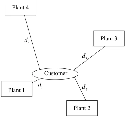
, positioned at different locations. We assume that

plants are identical (there is a dedicated production line in each plant for the customer area), and every plant can process all jobs. It takes p units of processing time to produce job j , _j j∈ , on any of the plants. Job j is denoted as N J . Each job needs to be processed on only j one of the plants without interruption. Preemption is not allowed. Each finished job should be transported from the plant on which it is produced to the customer. A job cannot be transported unless it has completed its processing in the plant. The distance of plant i ,

i∈M , to the customer is denoted as d and given in time units. Hence, in other words, it _i

takes the transporter d units of time to go from plant i to the customer. It is assumed that i the travel time from a plant to the customer is equal to the travel time from the customer to that plant. Distribution of finished jobs from the plants to the customer is done by a single

(41)

truck which can carry up to K jobs. Loading and unloading times are assumed to be negligible. Only direct shipments are allowed. To the best of our knowledge, in practice, companies with multiple plants try to allocate those plants so that they will be able to serve as many warehouses as possible. Since they do not require the plants to be in close proximity of each other, it can be assumed that those plants may be distant to each other. Therefore, our assumption of direct shipments is reasonable. Initially, the truck is assumed to be located at the customer area and for convenience each shipment (i.e. each visit of the truck to a plant) will be called a trip. A simple representation of plant locations and their distances to the customer area can be seen in Figure 3.1 for an example with 4 plants.

Figure 3.1: A representation of plant locations and distances to the customer area

Without loss of generality, throughout this thesis, the plants are named according to their distances to the customer area. The plant with the smallest distance is called Plant 1, the one with second smallest distance is called Plant 2, and so on. Again without loss of

2

d

Customer

Plant 4

Plant 1

Plant 3

1

d

Plant 2

3

d

4

d

(42)

processing time is referred to as job 1, the one with second smallest processing time is called job 2, and so on. Hence, d₁≤d₂ ≤....≤d_m and p₁≤ p₂ ≤....≤ p_n.

For job j , produced on plant i , to be transported from that plant to the customer at

time t , there are two conditions to be satisfied:

• Job j needs to have completed its processing on or before time t ,

• The truck should arrive at plant i on or before time t and should still be there at time t .

As common in the relevant literature on integrated scheduling of production and distribution operations, the completion time of job j is determined as the time that job reaches the customer. In our study, the objective is to minimize the total completion time of all jobs. A solution constitutes the following:

o Assignment of the jobs to the plants

o Scheduling of production of jobs at each plant o The route and schedule of the truck

o Assignment of the jobs to the trips

Suppose that jobs are assigned to a plant set M ′ , M′ ⊆M . The route of the truck is

the order truck visits the plants in M ′ . For example, if the truck visits first Plant 2, then Plant 1, and then Plant 2 again, the route of the truck is Plant 2 – Plant 1 – Plant 2. Determining the schedule of the truck means determining the time truck leaves each plant on its route.

In this study, we consider a single planning horizon and we aim to send the jobs to the customer as soon as possible within this planning horizon. Viewing the customer area as a warehouse, the length of this planning horizon depends on the demand amount of the warehouse.

(43)

In Chen (2008), MP notation is used for multiple decentralized plants. Denoting the completion time of job j N∈ as C , and using the three-field notation as in Lee and Chen _j

(2001), our problem can be denoted as MP→1v=1,K ≥1

∑

Cj . Here MP→1 means from multiple plants to a single customer area, and v=1,K ≥ means using a single truck 1 with a capacity of K . The following theorem holds for our problem.

Theorem 1. There exists an optimal schedule that satisfies the following conditions for each plant:

(i) If J is processed earlier than_i J , then _k J leaves the plant no later than_i J . _k

(ii) Jobs are processed in non-decreasing order of processing times in each plant. (iii) There exists no idle time between job processing in any given plant.

(iv) The transporter either leaves the plant immediately as it arrives or at the

completion time of a job.

Proof:

(i) Suppose that there exists an optimal schedule in which J is processed earlier _i

thanJ but leaves the plant after_k J . While having the same transportation schedule, if we _k

interchange the processing positions of these jobs at the plant such thatJ is processed earlier k

thanJ , the total completion time will not change. If we apply the same interchange _i

procedure to all necessary job pairs, we will have a transportation sequence which is the same with the processing sequence.

(ii) Consider an optimal schedule where jobs are not processed in non-decreasing order of processing times (SPT order). Then there exists at least two adjacent jobs J and i J k where J is processed before _i J and_k p_i > p_k. If J and _i J are transported on the same trip, _k

then interchanging the processing positions of these jobs at the plant will not increase total completion time. However, if J and _i J are not transported on the same trip, interchanging _k

(44)

the positions of these jobs may decrease the total completion time by decreasing the start times of the trips on which these jobs are transported.

(iii) If there exists idle time between job processing, we can move the jobs succeeding the idle period earlier without increasing the total completion time.

(iv) Suppose the vehicle leaves the plant neither as soon as it arrives there nor at the completion time of processing of a job. Then we can move subsequent trips earlier to either the arrival time of the truck at the plant or to the process completion time of the most recently loaded job and in this way decrease the total completion time.■

The following section aims to more precisely convey the parameters given in a problem instance as well as the structure of a desirable solution by considering a numerical instance.

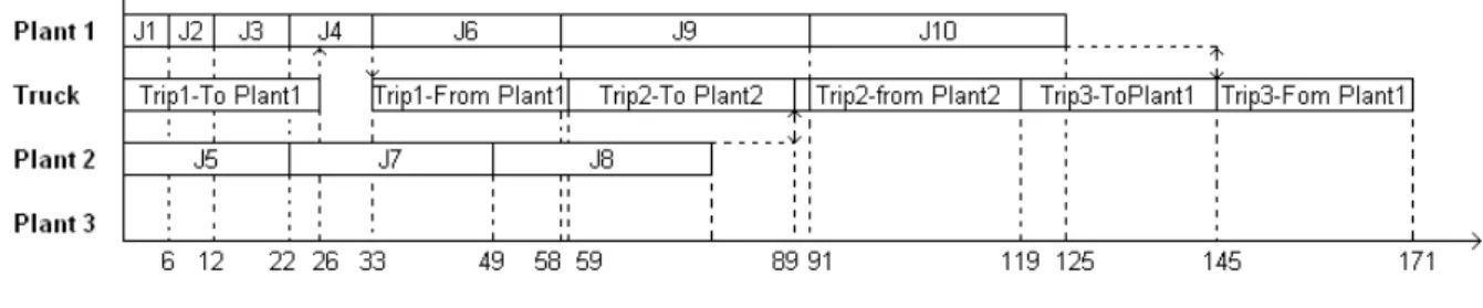
3.1. Sample Problem

Suppose that we have 10 jobs to be processed at a subset of 3 plants, and to be transported with a truck that carries at most 4 jobs in a trip. First, the plants are sorted in non-increasing order of their distances to the customer and reindexed, and the same procedure is applied for the jobs with respect to their processing times. After sorting, the distances of the plants can be listed as d =

{

d d d₁, ,₂ ₃

} {

= 26,30,37

}

whereas the processing times of the jobs

can be listed as p=

{

p p p p p p p p p p₁, ₂, ,₃ ₄, ₅, ₆, ₇, ,₈ ₉, ₁₀

}

=

{

6,6,10,11, 22, 25, 27, 29,33,34

}

.

As can be seen in Figure 3.2, the optimal solution to this problem assigns jobs

{

J J J J J J J1, , , , , ,2 3 4 6 9 10

}

to Plant 1, and the rest to Plant 2. As have been stated in Theorem

Integrated scheduling of production and logistics operations of a multi-plant manifacturer serving a single customer area