A microscopic approach to phononic energy transfer in nano structures

■& E M £ T D ш т ж ѣ ё : ^ с

im

sTHucTUHEs

“О THE D£EAHT^Л.£■^Π“‘ Di'^ 'r^r¡ ··

“Î O F TT?iD ñ hi %.. A W ' í ь4 F i » ^ ·» -Él ^ ;т w ^ py ^ íVTí V ,. D. yiAM,· ,.>V. l^íl*».; >»^«*í ; j · - г ч г R E O U IF ïE i'^ S .--T S α 'vi' "·'*/' '►·ΐΛ*·ν· ’l» Λ ■*«·*#< ^ í W ^ M .«^í· ^ r , ^ c ,,-"Гc-4/Тo:¡rСу ^ £ ·:\τ

A MICROSCOPIC APPROACH TO PHONONIC

ENERGY TRANSFER IN NANO STRUCTURES

A THESIS

SUBMITTED TO THE DEPARTMENT OF PHYSICS AND THE INSTITUTE OF ENGINEERING AND SCIENCES

OF BILKENT UNIVERSITY

IN PARTIAL FULFILLMENT OF THE REQUIREMENTS FOR THE DEGREE OF

MASTER OF SCIENCE

By

Altiig Ozpineci

September, 1999

о

32

_■05Я

(

IS

S

I certify that I have read this thesis and that in my opinion it is fully adequate, in scope and in quality, as a thesis for the degree of Master of Science.

;

Prof. Dr. Salim Çıracı(Pri;icipal Advisor)

I certify that I have read this thesis and that in my opinion it is fully adequate, in scope and in quality, as a thesis for the degree of Master of Science.

" Prof. Dr. Cemai~¥arabik

I certify that I have read this thesis and that in my opinion it is fully adequate, in scope and in quality, as a thesis for the degree of Master of Science.

s - . · ■ • s .

Prof. Dr. Şinasi Ellialtioğlu

Approved for the Institute of Engineering and Sciences:

Prof. Dr. Mehmet JE^ray

Director of Institute of Enginagring and Sciences

ABSTRACT

A MICROSCOPIC APPROACH TO PHONONIC

ENERGY TRANSFER IN NANO STRUCTURES

Altug Ozpineci

M.S. in Physics

Advisor: Prof. Dr. Salim Qiraci

September, 1999

Understanding of mechanisms for the energy transfer from and/or through nano particles in contact with the large samples have become important in various biological processes, molecular electronics and friction. In this thesis, the phononic heat conductance of an atomic wire between two reservoirs, and the vibrational relaxation of an atom adsorbed on a surface is studied. The former problem is studied using the Keldysh formalism which yields the steady state properties of the system. The dependence of the total conductance on temperature, on the number of atoms in the wire and on the coefficient is studied. It is found that the conductance shows quantal structure similar to the electronic counterpart.

The reduced density matrix is used to study the latter problem. The time evolution of the reduced density matrix has been evaluated for an arbitrary system coupled to a heat bath. The formalism is then applied to study the vibrational relaxation of an atom adsorbed on a surface. The frequency depen­ dence of the relaxation time is also determined.

Keywords and Phrases: Heat Conductance, Keldysh Formalism, Phononic

Heat Conductance Quantization, Reduced Density Matrix, Vibrational Relax­ ation

ÖZET

NANO YAPILARDA FONONLARLA ENERJİ

TAŞINIMINA MİKROSKOPİK BİR YAKLAŞIM

Altuğ Ozpineci

Fizik Bölümü Yüksek Lisans

Danışman: Prof. Dr. Salim Çıracı

Eylül, 1999

Daha büyük cisimlere bağlı nano cisimlerden ve/veya bunların üzerinden enerji akışının mekanizmalarini anlamak, pek çok biyolojik , moleküler elektronik ve sürtünme ile ilgili olayı anlamak için önemlidir. Bu tezde, iki rezervuara bağlı tek boyutlu atomik bir telin fonon kaynaklı ısı iletkenliği ile bir yüzey üzerine yapışmış bir atomun salınımının sönümü incelendi, ilk problem, incelenen sis­ temin durağan durumu hakkında bize bilgi veren Keldysh formülasyonu kul­ lanılarak incelendi. Telin toplam ısı iletkenliğinin sıcaklığa, atom sayısına ve

katsayısına bağlılığı hesaplandı. Isı iletkenliğinin de, elektrik iletkenliği gibi kuvantal bir karakter gösterdiği bulundu.

ikinci problemi incelemede indirgenmiş yoğunluk matrisi kullanıldı. Isı rezervuarına bağlı herhangi bir sistemin indirgenmiş yoğunluk matrisinin za­ man içinde nasıl geliştiği hesaplandı ve bir yüzey üzerine yapışmış bir atomun salınımının sönümü incelendi. Durulma zamanının frekansa bağımlılığı belir­ lendi.

Anahtar Kelimeler ve ifadeler: Isı iletkenliği, Keldysh Formülasyonu, Isı

iletkenliği Kuvantizasyonu, indirgenmiş Yoğunluk Matrisi, Salınırnsal Sönüm

ACKNOWLEDGMENTS

I would like to express my sincere gratitude to Prof. Dr. Salim Çıracı for his supervision. His patience and expert guidance brought my research up to this point.

I am greatful to my family for all the self-sacrifices they have made in order to grow me up to this point.

I owe thanks to all my friends especially Mithat Unsal, and Özgür Çakır for all they have done for me.

The most thanks goes to Özlem Sert, who has helped me out of all the obstacles of life since my undergraduate years.

C o n te n ts

1 Introduction 1

1.1 Density M a t r i x ... 3

1.2 Definition and Some of the Properties of the Density Matrix . . 4

1.3 Systems Interacting with the Environment and the Reduced Density M a t r i x ... 5

2 K eldysh Formalism Approach to Heat Conduction Through A tom ic W ires 7 2.1 Keldysh F o rm alism ... 8

2.2 M o d e l ... 10

2.2.1 Current O p e ra to r... 12

2.2.2 Analytical C alculations... 13

2.3 Numerical Analysis and D iscu ssio n ... 14

3 R educed D ensity M atrix Approach to V ibrational R elax­ ations 23 3.1 Evolution of the Reduced Density M a trix ... 24

3.2 The Model Hamiltonian 26 3.3 Numerical Analysis and D iscu ssio n ... 27

4 Conclusion 35

A Eq. 2.1 37

B Eq. 2.23 40

C Eq. 2.27

C.0.1 Free Greens Functions of the Wire

C.0.2 Free Greens Functions of the Reservoirs

42

44

45

List of Figures

2.1 A schematic description of the model used in the present study. The balls represent the atoms with mass m ... 11

2.2 The graphs of k{w) at various temperatures for (a)

N=1; (b) N=5; (c) N = 1 0 ... 19

2.3 The graph of the dependence of the total conductance, k, on O = at various temperatures, (a) N=1; (b) N=5; (c) N=10 21 2.4 The graph of the dependence of the total conductance, k, on

temperature at = ^ for = 5 ... 22

2.5 The dependence of the total conductance on the number of atoms at various temperatures and for = wo, and

= V T = T 22

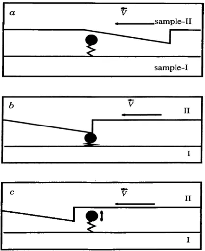
3.1 An adsorbed atom between the surfaces of two samples, one of which move with a velocity v. (a) There is no interaction be­ tween the sample-II and the rest of the system, (b) the adatom is squeezed, absorbing some of the translational energy of sample- II. (c) the adatom is suddenly released causing it to oscillate and the interaction between the sample-ll and the rest of the system is again neglected... 28

3.2 Calculated decay profiles, for the energy of the vibrating atom for various O’s... 33

3.3 Dependence of the relaxation time, r, on the vibrational fre­ quency, Q, of the adsorbate... 34

A.l The time loop along which the operator 7c orders its arguments. 38

C h a p ter 1

In tr o d u c tio n

Understanding the energy flow through and from substances is essential for a fundamental understanding of various processes in nature ranging from the reactions in the living organisms to various applications in device physics. In itself, controlling the rate of energy flow, being able to increase or decrease it, has a great importance for various applications.

In microelectronics, the quality of growth of silicon wafers and SiGe, Al- GaAs heterostructures is essential for the operation of the devices. Nowadays, significant resources have been allocated to understand the growth mechanisms so that conditions can be established to grow defect-free crystals and wafers. The growth process involves several complex and stochastic phenomenon tak­ ing place in the atomic scale. An important and fundamental issue one has to clarify is how the huge energy emerged from the formation of chemical bonds between incoming atoms and surface atoms. The dissipation of this energy is essential for the quality of the surface, where the electronic device will be pro­ duced. Clearly the question one has to address here is how the energy released from the bond formation dissipates through the sample, what is the time scale for the dissipation? Another important issue is how the energy generated in an electronic device can dissipate as the size of an electronic device becomes smaller and smaller. In fact, this problem seems to be a factor that limits the miniaturization of devices.

In solar collectors [1], it is important that the collected energy should be transferred into the bulk before it is reemitted to the surrounding. In order to make more efficient solar collectors, the rate of energy transport into the bulk

should be increased. In the case of friction, where two surfaces rub against each other, heat is generated. The rate of heat transfer is important for the dissipation of the mechanical energy and for the wear of surfaces.

In living organisms, most catalytic activity takes place on surfaces [2], hence the reactions can be considered as a set of transitions between various energy levels whose understanding requires a deep understanding for the processes at the surfaces, especially the processes involving energy transfer.

In recent years, there have been extensive theoretical studies on phonon transport and energy relaxations using various methods, including the Kubo formula for heat conductance [3, 4, 5, 6], Landauer type phenomenological energy flux [7, 8, 9, 10], Golden Rule [11, 12], and Langevin type equations [13, 14, 15, 16]. On the experimental side, vibrational relaxations have been studied extensively [17, 18, 19, 20, 21], but to the author’s knowledge, there is no experimental study on the conduction of ID wires (for a review of the present situation see e.g. [22]). The Kubo formula yields just the first order response of the system to an external disturbance, and expresses the conductivity tensor in terms of the current-current correlation functions in equilibrium [6]:

i + (1-1)

c — ►0+ , u>—+-0k qI V Jo J—oo

where ks is the Boltzman constant, V is the volume of the system, represents the /¿‘^-component of the heat current, and (...) denotes the thermal averaging in equilibrium. In cases where the considered system cannot be described by linear response theory, it is not applicable. But in situations where it is applicable, it gives a microscopic description of the phenomenon.

A Landauer-type phenomenological energy flux is given by (for the deriva­ tion see [24]):

•^ = E j ( “ ( n .K i* ) ] - »2K (4)D C~(*) (1.2) where ni(2) are the phonon distributions at the left(right) reservoirs, and C,n{k) is the transmission probability for the phonon. Eq. 1.2 gives a macroscopic description for the heat transport. In most cases, the transmission probabil- itVi (n{k), is assumed to be unity or that it is given by matching continuum solutions for the elastic waves at the boundaries. For nanosystems, where the discrete atomic nature of the structure becomes pronounced, the use of con­ tinuum theory to determine the transmission coefficients cannot be justified.

Under these circumstances, one has to develop a microscopic theory as done in this thesis to calculate the transmission coefficients and conductance. At the end of this thesis, we will present a microscopic definition for Cn{k).

The Langevin type equation describes the time evolution of the reduced density matrix of the system. They give a microscopic description of the system under study. The density matrix theory will be reviewed in the next section. A broader discussion on the density matrix theory and its applications can be found in eg. [23].

This thesis deals with the microscopic aspects of phononic energy transfer in nanostructures. Two case are considered are (î) the phononic energy transfer

and the related thermal conductance through an atomic chain coupled to two reservoirs; and (ii) the dissipation of excess vibrational energy from an adsorbed atom to the substrate. In both cases the models used to simulate the real systems have been simplified in order to reveal the essential features of heat transfer, but the approaches and formalism developed can easily be extended to more complex systems. On the other hand, in both cases treated in the thesis the approaches developed are unique and hence are expected to contribute to a better understanding of the related physical problems.

For the first case, the Keldysh’s approach for non-equilibrium but steady state is used and the energy current through a finite and uniform atomic chain mediated by phonons is calculated. The variations of thermal conductance as a function of chain parameters, and temperature are investigated. A quantum structure of thermal conductance is revealed. For the second case that has a wide range of applicability, in particular it is relevant for the energy dis­ sipation from an adsorbed atom coupled to a substrate through anharmonic interactions, the reduced density matrix approach is used. It is found that the time of equilibration is rather small and most of the excess energy dissipates within 10“ ^^ sec. The details of the work is given in Chapters 2 and 3, and conclusions are summerized in Chapter 4.

1.1

Density Matrix

For systems that can be described by a wave function, the wave function gives a complete description. Such systems are said to be in a pure state. Once the

wave function is known, everything about the system, within the limitations of Quantum Mechanics, is known. But for most systems, including systems cou­ pled to the environment, description by a single wave function is not possible, it is not in a pure state. Such systems are said to be in a mixed state. In such cases, the system should be described by the density matrix.

1.2

Definition and Some of the Properties of

the Density Matrix

For most system, one can at most know the probabilities, p,, that the system is in a state described by the wave function |V’i)· In such cases, in order to calculate the expectation value of an operator, one should take the statistical average besides the quantum average, ie.:

(o) = E p . ( * W i ) .

i

If Eq. 1.3 is rearranged as:

(O) = Y,'^Pi{tl>i\0\n){n\ii}

(1.3)

n I

\ C*|n)

T r f x ; p i | V ’.:)(V'i|l O , (1.4)

where {|n)} is an orthonormal basis for the Hilbert space of wave functions, the definition of the density matrix easily follows as:

i

and the expectation value of any operator can be written as:

{0) = TrpO .

Note that the wave functions |V>,) need not be orthogonal.

(1.5)

(1.6)

Several properties of the density matrix follows immediately from its defi­ nition, Eq. 1.5.

• Trp = J2iPi = 1·

• Trp^ = J2iP^ ^ 1, 3,nd the equality sign holds if and only if it is in a pure state.

• The density matrix is hermitian, i.e. p^ = p. Therefore it is always possi­ ble to find a suitable basis in which the density matrix can be represented by a diagonal matrix, the diagonal entries being the classical probabil­ ities. If the system is in a pure state, in its diagonal form, all but one of the diagonal elements will be zero, and the non-zero diagonal element will be 1.

These properties are independent of the representation used for the density matrix. Eq. 1.5 is just one of the representation in which it is easy to show these properties.

Since the density matrix is written in terms of the wave functions, its time evolution is also determined by the time evolution of the wave functions, hence, contrary to other operators in Quantum Mechanics, it is time dependent in Schroedinger picture, and time independent in Heisenberg picture. Its time dependence can be written as:

P(i) = J2Pi\Mi))iMl^)\

I

=

(1.7)

1.3

Systems Interacting with the Environ­

ment and the Reduced Density Matrix

In general, one does not deal with an isolated system and it is mostly not necessary to consider all of the interacting parts, which would require one to consider all the universe. In such a case, the density matrix of the whole system contains unnecessary information.

Let p be the density matrix of the whole system A + B where the A and

B subsytems interact with each other (in fact even if they had interacted for a

short time in the past, they have to be described by densitymatrices). Let Oa

be the operator corresponding to an observable about the A system. Then its expectation value is given by:

{Oa) = TtOaP. (1.8)

The Tr appearing in Eq. 1.8 can be written in two parts: trace over the degrees of freedom of the /l-system, T r^, and trace over the degrees of freedom of the 5-system, Ttb- Since, by assumption, Oa does not affect the degrees of

freedom of the 5-system, it can be taken out of Trs] ie.

TrA Tv bOaP

71771 (1.9)

Y^^{n\OA |n)^

Th \ 771 / (1.10)

Tt aCa (Tt b p) (1.11) The quantity in parenthesis contains all the information about the A-system and is called the Reduced Density Matrix. It will be denoted by pR. It has the same properties listed in the preceding section. Its time dependence is determined by the time dependence of the density matrix of the whole system by

C h ap ter 2

K eld y sh F orm alism A p p roach

to H ea t C o n d u ctio n T h rou gh

A to m ic W ires

In studying non-equilibrium systems, in some cases it is more suitable to deal with a time independent density matrix, in which case one can use the Heisen­ berg picture, or it can be more suitable to use the time dependent density ma­ trix, i.e. in the Schroedinger picture. In this chapter, heat conduction through an atomic wire between two reservoirs will be studied in the Heisenberg pic­ ture, or more precisely the Interaction picture. The formalism employed is the Keldysh formalism.

In equilibrium field theory, the interaction is adiabatically turned on at

t = —oo and it is adiabatically turned off at i = -foo, and it is assumed

that the state obtained after this switching on and off of the interaction is the initial state upto a possible phase. This assumption can be justified only in the case of equilibrium and if the considered state in non-degenerate, but breaks down otherwise. In transport, for example, when the interaction is turned on, particles are transferred and they do not come back when the interaction is adiabatically turned off. In the Keldysh formalism, this assumption is not done, the state is first evolved from t = —oo to f = -|-oo and then back to

t = —oo again so that one does obtain the initial state. Keldysh formalism

has been applied to the study of electron transport (see eg. [25, 26, 27]), but to the authors’ knowledge, it had not been applied to the problem of phonon

The organisation of this chapter is as follows: in Sec. 2.1, a review of the Keldysh formalism will be presented (see eg. [28]). In Sec. 2.2, an analytical treatment of the heat current through the uniform atomic wire will be carried out and the results will be studied in detail in Sec. 2.3. As much as possible, the details of the calculations will not be presented in the main body of the text but will be given separately at the Appendices at the end of the chapter.

transport.

2.1

Keldysh Formalism

The Keldysh formalism gives a means of calculating the properties of systems that are not in equilibrium but are in steady state. In steady state, the expec­ tation value of any operator,(9, can be expressed as:

(O ) = Tr (pO) Trip)

Tr (p o ^ O (0+)e-^

(2.1)

where {O)o = TrpoO. In Eq. 2.1, it is assumed that the system has the density matrix po and the Hamiltonian TL^ dX t = —oo. Then, the interaction, described by the Hamiltonian TLinti is turned on and the density matrix of the system evolves to the steady state density matrix, p. The time loop, C, is defined to be the path that goes from t = —oo to t = +oo and then from

t = -|-cx) back to i = —oo. The times which are on the upper branch that goes

from t = —oo to Z = +00 are labeled by a (''■) and the times which are on the lower branch that goes from t = -j-oo back to t = —oo are labeled by a (“ ). The operator Tc which appears in Eq. 2.1 is the path ordering operator which orders the operators according to their positions on the time loop. If all the times have the label (■*■), the Tc reduces to the time ordering operator and if all the times have the label (“ ), then it reduces to anti-time ordering operator. Expanding the exponential in Eq. 2.1, yields a perturbation expansion for the average of the operator. By the use of Wick’s theorem, the expansion can be given a diagrammatic interpretation. In terms of the diagrammatic expansion,

Eq. 2.1, can be simplified to;

connected

(

.

)

where the subscript connected indicates that only the connected diagrams should be considered.

Let us define the two point correlation functions of the displacement of the atoms of the wire as:

where X{ is the displacement of the wire atom and Q = + , — ·

If one defines the matrices

a . ( t - t ' ) = ( ' ' ' s r r ( i - n s a - 1' ) = ( (2.3) (2.4) (2.5)

where the E ’s are the self energies, the Dyson equations can be written in a compact form as:

Gij{t ~ = ^Oij{t — t') +

+ Y , f - n ^ k ' A t ' " - i') (2.6) j'k'

where ^Gij{t — t') is the unperturbed Greens function. In terms of the Fourier transformed Greens function, Eq. 2.6 can be written as:

Q i j { w ) = ° G i j ( w ) + Y ° Q i j ' { w ) ' S j ' k ' { w ) Q k ' j { w ) . j' k'

Diagrammatically, the Dyson equations can be represented by:

(2.7)

<

>

I I

I

where the thin lines represent the free propagators and the solid lines represent the full propagators.

Note that not all the Greens functions and the self energies are independent. They satisfy:

^ + + _ ^ + - _ ^ - + =

E++ + E— + E+- + E -+ = 0

Using these relations, the matrices Qij and E,, can be transformed to:

(

.

)

O'*

sg

=

(

.

)

where CTy is the second Pauli matrix:

(Ty — 0

- i

1

After this transformations, the Dyson equations, Eq. 2.6, become:

S U M = ° e . » - E ”e 5 (''')s .v (» )e i? ,(" ') (2.12 )

i'j'

= V i ( » ) - E “5;;.(t»)si,,(«,)0'),(·») (2.13) s 5 '(» ) = ° e S '( > » ) - E ° 5 .i’(»)s?i(>»)ej),(<»)

i'j'

- E ° S .? (u.)E?,,(u,)0« (t„) - j : ”0i,(»)E i,,(»)S 'i).(«.)(2.14)

2.2

Model

Suppose th at we have two reservoirs with temperatures Th and T/j and are described by the Hamiltonians T-ii, and Tin respectively. Consider a ID, uni­ form atomic wire of N atoms connecting the two reservoirs described by the Hamiltonian:

N „2 N I

w^ = E ¿ + E І( -.- -.+ .)^

z = l ¿=0 ^

(2.1.5)

with fixed boundary conditions xq = xyv-M = 0· The system is shown in the

figure below.

Figure 2.1: A schematic description of the model used in the present study. The balls represent the atoms with mass m.

In this Hamiltonian, we assume N identical masses all of which are connected to its nearest neighbours and the ones at the ends connected to the surfaces, which are assumed to be rigid, by identical springs. This model is over simplified to represent a real physical system quantitatively but we believe that it will grasp the qualitative features of heat conduction through atomic wires. The interaction between the wire and the reservoirs can be described, at the lowest order, by the Hamiltonian:

'Hint = AlUlXi

+

,

where u's are the lateral displacements of the reservoir atoms which interact with the wire. In this interaction term, it is assumed that only one atom from each reservoir is interacting with the wire and only the longitudinal modes are considered, generalizations to include other interactions and other modes is possible. Due to this interaction, the states of the wire are broadened. If the interactions of the wire atoms with other reservoir atoms is also taken into account, the broadening will be more pronounced.

At i = —oo, before the interaction is turned on, the initial density matrix is given by.

(2.17)

where Z = Tre is the partition function of the whole sys­ tem at time t — —oo. Note that although at i = —oo, the initial density

m atrix depends on the initial temperature of the wire through /?5 = at steady state, no physical quantity should depend on it.

2.2.1

C urrent O perator

The operator corresponding to the current at the contacts can be obtained from the continuity equation written in the form:

(2.18) where e is the total energy operator of the wire and Jr{l) is the operator for the current leaving(entering) the wire at the junction at the B,{L) reservoir. Let e = Tisi then Eq. 2.18 is satisfied by the choices:

r Jl = ---ulPi , m Jr — — w,ßpyv · m (2.19)

(

.

)

Note that the current operators are proportional to the velocity, u,· = of the corresponding atom. One might argue that there is no a priori reason for the choice e — Tis· Our attitude was that the energy of the wire appearing in the continuity equation should be a characteristic of the wire only, hence should not contain any operators related to its environment. An alternative argument could be: the energy of the wire should be the sum of all the terms in the Hamiltonian containing the wire operators. Hence it would be he difference in the Hamiltonian if the wire was absent. But the two approaches yields the same result due to the identity:

A i t ^ ( » i ( 0 ) j : ,( l '- i ) ) = - M l- ^ {ul{0)x i{1' - t ) )

= -ML-^{uL{t)xi{t'))

Ml

m

(tl £,(()?,(i')),

2

21

where Ml and pL are the mass and momentum, respectively, of the left reservoir

atom which interacts with the wire. In the derivation, we have used the time

translational symmetry of the steady state. A similar derivation can be used to show:

m (2.22)

where Mr and pR are the mass and momentum, respectively, of the right reservoir atom which interacts with the wire. In this work we will concentrate

on J = {Jr) and by energy conservation {Jr) = {Jr)·

2 .2 .2

A n a ly tic a l C alcu lation s

Using the Wick theorem, the current, J can be expressed as (details can be found in Appendix B)

J= - E f

a=l,N·^

where the a summation, in fact, represents a summation over all the contacts. In our case there are just two contacts but generalization to the other case is possible. With the interaction described by Eq. 2.16, the self energy can be calculated exactly:

^ i j { w ) = E i i { w ) 6 { i 6 j i + TiRN{w)6iN6jRj

where ^u{w) are the Fourier transforms of

E“ (i - (') = (-!)<■<■

,

(2.24)

(2.25)

(2.26) Here (— = 1 if Cl = C2 and (—1)^’^^ = —1 if Ci C2 Substituting the S into Eq. 2.7, one can solve for the exact Greens function, Q. Once they are substituted into the expression for the current, the result can be simplified to

J = 27T dwg’^{w)g^{iv) x

hiu det QiNi^)-

-{n'^{w) - n^{w))

2Mrw 2Mrw

where det^i/v(to) = determinant of the 2 x 2 Greens function matrix and ng^^\u) = (e^M«)'*‘^ — 1)“ ^ are the Bose distribution func­ tions at the left(right) reservoirs. The details of the derivation can be found in the Appendix C. The determinant can be decomposed as,

det Qin = det + det (2.28)

where det describes the contribution of balististic phonon transport and det describes the phonon tunneling contribution. Hence the total current can also be decomposed as the sum of the tunneling current and ballistic cur­ rent.

Note the similarity between this result, Eq. 2.27, and the Landauer type expression, Eq. 1.2 which, after a change of variables, can be written as :

J = dwhw{rig{w) - nQ{w))Tm{w) (2.29)

where Tm{w) is the transmission coefficient for a phonon of frequency w at the branch to be transmitted from the left reservoir to the right reservoir. In our case, if we allow the reservoirs to have various phonon branches, the total density of states appearing in Eq. 2.27 should be replaced by sums over the density of states of each branch, in which case, we obtain for the transmission coefficient for a phonon of frequency w at the branch of the left reservoir to the branch of the right reservoir to be:

= (2^? ( ^ )

Eq. 2.30 is important because, to the authors’ knowledge, it is the first non- phenomenological microscopic derivation of the transmission coefficient, and contrary to other expressions used in the literature, it takes into account the discrete nature of the system.

2.3

Numerical Analysis and Discussion

In all the calculations, both reservoirs are assumed to be identical Debye solids except their respective temperatures. Let

J{Tl, Tb) — i dxJ{xLoo,TL,Tfi)

Jo (2.32)

J{uj, T) can be considered as the heat current density at the frequency u. Then

the heat conductance density at the temperature T can be defined as: J ( r o ,r + A T ,r )

Kiw/r) = lim

'' > A T-*0 _AT (2.33)

so that the total conductance is given by,

K> = [ dxK{xw[)^ T ) . (2.34)

For the numerical data, we used hu>^ - huj^ = Ulod — 37.6 meV,

Ml = Mr = 56 amu, m = 28 amu, and Al = Ar - -1 9 J/m ^. The phonon

density of states is represented by the 3D Debye density of states,

/(^)(-) =

- - )

Wd

(2.35)

where wp is the Debye frequency and 0 is the step function. It should be noted that the contribution of the surface phonons are not taken into account.

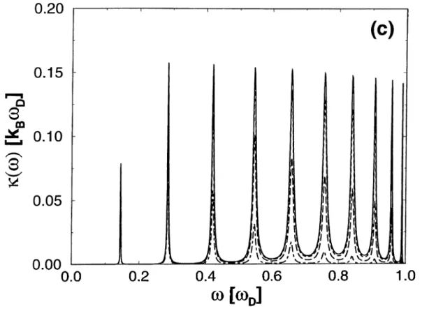
In Figs. 2.2a, 2.2b and 2.2c, the dependence of the conductance density on the frequency, u, is shown at various temperatures and for = 1, = 5, and A^ = 10 respectively. The resonances at the eigenfrequencies of the wire and their broadening are clear. The heights of the peaks are almost independent of the number of atoms in the chain, while they become narrower as N becomes larger. This can be understood in terms of the weakening of the coupling constant of each mode to the reservoir modes which is proportional to .

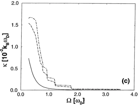
In Figs. 2.3a, 2.3b and 2.3c, the dependence of the total conductance on the coefficient is shown. Contrary to the electronic counterpart, the steps are clear at high temperatures whereas they are lost at lower temper­ atures. As increases, the eigenfrequencies of the wire increase, and as one eigenfrequency crosses the Debye frequency, it no longer contributes to the conductance, and hence there is a fast decrease at the total conductance. The more separate the eigenfrequencies are, the longer the plateaus. At high temperatures, all of the eigenmodes contribute to the conductance, hence there are several steps. But as can be seen in Figs. 2.2, at low temperatures, there is very few high frequency phonons at the reservoirs, hence the modes corre­ sponding to the higher eigenfrequencies do not contribute; the corresponding “channel” is closed at lower temperatures. Following comments related with Fig. 2.3 are in order: (i) The step behavior of electrical conductance is ob­ tained by changing the width of the constriction or by stretching the metallic wire between two electrodes. In the present case, the step behavior of k can be

realized to some extent by varying k and m, and also top. Of course top is an artificial cut-off due to the Debye model. In a real crystal, the cut-off of o;(k) at the zone boundary has to be taken into account. Cut-off frequencies can

be modified by applying strong external pressure so that the lattice spacing is modified, and the eigenfrequencies of the wire can be modified by stretching the wire. According to the present result, if the atoms of the chain are replaced by their isotopes, the value of k changes even if all other parameters are kept

the same, (n) In the case of quantum ballistic conductance of electrons, the step heights (or jumps in the electrical conductance, a, are normally integer multiples of 2e^/h depending on the degeneracy of the channel. The phononic thermal conductance step heights are inversely proportional to N. {in) The step structure shown in Fig. 2.3 can be modified if there is surface phonons at the gap. It can be argued that the present model and the measurement of conductance can be used to investigate the surface phonons, {iv) In calculating the step structure, the broadening of the modes of the atom is fully taken into account, within our model, which smeared the step. This smearing is more pronounced for the first several steps, since the higher eigenmodes are more closely spaced, and hence they overlap due to the broadening. If interaction with more then one reservoir atom is taken into account, as discussed in the text, the extra broadening would further smear out the steps. Therefore it is possible the this extra broadening, which is present in realistic systems, might cause the steps to disappear completely.(u) The anharmonic coupling which is not taken into account here, may modify the step behavior especially for very large and for u>i > u>d

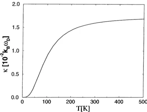
In Fig. 2.4, the dependence of the total conductance on temperature is shown. In this plot it is assumed that and since at this frequency, the conductance is almost independent of the number of atoms, it is only shown for N = 5.

In Fig. 2.5, the variation of the total conductance at various temperatures as the number of atoms is increased is shown. As is seen from the figures, for the total conductance is almost independent of the number of atoms. The total conductance for a single atomic wire is less then the total conductance for NQ^2. The difference is due to the tail of conductance density which extends beyond the Debye frequency as can be seen in Fig. 2.2a. For y ^ = u>d,

there are fluctuations in the total conductance. This fluctuations are due to the fact that in the first case all the modes contribute to the conductance since the Debye frequency is greater than all the eigenfrequencies of the wire, whereas in the second case, the Debye frequency lies within the spectrum of the wire. Hence the ratio of the contributing modes to the total number of modes

fluctuates, but the fluctuations diminishes as the number of modes increases.

Finally, it may be interesting to find out how the total thermal conductance of the the atomic wire with N > 2 and ^ \s compared with the

universal value of conductance [7, 8, 9] kq — which is proportional to the tem perature T. In out case, if one Taylor expands the conductance expression, Eq. 2.34, in terms of the temperature, the first non-zero term is proportional to contrary to the results in [7, 8, 9].

8ΐ

04

8Ό

9Ό

VO

го

Ο Ό

О О

О

90

Ό

Ä

S

91-Ό

ого

04

80

90

PO

го

Ο Ό

О О

О

90

Ό

ѳ;

s

91-Ό

ого

0.0

0.2

0.4

0.6

0)[coJ

0.8

1.0

Figure 2.2: The graphs of «(w) at various temperatures for (a) N=1; (b) N=5; (c) N=10

0.0

0.5

1.0

1.5

2.0

2.5

Q [ c o J

Figure 2.3: The graph of the dependence of the total conductance, /c, on ii at various temperatures, (a) N=1; (b) N=5; (c) N=10

0 100 200 300 400 500

T[K]

Figure 2.4: The graph of the dependence of the total conductance, k, on tem­

perature at ^ for iV = 5

Figure 2.5: The dependence of the total conductance on the number of atoms at various temperatures and for = y /^ = u;/), and 0 = y ^ —

C h a p ter 3

R e d u c e d D en sity M a trix

A p p ro a ch to V ib ra tio n a l

R elcixation s

In this chapter, a Redfield Theory-like approach is developed(for the derivation of the Redfield theory and some of its applications see eg. [33, 34, 23]) for calcu­ lating the time evolution of the reduced density matrix in the Schrôdinger pic­ ture. The result is then applied to study the relaxation of the non-equilibrium phonon distribution taking into account the non-equilibrium properties of the system and then the method is applied to study the vibrational damping of an adsorbed molecule on a surface.

Considering an atom adsorbed on the surface of a sample, with vibration frequency i), in general there are two possible decay modes, i) it can create electronic excitations in the metal, eg. create electron-hole pairs, or ii) it can create phononic excitations. In this article our interest will be on the phononic dissipation. If ii ~ n Wo where tvo is the maximum phonon frequency of the sample(for a Debye solid it is the Debye frequency wo), the excitations can decay only by the creation of n phonons in the sample [19]. hbr large

n, this contribution is in general negligible. For systems such as the Cu-CO

stretch vibration, Î2 ~ 1.5 lUo and decay by creating two phonons might be an important mechanism for the vibrational damping of the molecule.

In [12] two and three phonon contribution to the dissipation of the Cu-CO

stretch vibrations is studied using Golden Rule formula. In this work we will study the same system using the Redfield theory-like approach for various Q’s to understand the dependence of the dissipation rate on the coupling between the sample and the adsorbed atom. The organization of the paper is as follows: In Sec. 3.1, we calculate the time evolution of the reduced density matrix which allows one to take into account all non-equilibrium properties of a system and also takes into account possible coherence and incoherence effects (for the properties of density matrices see eg [23]). Possible limitations on the obtained evolution is also discussed. In Sec. 3.2 a model system is proposed which is analyzed and solved in Sec. 3.3.

3.1

Evolution of the Reduced Density Matrix

In studying the dynamics of systems coupled to the environment, it is most natural to use the Reduced Density Matrix (RDM) formalism. The time de­ pendence of the RDM of the system can be obtained from Eq. 1.12. Let

7^ = 'his + 'hCr + 'hiint 1 (3-1) where 'Ks·, 'Hr are the system and reservoir Hamiltonians, respectively, and

Hint describes the interaction between them. We will assume, without loss of

generality, that

Hint = Y,QsFs (3.2)

s

where Qs{Fs) acts only on the system (reservoir) degrees of freedom. The time evolution of the components of the RDM is given by

Pap{i) = Pa/3(0)e~“^“'^‘ + ^ ; (3.3)

a'P'

where hu>ap = e« — and the tensor Raa'-,pp'{i) is defined as:

= E P(£i)(a>|5(i)|a'ji){*|5*(i)l/3>) - (3-4) ij

where the scattering matrix, S{t), is defined as:

S{t) =

= 1 - 7 / dt'Hint{t')

n JO

+ J ^^1 ^ dt2Hint{t\)Hint{t2) ■■■ ('^•5) 24

Here, Ho is defined to be Ho = Ht-\· Hs- Also Hint{t) = , and

\l j ) = I7 ) ® li) with,

'Ksh) = £717)

K l i ) = Ej\j). (3.6)

In the following Greek (Latin) letters will denote the system (reservoir) degrees of freedom. In deriving this result it is assumed that the bath is always in equilibrium so that the density matrix of the whole system could be factorized as:

(7jX0I<^^) = X PR'yS P{Ej) (3.7)

where the diagonal density matrix elements of the reservoir are defined as

P{E,) = (3.8)

Here Z = J2j £ ■

Until this point, the only assumption made is that the density matrix of the whole system is factorizable which resulted in a linear equation for the components of the RDM. The applicability of this approximation should be studied carefully. This assumption is valid only if there exists a Aveak coupling between the system and the reservoir so that the tensor product states |o;j) can be considered as almost the eigenstates of the whole system. If there is a strong coupling between the system and the reservoir, or if the “reservoir” is a finite one, the density matrix of the whole system in general cannot be factorized and one has to do without this simplifying approximation.

Now, the main task is to find a suitable approximation for the tensor

Raa'-,pp'{t), once it is known, the time evolution of the RDM can be calcu­

lated.

Unfortunately, the expression obtained by straightforward application of the second order expansion of the S matrix yields a result which is valid only if the time t is short enough. To overcome this difficulty we used an iterative scheme in which we calculated the initial RDM and then evolved it one step in time, and then taking the evolved RDM as the initial RDM, we evolved it one step further. At each step, the evolution was for a short enough time. Since energy is not conserved for finite times, one has to impose the energy

conservation by hand. For this reason, the matrix elements of Hint coupling states of different energies are neglected. The calculations are similar to the ones done in scattering theory with the result

\

where the prime on the summation in Eq. 3.11 indicates that the sum should be carried out over states for which hu> =

Ejk-3.2

The Model Hamiltonian

Consider an atom adsorbed on a surface. Let M be the mass of a reservoir atom and m be the mass of the adsorbed atom. Assume that the adsorbed atom is bonded to a single atom of the sample and the interaction between the sample atom and the adsorbed atom is described by the Morse potential:

U{u - v ) = E„ - 2e-”··-''·} , (3.12) where u and v are the vertical displacements of the adsorbed atom and the sample atom respectively. Eq is the binding energy of the adsorbed atom and

a can be related to the vibration frequency, fl, of the adsorbed atom through

( n r . (3.13)

where m is its mass. Expanding the potential and retaining the lowest order terms, we get

Hint = + Buv^ (3.14)

where

A = -2Eoa^ (3.15)

B = -3Eoa^ (3.16)

For Q > cvq, the uu-term has no contribution since it does not conserve en­

ergy. If a localized phonon at the adsorbed atom makes a virtual energy non-conserving transition into the reservoir, or vice versa, due to this term, the only possibility for its fate is that it has to go back in order to conserve energy. Hence it would not contribute to dissipation. Note that in the atomic wire case of the preceding chapter, even if a phonon localized at one of the reservoirs makes a virtual transition to the wire, it can then go to the other reservoir and conserve energy, hence in this case, such energy non-conserving transition do contribute to the heat current.

In our case, though, we only have the uv^-term. For the other case ii < ojq,

in general, compared to the uv term, the uv^ term is negligible. The decay of the vibrational excitation in this case for the harmonic coupling have been studied by exact diagonalization of the Hamiltonian [35]. The calculated value for the decay rate is two orders greater then the value we have calculated in Sec. 3.3. In this article, this term is omitted even in this case, and only the effects of the uv^ term are studied. Then the full phononic Hamiltonian of the system becomes:

7i = nQb^b + J2fiuj]^^bl^bi;^^ + Buv^, (3.17) k(7

where are the frequencies of the sample phonons with wave vector k and polarisation vector e<j, b and are the annihilation operators for the phonons at the adsorbed atom and the phonons in the sample, respectively.

3.3

Numerical Analysis and Discussion

We carry out numerical calculations on the model system presented in Fig. 3.1.

a V .seimple-II sample-I c _V II I

Figure 3.1: An adsorbed atom between the surfaces of two samples, one of which move with a velocity v. (a) There is no interaction between the sample- 11 and the rest of the system, (b) the adatom is squeezed, absorbing some of the translational energy of sample-II. (c) the adatom is suddenly released causing it to oscillate and the interaction between the sample-II and the rest of the system is again neglected.

In order to construct the initial density matrix, consider the following situ­ ation: assume that two samples, sample-I and sample-II, are moving on top of one another with an adsorbed layer on the bottom one, and there is no direct interaction between the samples as described in Fig. 3.1. Consider the case when the coverage of the adsorbed layer is so low that the interactions between the adsorbed atoms can be neglected, in which case one can treat each adsorbed atom independently. During the motion of the sample-II, the atom adsorbed on the sample-I will be pushed and released, eg if there is a step dislocation on the bottom surface of the sample-II, the atom will be adiabatically pushed down, due to the wedge shape of the surface, displacing it from its equilibrium position and storing energy in it. And then it is suddenly released. After its release there is no interaction of the adsorbed atom with sample-II. This model is relevant for the energy dissipation through phonons in dry sliding friction or lubrication, and also in the vibration of the adsorbed species. The character of contribution of such a mechanism to the friction between the bodies would depend on the rate of relaxation of this non-equilibrium situation.

Initially, the density matrix of the system plus reservoir is the equilibrium density matrix:

OIJ

(3.18) (3.19) where Z = Y^aj a denotes the number of phonons at the atom and j is a multiple index describing the number of phonons in each mode, k<r of

the sample.

Adiabatically displacing the atom would not cause the atom to go off- equilibrium, the density m atrix will still be diagonal with the same diagonal elements but in the displaced basis:

/- = E

j-p(ea+Ej)

\a'j){c'j\ (3.20)

aj

with the same Z and the displaced harmonic oscillator states, ja'), are defined as

|o') = ’'!« ) = E

e

(3.21)

where s is the displacement of the oscillator and p is the momentum operator of the adsorbate. When the adsorbate is suddenly released, the density matrix

does not change, but now, in the absence of the external force due to sample-II, the density m atrix is not diagonal in the energy eigenstates, and the adsorbate is off-equilibrium. Denoting the RDM of the system right after it is released by />(0·*·), we have p {0 * ) = T n i :

---- g----

(

S '

where M and N are the mass and the total number of the sample-1 atoms, eidCT is the polarization vector of the mode k<j. As is pointed out in [12], this expression for v does not account for the surface which might reflect bulk phonons, and also does not take into account any surface phonons. With these definitions and choosing

F, = г;^ Q\ = B u , (3.25) (3.26) we obtain: -Uj) (u)' — U)) + (3.27)

where the integration region in each integration is the region where the density of states is nonzero and a;' is positive. In this result we have assumed the ther­ modynamic limit and neglected 0 { j j ) terms. In this study, ^(o;) is represented

by the Debye density of states:

9І<^) = ^ ^ ( 1 - — )_{LO'D (jJD} (3.28) where u>d is the Debye frequency and hence Wq — w d. In order to obtain Eq.

3.27 from Eq. 3.11, the summations over states are converted to integrations over energies and the integration region is chosen so that only a small energy violation, Ao;,is allowed, which is assumed to satisfy A u A t = 1 from the energy-time uncertainty relation. If one compares Eq. 3.27 with similar results found in the literature (eg. [33]), there is an extra factor of tt which arises because of the assumption that A t is large enough so that one can take the limit i ^ oo in certain integrals. This factor is not related with the formalism but is just related with the evaluation of Eq. 3.11.

The final result can be compared with the results in [12]. In [12] it is assumed from the beginning that only the diagonal element of the density matrix corresponding to the first excited state, pu, is non-zero. In which case, the contribution of the other elements of the density matrix can be neglected in the evolution of pn, and we obtain:

Pii{t -t- At) — pn{i) + 7?ii;ii(A i)pii, (3.29)

D

which yileds a decay r a t e ----which is nothing but the result derived in [12] using the Golden Rule formula (there is an overall factor of тг which is discussed earlier). This feature is quite general in the sense that as long as just the first few elements of the density matrix is important, and for sufficiently low temperatures, the results obtained using this formalism and those obtained by the Golden Rule are almost identical.

For the numerical data, we have used the following values: Iuod =

37.6 meV; M = 28amu; m = 28amu; Шо = 46meV; Eq = 1.8 eV; F =

10“ io N and T — 300 K. Here F is the maximum vertical force applied to the adsorbed atom and is related to the vertical displacement, s, through

s = (3.30)

i) is changed from 0.2Do up to 1.52iio, and the iteration step is chosen to be A t = In Fig. 3.2, we have plotted the decay profiles, for various values Cl. In each case the range of the time axis corresponds to 300 iterations, each iteration corresponding to a time of The exponential character

is obvious. For the numerical calculations, we used only a finite, 16 x 16, part of the infinite density matrix. This caused the matrix elements at the edges to evolve incorrectly. But as long as they are negligible compared to the matrix element corresponding to the first few excited states, this does not affect the general profile of the time dependency of the energy which is mainly determined by the evolution of the first few diagonal elements of the density matrix. In most cases after 300 iterations the matrix elements at the edge become nonnegligible. In all cases, we found that the excess energy can be fit almost perfectly into the expression:

AE{t) = AE{0)e-r

Here, T is the decay time constant (or the relaxation time)

(3.31)

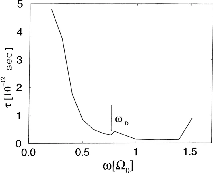
In Fig. 3.3, the dependence of r on 0 is shown. In the graph, the frequencies are given in units of iio· We see that both for large il and small ii, r diverges. For large i) limit, the reason is due to the phase space factors; the two phonons created or absorbed has to be in a band of width 2u}d — H which goes to zero as

ii —> 2o;/5. For n > 2u)o, the adsorbed atom can not decay through the emission

of two phonons and one has to consider three or more phonon processes. In the small i) limit, the coupling constant B becomes very small and the system behaves almost as if it is isolated, and can not decay. In Fig. 3.3, one also sees that in the region fl ~ tup there is a change in r. For i2 < uq there is a contribution to the decay process whereby the adsorbate absorbs a low energy phonon from the sample and at the same time emits a high energy phonon into the sample. This process is absent in the ii > lod case which causes a sharp

change.

E(t)

E(0)

0

E(t)

E(0)

200

300

400

Figure 3.2: Calculated decay profiles, for the energy of the vibrating atom for various i l ’s.

^ Q

3

1

0

0.0

0.5

1

0 )[Q J

1.5

Figure 3.3: Dependence of the relaxation time, r, on the vibrational frequency, fi, of the adsorbate.

C h a p ter 4

C o n clu sio n

We have attacked two different problems using two different methods. In the first chapter, we have used the Keldysh formalism to study the steady state heat current through a ID atomic wire. Its dependence on temperature and the number of atoms is studied. It is found that most of the current is carried by phonons at the eigenfrequencies of the wire. The total thermal conductance is found to be independent of the total number of atoms. However the con­ ductance is smaller for single atom and for N — 2. For > 2, k is stabilized. Note also that we have not considered unharmonic terms within the wires. It is expected that if one allows for phonon scattering within the wire, the current would decrease as one increases the length of the wire, which we expect from our everyday experience. We also observed step in the total conductance as one makes changes in the structure of the reservoir, similar to the steps seen in the electronic counterpart. Hence although one cannot talk about the universal heat quantum as a fundamental constant, heat conductance still shows some kind of a quantized nature. In view of the recent developments, such as the realization of a linear chain between two electrodes consisting of eight atoms, also fabrication of suspended dielectric bridges with nanometer dimensions and also confining a single molecule between two electrodes, put not only academic interest but also the present results will be used in near future, and may con­ tribute to a rapidly developing field, nanoscience. The formalism developed here can be extended to include multiple contacts and in particular to complex molecules between two electrodes.

In the chapter, we studied the dissipation of excess energy, AF^(O), of

an adsorbed atom on a surface and developed a Redfield-Theory like formalism based on the reduced density matrix. We showed that in all cases, the time variation of the excess energy can be fit almost perfectly into the expression

A E { t) = Д£^(0)е“ т^ at Г = 300/i". We calculated the decay rate profiles

and the corresponding relaxation times for various frequencies. Our results are relevant to various theoretical and applied fields including tribology, molecular biology, molecular electronics, and crystal growth.

As regard to the differences in the methodologies in treating these two problems, the Keldysh formalism only gave the steady state properties of the system. It did not yield information about the transient period, i.e. what happens right after we bring the systems into contact. It is not suitable in studying such systems. On the other hand, the Redfield-like approach gave us information about the transient period. The main fundamental reason for this difference is that, in the Keldysh formalism, one directly attacks the calcula­ tion of the expectation value of the operators. But the expectation value of the operators does not specify the state of the system completely. Hence the expectation value of an operator at some time does not give information about it value at following instants. But, in the Redfield theory like approach, the density matrix of the whole system is calculated. As it contains all the infor­ mation about a system, the density matrix at some moment in time determines its value at a further moment, hence it was possible to use an iterative scheme to obtain its evolution for large enough times.

Appendix A

Eq. 2.1

Let O be an operator whose expectation value is to be calculated at time t. Let the system be described by po at time to (later on the limit to —>■ —oo will be considered). Using the Heisenberg equation of motion

TrpoO(t) {0{t)) =

Trpo

(A .l)

where the denominator is substituted for future convenience. Let us consider the numerator only and let (...)o = Trpo·... Then:

where we have seperated the total Hamiltonian as = Tfo + 'Hint- If the operator is differentiated with respect to i, the resultant differential equation can formally be integrated using the boundary condition at i = to- From the uniqueness of the solution, it can be shown that:

where T is the time ordering operator and is defined as:

Similarly:

37

(A.3)

(A.4)

where T is the anti-time ordering operator. Hence we get:

where

Oi{t) = (A.7)

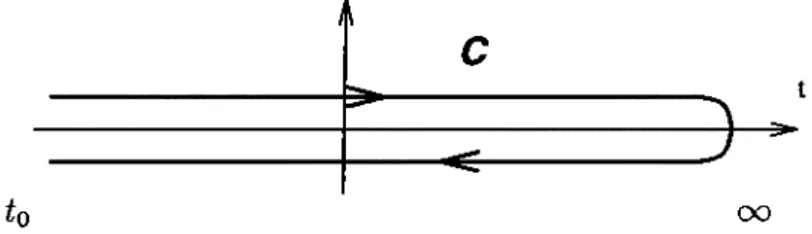
The path ordering operator Tc is defined as the operator which orders the operators in its argument so that if one goes along the time loop shown in the figure below, the operator to the right will be reached later then the operator to the left.

oo

Figure A.l: The time loop along which the operator Tc orders its arguments.

Note that path ordering reduces to time ordering if all the times are on the upper branch and reduces to the anti-time ordering if all the times are on the lower branch. The times on the upper and lower branches will be distinguished by (+) and (“ ) superscripts respectively. Then, Eq. A.6 can be re-written in terms of the path ordering operator as:

(eK«(‘-'o)o(i„)e-K«(‘- ‘o))o = (Tcc"'^'o

(A.8) where we have inserted the identity operator Tee* ) to the left of the operator O. Note that if the time of the operator Oi{t) is assigned the label (+), all the operators in Eq. A.8 are already path ordered. Hence all of them can be written as the argument of a single path ordering operator. Since we can regroup operators within the path ordering operator, we get:

In order to obtain the denominator in Eq. A.l, it is sufficient to replace the operator O in Eq. A.9 with the identity operator. For finite to, the system is not time translation invariant, to fixes a reference time. But this is in general not convenient for calculational purposes. Hence the limit to —oo will be considered. This limit only yields the steady state results. Putting the numerator and the denominator together we obtain Eq. 2.1.

Appendix B

Eq. 2.2 3

First, note that:

m dw .· -oo / 00 ^7/1 — , (B .l) - O O i o T T

where {uL{t)xi{t'))w is the time Fourier transform of (u£,(i)x](F)) = («¿(i — F)xi(O)). Hence if we can calculate this Fourier transform, the current is given by:

Jl = limJL(i)

= - Al [ ^{ - i w ) { u L { t ) X i { t ') ) ^ .

J —00 ioTT

(B.2)

Note that although in Eq. B .l, we used Jl(/) to denote the function, it is not the current at time t.

I will not go into the details of the diagrammatic expansion of correla­ tion functions, and the wick theorem. The diagrammatic expansion for non­ equilibrium systems is identical to the equilibrium case, we only have the additional labels ('^) and (“ ) which should be summed over also (see eg. [29, 30, 31, 32]). For concreteness and simplicity, I will only consider the har­ monic interaction, Eq. 2.16. The Feynman Diagrams will consist of wavy lines,