The Finite Differences Schemes For First Order Nonlinear System Equations In A Class Of Discontinuous Functions

(1)

©BEYKENT UNIVERSITY

THE FINITE DIFFERENCES SCHEMES FOR

FIRST ORDER NONLINEAR SYSTEM

EQUATIONS IN A CLASS OF DISCONTINUOUS

FUNCTIONS

Mahir RASULOV and Bahaddin SÎNSOYSAL

Department of Mathematics and Computing, Beykent University 34396, Sisli-Ayazaga Campus, Istanbul, Turkey

mresulov@beykent.edu.tr bsinsoysal@beykent.edu.tr

ABSTRACT

In this paper a new finite differences schemes of the Cauchy and initial-boundary value problem, for the first order system differential equations which describe some conservation laws is suggested. At first an auxiliary problem which is equivalent to the main problem in certain sense is introduced. On the basis of the auxiliary problem the simple and economical algorithms from computational point of view are proposed.

ÖZET

Makalede bazı korunma kanunlarını ifade eden birinci mertebeden bir boyutlu nonlineer kısmi türevli diferansiyel denklemler sistemi için süreksiz fonksiyonlar sınıfında yeni bir sonlu farklar yöntemi önerilmiştir. Esas probleme denk olan ve bazı avantajlara sahip yardımcı problem içerilmiş ve yardımcı problem kullanılarak sade ve ekonomik sayısal algoritmalar üretilmiştir.

Key Words: Conservation laws, Mathematical modeling of water displacement of oil,

Finite difference scheme in a class of discontinuous functions

1. INTRODUCTION

As usually, let ( x , t) be an element of the space R4, here is

x = ( x1, x2, x3) and t is time and dQ is the boundary surface of Q ^ R3.

It is known that any conservation law expresses by the formula

t2 ^ t2

J p ( x , t ) |

t

jdx + J J A(x,t)ndsdt + Jj>g(x,t)dxdt = 0. (1)

(2)

Here p and g are columns with size 3, A is a vector field of which dimension 3 x 3 , n is a normal vector at any points of dQ . The equation (1) shows that the variation of the set function P ( Q , t) = £ p ( x , t)dx in (t1,12) time

Q

interval, is equal to the variation of A(x, t ) flow which passes over the boundary surface of Q under source function g(x, t) . In general, as the f u n c t i o n p imply a mass, impulse, moment of impulse, energy and etc.

It is known that the state of the system is defined by the speed, pressure and density functions, that are the functions p = p(u, x, t), g = g(u, x, t) , and A = A(x, t) dependent of u = u ( u1, u2, u3) . For the differentiable

u ( x, t) the equation (1) is equivalent to

J J u

_{t, Q}

p

t

+ divA + g )dxdt = 0. (2)

Since the domain Q x ( t , , 12) is arbitrary from (2) we get

p

t

+ divA + g = 0. (3)

The equation (3) can be rewritten in a divergence form as p t + i

f

=

0.

^

dx

j =

G

xJ

In theories, under some assumptions the conservation laws form first order partial differential equations. Hyperbolic systems of first order conservation laws in some space variable has been investigated in [5], and developed an adequate theory of the initial value problem for system of conservation laws.

In this paper we will develop a special differences scheme for system differential equations of conservation laws in a class of discontinuous functions.

2. MAIN AND AUXILIARY PROBLEMS

In the limit of this paper we will investigate the case of n = 1. Let I = (— ro, ro) and R+ = I x [0, T), and we consider the following system of equations

^

Vı

(u, v)

+ f

u v

) =

0

dt dx

(3)

^

< 2

( u , v)

^ f ^ V ^ =

0

(

5

)

dt dx

Here u = u(x, t), v = v ( x , t) are components of u , x is space coordinate and t is time, < ( u , v ) and ft ( u , v ) , (i = 1, 2 ) are differentiable functions

of any coordinates u and v.

Many different problems of physics are modeled by the system equations (4),(5). For example:

I. If < ( u , v) = u, fi(u, v) = uv, <

2

(u,v) = uv, f

2

(u, v) =

uv2 + p(v) then the system equations (4),(5) represent one dimensional,

time dependent constant pressure isentropic of incompressible fluids, [2], [13], [15].

ïï. I f <

=

v , f1

=

-u, < 2 = u , f2 = P O ^

P

( v ) =

kv

-(y > 1, k > 0 are constants) the system equation models the flow of one

dimensional constant entropy incompressible fluids, [2], [13], [15].

III. If

<(h, u) =

h,

f j ( h ,

u )

=

uh,

<

2

(h, u )

= u,

f

2

( h , u )

=

u2

+ gh, then the system of equations (4),(5) describing shallow water flows in an isolated ridge [3], [4], [14].

The initial-boundary value problem for the shallow water equations is investigated in [12]. It has been shown that the solution of this problem has the points of discontinuity of whose the locations unknown beforehand. Since the system (4),(5) are nonlinear, to obtain the exact solution of the Cauchy problem for (4),(5) is impossible, and besides, the Cauchy problem for (4),(5) has not the classical solution.

In this situation, it is necessary to develop a numerical method for obtaining the approximate solution with higher resolvability character. We will investigate the system equations (4),(5) under following initial

u(x,0) = u

0

(x), (6)

v( x,0)

= v 0 (

x)

(7)

conditions. Here, the functions u0 ( x ) and v0 ( x ) are given functions having

compact supports. Later we will call the problem (4)-(7) as the main problem.

2.1. Auxiliary Problem for Cauchy Problem

In this section we will develop a special numerical method for the problem (4)-(7) in a class of discontinuous functions.

(4)

The functions < ( u , v ) and ft ( u , v ) (i = 1 , 2 ) satisfy the following

conditions:

1. <pi ( u , v ) and fi ( u , v ) , (i = 1 , 2 ) are continuous functions for both

arguments u and v;

/ .

d<

2. < ( u , v ) are differentiable functions with respect to u and v, and and

du

d< d t_{do not vanish, the jacobians r— ^ 0 , r— ^ 0 ;} • • b Di<1<2) . 0 P i f ^f2 ) . 0

dv D(u, v) D(u, v)

3. fi, (i = 1 , 2 ) are differentiable and fiu and fiv may change sign.

The weak solutions of the problem (4)-(7) are defined as:

Definition 1. The functions u ( X , t) and v(X, t) satisfying the initial

conditions (6) and (7) are called the weak solution of the problem (4)-(7) if the following integral relations

j j {< (x, t)< (u, v) + f i (u, v)<x }dxdt + J <1 (u

0

, v

0

)<(x,0)dx = 0 (8)

jj{p

t

(x, t)<2 (u, v) + f2 (u, v)<x }dxdt + J<2 (

u

0, v0 )<(x,0)dx = 0 (9)

D -»

hold for every any test functions < ( x, t) which vanishes for sufficiently large

t+|x|.

As it is seen in (8) and (9), the functions u( x, t) and v ( x, t), (even the functions < (u, v) and fi (u, v) , (i = 1 , 2 ) ) may be discontinuous, too.

In order to find the weak solutions of the problem (4)-(7), according to [8], [9], the following auxiliary problem

d p ( x

,

t )

+ f1( x, t) = 0 , (10)

dt

dq( x, t)

+ f2 (x, t) = 0

, (11)

dt

p(x,0) = p

0

(x) , (12)

q( x,0) = q

0

( x)

(13)

is introduced. Here the functions p0 ( x ) and q0 ( x ) are any differentiable

solution of the equations respectively

(5)

= . , ( x ) , ^ = v„(x).

dx dx

Theorem 1. If the functions p(x, t) and q(x, t) are the solutions of the

auxiliary problem (10)-(13), then the functions u ( x , t) and v ( x , t ) defined by

(p

x

(u (x, t), v(x, t)) = M

x

l l ,

dx

cp

2

(u ( x, t ), v( x, t )) =

dx

are weak solutions of the main problem.

2.2. Auxiliary Problem for Initial-Boundary Value Problem

In this section we will investigate the system equations (4),(5) by the initial conditions (6),(7) and the following boundary

u (0, t ) = u

l

(t ), v(0, t ) = v

l

(t )

(14)

conditions. Here u1 (t ) and v1 (t ) are given functions.

In this case the auxiliary problem for (4),(5) is

d

x

— jç>i t), t ) ) = fi (1 (t), vi (t)) - fi (u(x, t), v(x, t)), (15)

Cl

0 d

x

— (u(£, t), v(^, t ) ) = f2 (ui(t), v i ( t ) ) - f 2 (u(x, t), v(x, t)). (16)

Cl

0

The initial conditions for (15),(16) are given in (6),(7). The problem (15),(16) and (14) is called as the second type auxiliary problem, [9], [10].

3. FINITE DIFFERENCES METHOD IN A CLASS OF

DISCONTINUOUS FUNCTIONS

In literature, there are many papers that devoted to study numerical methods for the system equations of conservation laws. In this work, homogenous algorithms (not considering the existence of jump points) for the solutions of equation (4),(6) with suitable initial and boundary conditions are examined [6], [7]. In [11], the difference scheme for solving nonlinear system of equation of gas dynamic problem in a class of discontinuous functions has been studied.

(6)

In order to develop the numerical method, the domain R+ is covered by the grid

Qh T= { ( xt, tk) , xt = ih, tk = kr, dx > 0; i = ...,-n,-n + 1,...,-1,0,1,...,n,...; k = 0,1,...}

here h > 0 and T > 0 are the steps of the grid with respect to x and t, respectively. At any points ( xi, tk ) we approximate the problem (10)-(13) the

following scheme

P i , k + 1 =Pt,k

+Tf1

(

U,

k ,Vl,k

)

( I7)

Qik+1 = Qik + T f2 (U,,k ,V , k) , (1 8)

P i , 0 = p0( xi), ( I9)

Q,

,0 =

q

0

( x).

(2 0)

The finite differences scheme (17)-(20) is an explicit, and it is known that for sufficiently small T , this scheme gives correct results.

For the problem (10)-(13) we can write the implicit scheme as

P i , k + 1 = P i , k - T f 1 ( Ui , k + 1 , P i , k + 1 ) , ( 2 1 )

Qi,k+1 = Q i , k T f2 {UlM1,VlM1 ). (2 2)

The initial conditions for (21),(22) are given in (19) and (20). Using the Newton iteration method we can obtain the solution of the nonlinear algebraic equations (21),(22). Here pik, Qik, Uik , and Vik denote the

approximate values of the unknown functions

p(x,t), q(x,t), u(x,t),

and v ( x, t) at the point ( xi, tk ) e Q h T.

Theorem 2. If pik+1 andQik+1 are the numerical solution of the problem

(17)-(20), then the functions Uik+1 and Vik+1 obtained by

<1 (U,k+1,V,k+1) = Pxx , (2 3)

< ( U „ k + 1 , V , k + 1 ) = Qx (24) are the numerical solutions of the main problem.

Applying the Runge-Kutta method to the problem (21),(22), we can get a higher order finite-difference scheme for the main problem with respect to T .

3.2. Numerical Algorithm for Initial-Boundary Value Problem

In order to approximate the problem (15),(16) and (14) by finite differences scheme at any points ( xi, tk ) of the grid Q T , we will use the following

(7)

J f

(£,

ty% =

h ¿ Fjk (25)

0 j=1

formula. Taking (25) into consideration, the system equations (15) and (16) are approximated a

pp~ (U,k, Vhk+1 )U, k+1 + pp~ (Uhk, Vk )Vuk+1 = I + (p[~uhk + V,k, (2 6)

<p2~~(ua ,V.M1)U1M1 +p2~(u,,k ^ )V,k+1 = I + p 2 v U , , k + p 2 v V , k , (2 7)

where I « = ~rfv ( " 1 (tk), V1 ( t k ) ) -- T

f

v ((, k , V , k ) h

h

- Z pu ( + 1 , Vjk+1)- Pu( , j ^ (28) j=1 ( u = 1 , 2 ) a n d

pUv

a n d

PUV

a r e p U V )= p ( u , k i ,k+1 p1 V u i ,k , Vi , k + 1 / = TT TT ' ui , k + 1 - U,,k P U V )= P( Ui , k i , k +1) - P ( u, , k ,V,k+1 ) p 2V Ui , k , Vi , k + 1 / = T / ' V,k+1 - V,k

here, Ui k e ( u , k , U i,k+1₎_,_V_',k_{e (V}_i,k_{, V}_,k+1₎_._{S i n c e t h e}_j_{a c o b i a n}

Dp, p

2

)

= 0 , is not equal to zero we can find the explicit expressions for

D(u, v)

U, k+1 and Vi k+1 from (26),(27), respectively.

4. APPLICATION THE SUGGESTED METHOD TO

THE PROBLEM OF OIL DISPLACEMENT WITH

CHEMICAL ACTIVE MIXTURE

In order to demonstrate the efficiency of the suggested method we have applied this method to the problem which describes the process displacement of oil by the chemical active solvents (surfactant polymer, etc.)

It is known that in the state of thermodynamic equilibrium, in which capillary pressure is neglected , then one dimensional system equations that describe the large scale process of oil-water displacement, takes the following form

(8)

da . . dF

1

(a, c)

n m + w(t)—1V y = 0,

dt dx

m ^ O f l + w(t)

d F2(ac )

dt dx

= 0.

(29) (30) Here F1 ( a , c ) , F2 ( a , c) and G ( a , c) are given functions as

Kw (a, c)

F

1

(a, c) = ,

Kw ( a , c ) + juK0(0, c) F2 ( a , c )

=

Fi c ) c

+

[ l - Fi ( a , c )

R

c )

a

(

v)

m

G(a, c) = ac + (1 a)p(c) +

-Uw (c) = 1 + 0 . 5 4 - 0 . 3 ( 4

c v c

U ( c ) = 1 4 . 5 - 1 4 . 7 4 + 5.5|-

c r

c

V

c

,

, u = Uwic)

U 0( c )

c * = 0.086,

The Buckley-Leverett's functions are expressed as

Kw

(a,

c) =

0,

( a - 0.2'

V 0.8 ,

a <

0.2 a > 0.2,

K0(a,c)=

a >

0.83

0.74

<

a

<

0.83

( 1 - K22 ) +

K2,

a <

0.74,

K 2C 2

C 2 =

(P(c)

Kc *

, cp(c)

=

Kc , K

=

2, a ( a )

=

0,

K 1 =

0.83 - a

_{K 2 =}

0.74 - a

0.834 ^ ^ 0.715 )

m

=

0.2, w(t)

=

3.016

x

10

-5

.

Here Kw ( a , c ) , K0 ( a , c ) denote partial permeability of water and oil

phases respectively; F1( a , c ) , F2( a , c ) , which determine water and oil

fractions in the total volume of fluid of the mixture are called Buckley-2

2

3

(9)

Leverett's functions; a ( c ) - the mass of absorption of active solution in per unit volume of the porous medium; (p(c) - the mass concentration of the active solution in the water and oil phase; fiw(c), ¡u0(c) dynamical

viscosity of water and oil respectively; m - porosity; c - saturation of water phase; c - concentration of mixture in water phase.

The initial and boundary conditions for (29),(30) are

c(

x,0)

=

c

0

( x)

=

0.2, c( x,0)

=

c

0

(x)

=

0,

(31) f

1, 0

<

t

<

T

0

c(0, t)

=

C (t)

=

0, c(0, t)

=

ci(t)

= j 0 t 0 (32) [ 0

,

t > T0 .

Here, T0 is the pumping time of chemical active water into the porous

medium.

In order to approximate the problem (29)-(32) at first, we introduce the second type auxiliary problem as

x

m\a(£, t)d$ + w(t)Fi (c(x, t), c(x, t)) = w(t)F ( (t), c (t)) (33)

0

m j

G ( t), c(£ t))) +

w(t

)F

2

(c( x, t), c( x, t)) =

w(t

)F

2

( ( t ) ,

ci

(t)).

( 3 4 ) 0

Using (25), the system equations (33),(34) are approximated as Z ik+i = Z ik + Tw ( tk ) F1 ( i ( tk X ci ( tk ) )

-- T w ( t

k

) F i ( Z i , k , C , , ) - Z ( Z M+1 - Z M ) (35)

n

j=i CA + 1 = C A + [ GC ] 1

T w(tk )F

2

( (t

k

),

cI

(t

t

)) - T w(t

k

)F

2

(Z ik, C

hk

)

-n -n

Z [

G

(Z j,k+i

, C

jk+i

) - G

( Z jk

, C

j k

) ] - G

C (Z ik+i

-

Z ik )

j=i

. (36)

dG

Here G~ is the value of at the time layer t = tk . Using the difference

C

dc

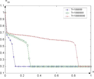
scheme (35),(36) computer experiments has been carried out and the results of the experiments are demonstrated in Figure i and Figure 2.

(10)

5. CONCLUSION

In this paper an original numerical method for finding the weak solution of the initial and initial-boundary value problems for first order system of nonlinear partial equations in a class of discontinuous functions is developed. Suggested method has been applied to the displacement of oil process by the chemical active mixture in porous medium.

1.1 1 0 . 9 0 . 8 0 . 7 0 . 6 0 . 5 0 . 4 0 . 3 0 . 2 0 . 1 0 . 2 0 . 4 0 . 6 0 . 8

Figure 1. Dynamical distribution of water saturation

0 . 0 6 0 . 0 5 0 . 0 4 0 . 0 3 - 0 0 . 0 2 -0 . -0 1 0 0 0 . 2 0 . 4 0 . 6 0 . 8 1

Figure 2. Dynamical distribution of concentration

0

(11)

REFERENCES

[1]. Anderson, D. A., Tanrehill, J. C., Pletcher, R. H., Computational Fluid Mechanics and

Heat Transfer, Vol. 1,2, Hemisphere Publishing Corporation, 1984. [2]. Courant,R, Friedrichs,K.O. Supersonic Flow and Shock Waves,

Springer-Verlag, New York,1976.

[3]. Houghton, D. D., Kasahara, A., Nonlinear Shallow Fluid Flow Over an Isolated Ridge, Comm. Pure and App. Math., Vol XXI, (1968), pp.1-23. [4]. Korteweg de- Vries G. On the Change of Form of Long Waves

Advancing in a Rectangular Channel and on a New Type of Long Stationary Waves. Phil. mag., v.5, No:39, (1895), pp.422-443.

[5]. Lax, P. D., Hyperbolic Systems of Conservation Laws II, Comm. of Pure and App. Math., Vol. X, (1957), pp 537-566.

[6]. Liska, R., and Wendorf, B., Composite Schemes for Conservation Laws, SIAM J. Num. Anal., 35 (1998), pp. 2250-2271.

[7]. Noh, W. F., Protter, M. N., Difference Methods and the Equations of Hydrodynamics, Journal of Math. and Mechanics, Vol.12, No.2, (1963). [8]. Rasulov, M. A., On a Method of Solving the Cauchy Problem for a First

Order Nonlinear Equation of Hyperbolic Type with a Smooth Initial Condition, Soviet Math. Dokl. 43, No.1, (1991) pp.150-153.

[9]. Rasulov, M. A., Finite Difference Scheme for Solving of Some Nonlinear Problems of Mathematical Physics in a Class of Discontinuous Functions, Baku, 1996, (in Russian).

[10]. Rasulov, M. A., Karaguler T., Finite Difference Scheme for Solving System Equations of Gas Dynamic in a Class of Discontinuous Functions, App. Math. and Comp.143

(2003), pp. 145-164.

[11]. Rasulov, M.A., Karaguler, T., Sinsoysal, B., Finite Difference Method for Solving Boundary Initial Value Problem of a System Hyperbolic Equations in a Class of Discontinuous Functions, App. Math. and Comp.149 (2004), pp. 47-63.

[12]. Rasulov, M. A., Aslan, Z., Pakdil, O., Finite Differences Method for Shallow Water Equations in a Class of Discontinuous Functions. App. Math. and Comp. 160 (2005), pp. 343-353, 2005, USA.

[13]. Smoller, J. A., Shock Wave and Reaction Diffusion Equations, Springer -Verlag, New York Inc., 1983.

[14]. Stoker J.J. Water Waves. Inter science Publishers, INC., New York, 1957.

[15]. Whitham, G. B., Linear and Nonlinear Waves, Wiley Int., New York, 1974.