Environmental Sustainability Target. Evidence from Europe Largest States
Andrew Adewale Alola
Faculty of Economics, Administrative and Administrative and Social Sciences, Istanbul Gelisim University, Istanbul, Turkey.
Email:[email protected]
Kürşat Yalçiner
Faculty of Economics, Administrative and Administrative and Social Sciences, Istanbul Gelisim University, Istanbul, Turkey.
Email:[email protected]
Uju Violet Alola
Faculty of Economics, Administrative and Administrative and Social Sciences, Istanbul Gelisim University, Istanbul, Turkey.
Email:[email protected]
Seyi Saint Akadiri
1Faculty of Business and Economics, Department of Economics, Famagusta, Eastern Mediterranean University, North Cyprus, via Mersin 10, Turkey.
Email: [email protected]
Abstract
In spite of the continued deployment of technologies, innovations toward addressing the
challenges of global warming, forecasting and sustaining quality environment have remained the
herculean endeavour of the advanced states. Also, being migrants’ destinations, resulting from
the availability of economic opportunities, the target of attaining low-carbon, energy efficiency,
and the cleaner atmospheric environment by these advanced economies are further bewildered.
In that light, we investigate the impact of renewable energy consumption and migration on the
1
Faculty of Business and Economics, Department of Economics, Famagusta, Eastern Mediterranean University, North Cyprus, via Mersin 10, Turkey.
*Corresponding: [email protected]
carbon dioxide emissions of the panel of EU’s largest economies of France, Germany, and the
United Kingdom over the period of 1990 – 2016. The consistency of the Group FMOLS and
DOLS presents elasticity of -0.13 and -0.14 respectively for the nexus of renewables and CO2.
Similarly, 0.04 and 0.05 are the respective elasticity of the two models for the nexus of migration
and CO2. In support of extant literature, the nexus of CO2 with GDP and CPI are significant, and
respectively positive and negative. In addition, the study reveals evidence of Granger causality
with feedback between renewable energy consumption and CO2, and between CPI and CO2. On
the other hand, a unidirectional Granger causality running from migration to CO2 is observed. In
practical term, the study presents policy frameworks for the examined countries and other
advanced nations. The implementation of the presented policy pathways are potentially geared
toward a forecastable, sustainable environmental quality and energy efficiency targets.
Keyword: Environmental quality; Carbon emissions; renewable energy consumption; migration; France,
Germany, United Kingdom.
1. Introduction
In recent years, energy technologies, innovations are some of the ploy that are directly targeted at
reducing carbon dioxide emissions or in general the greenhouse gas. Across the globe, there have
been relentless efforts toward mitigating the adverse effect of global warming, climate change,
desertification, land degradation, and related human-environmental and ecological distortions.
Carbon emissions have persistently become the world’s most threatening issue facing the natural
ecosystem and human development. This is the reason population-environment system (PES)
which is mainly constituted by the dynamics of fertility, mortality, migration, and other social
and economic factors cannot be exonerated from global challenge facing the ecosystem (Han et
Panel on Climate Change (IPCC, 2014) reported that carbon emission has undesirably increased
from 9434.4 million tons in 1961 to 34649.4 million tons in 2011. The Co2 emission (most
common greenhouse gas, GHG) primarily constitutes about 81% of the GHG, thereby
responsible for the global climate change. In the report of the British Petroleum (BP) Statistical
Review of World Energy (BP, June 2018), it mentioned that carbon dioxide emissions increased
from 29714.2 million tons in 2009 to 33444.0 million tons in 2017. In spite of the Paris
Agreement of 20152 and the strong drive toward reducing carbon emission by countries, the
aforesaid report indicates that the global carbon dioxide emissions increased by 1.3% between
2006 and 2016, and also increased to 1.6% in the previous year (2017). Also, in the period
2007-2017, the growth rate of carbon dioxide emissions in the European region is about 2.5% and was
reportedly the second highest globally.
In recent time, most developed countries have continued to experience significant declining
growth rate in the volume of carbon dioxide emitted. For instance, 4152.2 million tons (third
highest volume) of carbon dioxide is emitted by the European countries in the period 2007 to
2017 (BP, June 2018). As constituents of the aforesaid volume of emitted Co2, the volume of the
emission is higher in the order of Germany (763.8 million tons), United Kingdom (398.2 million
tons), Italy (344 tons), and France (320.3 tons). Surprisingly, Germany with the highest volume
of Co2 is observed to have a growth rate of 0.1% in the same period 2007 to 2017. While the
growth rate of Co2 emission in France is highest (2.0%) among the countries, the United
Kingdom record the lowest growth rate of -2.7% in the same period. Generally, human activities
and other unavoidable factors have significantly contributed to the increasing volume of carbon
dioxide in most advanced countries through the disruption of the carbon cycle.
2
More details relating to the Paris Agreement of 2015 is contained is available at: https://unfccc.int/process/conferences/pastconferences/paris-climate-change-conference-november-2015/paris-agreement.
In turning down the heat i.e cutting down carbon emissions in these countries and in other large
economies of the world, countries have intensified the development of efficient energy source.
For instance, three of the aforementioned countries; France, Germany, and the United Kingdom
have shown a considerable increase in the development of renewable energy. In 2017, Germany
invested about $10.4 billion in renewable energy (the highest in Europe), followed by the United
Kingdom with $7.6 billion, thirdly by Sweden with $ 3.7 billion, and France with $2.6 billion
(United Nations Environment Program, UNEP, 2018). Resulting from this investment, thousands
of Megawatts of renewable energy sources was generated to produce electricity during the
previous year 2017. For instance, the renewable power capacity which represents the maximum
net generating capacity of power plants and other renewable energy installations for Germany,
France, and the United Kingdom respectively produced 113, 058 Megawatts, 46, 678 Megawatts,
and 40, 789 Megawatts electricity in 2017 (International Renewable Energy Agency IRENA,
2018).
Another dimension to this since the Second World War is migration (the movement of people
from one location to the other with a motive of permanently or temporarily residing in the new
location) and has continued to be a challenge across the globe. Generally, these movement of
people is largely attributed to high and increasing population pressure on the scarce resources
(Alola, 2019; Ma, & Hofmann, 2018; Alola & Alola 2018a).In Europe, the relocations of people
(legally or illegally) that includes asylum seekers, refugees and migrants was peaked in 2015 to
2016 in Europe at yet the highest level since spillover effect of the Second World War. The
concern associated with the record experience during the time period mentioned earlier is not
unconnected with the irregular immigration of people from outside the European Union (EU)
en route the frontline Southern countries (Italy, Greece, Malta, e.t.c. are frontlines countries), and
the hardline Central and Eastern European states (Poland and Hungary are examples), their major
target countries are the more prosperous Northern European countries (these include France,
Germany, and the United Kingdom). Importantly, since 2015 Germany who has received the
highest number of asylum seekers and other migrants have recently considered a retrospect of its
approach likewise France and the United Kingdom. The multiplicity of problems;
socioeconomic, environmental, and among other challenges associated with this movement of
people have triggered discuss on wider border control and migration policy across the EU.
On this note, the current study is designed to underpin the trilemma of the simultaneous
frameworks of the development of renewables, migration policy and real income considering the
growing trend of energy demand and decarbonization agenda of the advanced economies. The
study hypothesize the impacts of renewable energy consumption,migration policies, and the real
income on the environment quality vis-à-vis carbon emissions of France, Germany, and the
United Kingdom. The approaches of Fully-Modified Ordinary Least Square (FMOLS) and the
Dynamic Ordinary Least (DOLS) are engaged in the investigation over the time period 1990 –
2016. Although previous studies employed the panel studies of categorization of the EU
countries using varieties of methodologies (Karmellos, Kopidou & Diakoulaki, 2016; Moutinho,
Madaleno & Silva, 2016; Soytas & Sari, 2009), the specifics of the novelty of the current study
seeks to close notable gap in extant literature accordingly:
• The examined panel countries that include France, Germany, and the United Kingdom have rarely been investigated in a panel study at least within the current context. Being
economic characterization in relation to approaches toward attaining efficient energy and
meeting their respective low carbon targets makes this an informative study.
• Also, the reason for switching from high-carbon energy to alternative energy like the renewables is mainly to cut back the effects of global warming associated with the
greenhouse gases. The desire to meeting the above objective by France, Germany, and
the United Kingdom have over time contended with yet another inhibiting factor, the
potential challenges posed by forms of migration. Hence, investigating the response of
the carbon emissions level to the intrigues associated with the development of renewable
energy, immigration policy, and real income dynamics in the panel countries is posed to
divulge interesting and uncommon empirical interpretation. The aforementioned potential
environmental quality determinants are akin to the innovation polies employed in the
study of Fernández-Sastre & Montalvo-Quizhpi (2019).
• Lastly, by employing the Granger causality of Dumitrescu and Hurlin (2012) to underpin the interaction between the observed factors, it study tends to reflect a unique
underpinning of historical information and adds to the body of existing literature.
The rest of the sections are in part. The next section (2) contains a synopsis of the previous
studies. The materials and methodologies employed are presented in section 3 while the results
are discussed in section 4. Section 5 offers concluding remarks that include policy implication of
the study and proposal for future study.
2. Background: A synopsis
In tackling the global challenge of climate change, the European Union has reaffirmed its
position and commitment toward attaining a sustainable environment. The focus is to reduce
of climate change. Although the EU have over-achieved its earlier CO2 and greenhouse gas
reduction commitment within the first period of the Kyoto Protocol (2008-2012), further targets
were being set to compliments ongoing researches on the subject. In the literature and in recent
time, the emission of carbon dioxide in the developed countries (like the France, Germany, UK,
US, and even China) has continued to be associated with varieties of factors (Akadiri, S. S.,
Alola, A. A & Akadiri, A. C., & Alola, U. V. (Forthcoming); Ahmadalipour et al., 2019; Ma &
Hofmann, 2018; Atinkpahoun et al., 2018; Alola & Alola, 2018b; Aunan & Wang, 2014).
In a recent study, Bekun, Alola and Sarkodie, 2019 examined the nexus renewables,
non-renewable energy, natural resource rent, and environmental sustainability for sixteen selected EU
countries. Bekun, Alola and Sarkodie (2019) employed the Pooled Mean Group (PMG) approach
with an Autoregressive Distributed Lag (ARDL) for the period 1996-2014 and found that
renewable energy consumption in the panel countries favours the environmental sustainability
goals and energy policies of the examined countries. Interestingly, it suggests that these countries
are on right pathway mechanism toward achieving the Sustainable Development Goals (SDGs)
2030 especially through their energy diversification policies. On the other hand, the study posits
a long-run negative impact of both economic growth (an indicator for growth in real income) and
natural resource rent on environmental sustainability. This implies that the economies of the
panel of EU-16 countries (among are France, Germany, and UK) are expected to grow at the
expense of their environmental quality. Although both economic growth and the natural resource
rent are observed to negatively impact the quality of the environment in these countries, the
impact of the consumption of the fossil fuel is observably more damaging. On a general note, the
aforementioned results has little or no deviation from the study of Karmellos, Kopidou and
2019; Dong, Jiang, Sun & Dong, 2018; Nguyen & Kakinaka, 2018; Duman & Kasman, 2018;
Kasman & Duman, 2015; Lu, Lin & Lewis, 2007).
Specifically, Karmellos, Kopidou and Diakoulaki (2016) investigated the EU-28 by adopting the
Log Mean Divisia Index (LMDI) method for the decomposition analysis of CO2 emissions from
electricity generation of the EU-28 countries during the period 2000 – 2012. The LMDI method
employed in the study provides decomposition without residual terms and is consistent in
aggregation as such that is capable of computing zeros and negative values. In the study, the
driving factors of CO2 across EU-28 reflects the major policy frameworks underlying the EU
approach to sustainable development. These factors include the activity effect (economic
performance indicator), the electricity intensity effect (ratio of total electricity consumption to
total GDP), the electricity trade effect (ratio of electricity production to electricity consumption),
and the energy efficiency effect (ratio of fuel input to the respective electricity output). Among
the factors enumerated above, the activity effect is observed as the main factor contributing to
the change in CO2 emissions in all the estimated panel countries. Carbon dioxide emissions were
also observed to increase by 12% during the period 2000 - 2007 in 22 of the 28 estimated
countries.
Furthermore, similar to the study of trade-monetary-immigration nexus and the environmental
sustainability of the US by Alola (2019), Han et al (2018) examined the dynamics of migration
and particulate (PM2.5) in China. The concern of particulate pollution resulting from population
change which is strongly induced by rapid urbanization in China has propelled the study of Han
et al (2018). Han et al (2018) identified the important role of migration in urbanization, thus
developing Chinese regions. In the study, the PM2.5 was employed to proxy for environmental
pollution and thus establishing a strong relationship between the observed variables. The study
found that increased population density (especially in Eastern China, Western China, and the
country’s high population density regions) implies increase in the PM2.5 over the period
2000-2014. The implication of the study of Han et al (2018) is a needful call on countries to design
urbanization strategic plan especially that address the forms of migration in order to mitigate the
risks of environmental degradation. In the study of the immigration/migration-environmental
sustainability nexus, the observation from Han et al (2018) and Rafiq, Nielsen and Smyth (2017)
slightly differs from that of Ma and Hofmann (2018) and Aunan and Wang (2014). In specific,
Ma and Hofmann (2018) observed a weak link between immigration and environmental quality.
Rather, the study posits that native population causes more environmental pollution that the
immigrant population in the US. But the study hinted that the tendency of immigrants in
improving the air quality would largely depend on the country of origin of the immigrants. While
Aunan and Wang (2014) noted that rural-urban migration across most Chinese provinces have
significantly reduced the population exposure to PM2.5 especially because of the expected change
in the peoples’ lifestyles, Rafiq, Nielsen and Smyth (2017 noted otherwise for inter-provincial
migration and for SO2 pollutions in China.
Moreover, handful of European countries-specific and related studies have also been conducted
in recent time (Cooper, Stamford & Azapagic, 2018; Cansino, Román & Ordonez, 2016;
Robaina-Alves, Moutinho & Costa, 2016; Baiocchi, Minx & Hubacek, 2010). Specifically for
the United Kingdom, Cooper, Stamford and Azapagic (2018) recently observed that the
development of shale gas in the UK especially for the future energy scenario (toward 2030) is
that lower share of shale gas in the country’s electricity mix of 2030 is more sustainable. Also for
the UK, Baiocchi, Minx and Hubacek (2010) emphasized that carbon dioxide emissions in the
country vary directly and indirectly with the consumer behaviour of different lifestyles of the
consumers as well social factors associated with the people. On different notes, Cansino, Román
and Ordonez (2016) and Robaina-Alves, Moutinho and Costa (2016) respectively investigated
the drivers of carbon dioxide emissions in Spain and Portugal by both applying a decomposition
analysis. While the former examined carbon dioxide emissions in a six-sectoral levels analysis,
the later investigated the contribution of Portuguese tourism sector to carbon dioxide emissions
over a different period of time.
3. Materials and Methods
3.1 Description of MaterialsA multivariate approach is adopted in this study by incorporating four explanatory variables of
annual dataset spanning from 1990 to 2016. The two main independent variables deployed are:
• The renewable (ren, is the final renewable energy consumption measure in Million tons of energy, Mtoe) from the European Commission (EU, 2018) and
• The migration index (mgr, it is an indicator for the movement of people within a territory which proxy for the immigration policy). The migration indices are the policy categories3
which comprises the ranges of sub-indexes from news data. Information from the
employed news categories is derived from the Access World News database of thousand
newspapers which were categorically normalized into series and made available online
(http://www.policyuncertainty.com/categorical_epu.html).
3
More details on the US Policy categorical indices are available at http://www.policyuncertainty.com/categorical_epu.html.
Other independent variables of interest are the consumer price index (cpi) from the World
Development Indicator of the World Bank database (WDI, 2018) and the Gross Domestic
Product (GDP is the Mrd, billion Euro at current price) from the European Commission (EU,
2018). These variables, CPI and GDP are appropriately employed in this study to account for
other unobserved factors to avoiding possible biases caused by an omitted variable. Specifically,
the selection of the GDP gives a trend of the economic growth of the countries while the CPI
captures the effects associated with consumer items that include energy technologies.
Also, the European Commission (EU, 2018) is the source of the dependent variables employed
i.e. the total Carbon dioxide (C02) emissions and the Greenhouse gas (GHG) which are
equivalent of Million Tons of Carbon Dioxide including international aviation. The descriptive
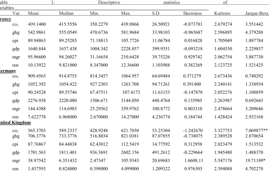
statistics are implied in Table 1.
<Insert Table 1 here>
3.2 Methodology: theoretical concept
Several guidelines for estimating direct C02 emissions have been applied in extant literature over
time (Al-Mulali, Tang & Ozturk, 2015; Farhani & Ozturk, 2015; Wang & Zhao, 2018 Yu, Deng
& Chen, 2018). Here, our study incorporates migration index (mgr) in lieu of health expenditure
in addition to renewable energy consumption (ren) in the recent work of Apergis, Jebli &
Youssef (2018) and allows Gross Domestic Product (GDP) and consumer price index control for
unobserved factors. Hence, the panel empirical expression under investigation is given as:
Co2 i,t = f (gdpi,t, cpii,t, reni,t, migration,t) (1)
Then, the natural logarithmic transformation of the above expression (equation 1) is given by:
for all t = 1990,…, 2016, i = 1, 2, and 3 (respectively for France, Germany and the United
Kingdom). And, βs are the degree of response of the logarithms of the explanatory variables to
the logarithms of Co2 given that εis iiid ~ N (µ, σ2) for every i and t.
3.2.1 The panel unit root tests
In the meantime, we engage the panel unit root test by Im, Pesaran and Shin (IPS, 2003) because
of advantage in modelling both cross-sections and balanced panel data that possesses identically
distributed variance and mean of error terms (as in the case of the investigated countries, France,
Germany, and the United Kingdom). Generally, the method uses the evidence on unit root hypothesis from N unit root tests to examine through DF or ADF regression4 based on the N
cross-section units of the aforementioned variables y as expressed below:
yi,t = α i + ρi yi,t-1 + ε i,t
where t = 1, 2, …, T, null hypothesis (H0) against the alternatives (H1) are respectively given as:
H0 = ρi = 1, ∀ i = 1, 2, …, N
H1 = ρi ˂ 1, ∀ i = 1, 2, …, N1; ρi = 1, ∀ i = N1 + 1, N1 + 2, …, N
Similarly, both the Levin, Lin & Chu, (LLC, 2002)5 and the Fisher-Augmented
Dickey-Fuller/Phillips-Perron panel unit root method, as modified by Maddala and Wu (1999) and Choi
(2001) from Fisher’s (1932) are additionally employed. The step-by-step procedure is skipped
here due to page constraint.
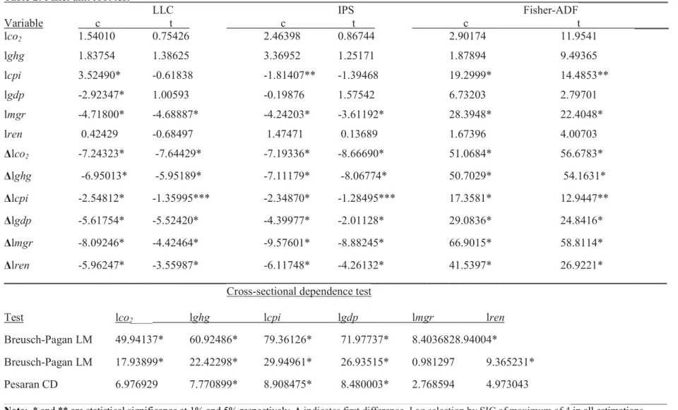
The panel unit root test results from the three aforesaid methodologies are presented in Table 2.
<Insert Table 2>
3.2.2 The cointegration estimation
4
Because of space constraint, the detail and step by step procedure of panel unit root test by IPS and Fisher-ADF/PP are respectively provided by Im, Pesaran and Shin (2003) and Maddala and Wu (1999)
5
A pre-test to investigate panel cointegration evidence by Pedroni residual and Kao (1999) are
essentially employed before using the FMOLS and DOLS estimators. The tests affirm strong
evidence of cointegration in the panel as depicted in the upper part of Table 3.
In this investigation, the Fully-modified ordinary least square (FMOLS) and dynamic ordinary
least square (DOLS) estimators are employed as to overcome the challenges of endogeneity in
the series and the serial correlation issue from the error term. While the FMOLS (an
asymptotically unbiased estimator) employs the semi-parametric correction approach to
investigate the long-run relationship of Phillips and Hansen (1990), Saikkonen (1992) and Stock
and Watson (1993) modelled with a more efficient asymptotic estimator. Given the idea of a
fixed effect model, the equation 2 could be expressed as:
lco2i, t = αi + β x i,t + εi, t (3)
given that for every i = 1 to 3 (i.e i=1 for France, i=2 for Germany, and i = 3 for the United
Kingdom), t = 1, 2, …, T for all series. αi are intercepts for the cross sections, εi, t are stationary
disturbance terms. Also, given that x i,t are the vector of independent variables (lgdp, lcpi, lren,
and lmgr) such that β is the vector of parameter for each x i,t, the autoregressive form is
x i,t = x i,t-1 + εi, t. (4)
Hence, the basis of the model will be to estimate the panel cointegrating vector β, this is obtained
from
FMOLS = { ∑ ∑ , − , − }-1 * { ∑ ∑ , − ℎ , − ∆ ε u
} (5)
but, augmenting the cointegrating regression using lag and lead difference of the independent
variables (lgdp, lcpi, lren, and lmgr) with the DOLS approach, we then have
Also, in Table 3, the remaining information in the lower part contains the results of the
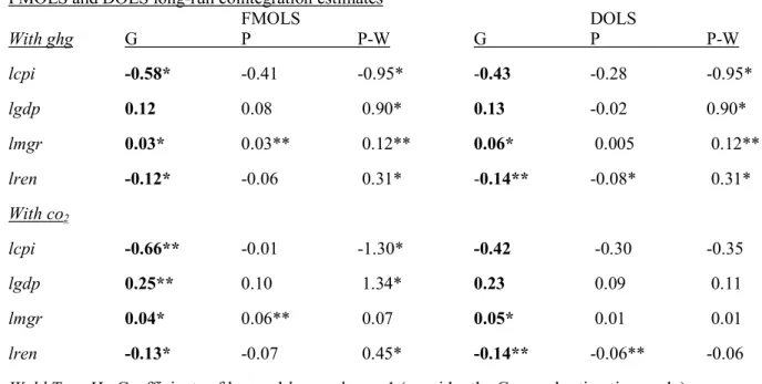
above-mentioned estimations.
<Insert Table 3>
3.2.3 Dynamic Granger causality
Given the asymptotic distribution vis-à-vis the value of T (27) to be greater than N (3), the panel
Granger causality approach by Dumitrescu and Hurlin (2012) for heterogeneous non-causality, is
appropriately employed using the expression below:
Co2it = ' + ∑)( ( 2, #( + ∑ * ( )
( , #( + +, (7)
The fixed effect denoted by ' is neglected in this case as the equation implies a Granger
causality from x to co2 where x = f (lgdp, lcpi, lren, and lmgr) i.e each of the independent
variable. Also, the above expression possess the potential of estimating in a two-directional
manner for a pair of estimated variables with lag length R, It further shows that ( is the
autoregressive parameter (coefficient of the lag of the dependent variable) while * ( is the
repressor coefficients for each estimates. Because Granger causality test assumes a
heterogeneously normal distribution, a homogenous non-stationary (HNC) employed for the
hypothesis testing is illustrated as:
H0 = γi = 0, ∀ i = 1, 2, …, N
H1 = γi = 0, ∀ i = 1, 2, …, N1; γi ≠ 0, ∀ i = N1 + 1, N1 + 2, …, N
given that γi = (* , …, *)), N1 = N indicates that causality of any member of the panel but N1 = 0
indicates causality within cross-sections as the value N1/N is reasonably less than one. The
estimate of the Granger causality test is presented in Table 4.
3.3 Robustness and diagnostic tests
The robustness of the outline-above for appropriateness by re-modeling equation (1). By
replacing the carbon dioxide emissions (CO2) with the Greenhouse gas emissions (GHG) of the
equation (1), a robustness check is performed by using,
l GHG i, t = α + β1l gdpi,t + β2 l cpii, t + β3l reni, t + β4l migration,t + εi, t (8)
The check procedures include a replicated FMOLS and DOLS methods earlier described
Given the observation from the aforesaid re-estimation (also see Table 3), the result further
support the suitability of the methodological concept adopted.
Furthermore, the residual tests of both serial correlation Langrage multiplier and
heteroskedasticity tests found strong significant evidence of no serial correlation and very weak
evidence of heteroskedasticity (see the upper part of Table 4 above)
<Insert Figure 1>
<Insert Figure 2>
4. Results and Discussion
During the time period 1990 – 2016, as depicted in the descriptive Table 1, the estimated
statistics offers useful empirical inference. The results indicate that carbon dioxide emissions and
the greenhouse gas in Germany and the United Kingdom are significantly more than the
emissions obtainable in France. In the same vein, renewable energy was less consumed in
Germany and the United Kingdom. For instance, while Germany recorded maximum CO2 and
GHG of 1064.957 and 1263.708 respectively against 439.8868 and 581.9684 for France, the CO2
and GHG in the United Kingdom is peaked at 621.7030 and 821.058 against the aforementioned
for by the disparity in the volume of renewable energy consumed across these countries over the
same period. In France, 8.347000 Mtoe was the minimum renewable energy consumed, while
2.670000 Mtoe and 0.398000 Mtoe of renewables were consumed in Germany and the United
Kingdom respectively. Specifically, in Germany, the growth rate of renewable energy consumed
in the observed period is significantly higher while the migration index (rate of potential
migration) was also highest. And, this is obtainable in the current reality of both the alternate
energy use the migration policy in Germany. By intuition and economic logic, the observed
economic growth (an indication of more economic activities) in Germany and the United
Kingdom during the investigated period largely accounts for the massive increase in the carbon
dioxide and greenhouse gas emissions. Although the renewable energy of the two countries
(Germany and UK) were lower than that of France at some point, the use of other energy source
especially the fossil fuels would likely be the driver of these economies at such instance. The
behaviors indicates a partial heterogeneity (see Table 2).
On the nature of the relationship between the variables in the model, statistical evidence shows
that the null hypothesis of no cointegration is rejected by the Pedroni Residual and Kao residual
Panel Cointegration methods. An additional test to support the evidence of cointegration (long
run) relationship was employed and the result indicated in Table 3. Also, the long-run
cointegration estimates from the Fully-modified ordinary least square (FMOLS) and dynamic
ordinary least square (DOLS) are presented. In adopting the FMOLS and DOLS approaches, the
Pooled, Pooled weighted, and the Grouped Mean of both estimators were employed. As observed
in the long-run relationship estimates of the explanatory variables and the independent variables
are more consistent with the Grouped mean estimates. Therefore, the elasticity of the carbon
product, and the consumer price index are respectively -0.13, 0.04, 0.245, and -0.66 using the
FMOLS. Similarly, DOLS indicates that the elasticity of carbon dioxide emissions with respect
to the renewable energy consumption, migration, gross domestic product, and the consumer price
index are respectively -0.14, 0.05, 0.23, and -0.42. In both cases, the elasticity coefficient of
renewable energy consumption and the consumer price index across the countries are negatives
and significant, that of migration and gross domestic product are positive and significant. This
reveals that the consumption of more renewable energy in the panel countries results in declining
emissions of carbon dioxide (-0.13), thus leading to a desirable and sustainable environment.
This suffices that the energy transition policy of these countries especially that is geared toward
SDGs 2030 is commendable. An opposite effect is observed for migration and the economic
growth of the countries. The finding supports the extant literature which indicates that economic
growth justifies the preliminary phase of more environmental pollution (hindrance to a
sustainable environmental drive) at least before an eventual evidence of the Environmental
Kuznets Curve (EKC) hypothesis (Farhani & Ozturk, 2015; Grossman & Krueger, 1995; Sówka
& Bezyk, 2018). In the current study, the result of immigration-environmental sustainability
nexus is slightly different from the one obtained by Ma and Hofmann (2018) for the case of US.
While Ma and Hofmann (2018) suggests that the contribution of carbon emissions to the air
quality of the host country (US) depends on the country of origin of the migrants, the current
study posits that immigration causes more damage to the environment. But the account of
migration and CO2 emission nexus which is likened to urbanization and CO2 nexus in the study
of Al-mulali, Sab & Fereidouni (2012) is in tandem with the current study and Han et al (2018).
Evidently, Al-mulali, Sab & Fereidouni (2012) observed that 84% of the examined countries
emission.Also, as expected, the renewable energy consumption in the countries causes declining
impact on the carbon dioxide emissions (improve the quality of air) in both FMOLS and the
DOLS. This evidence supports the latest panel study of 42 sub-Saharan African countries by
Apergis, Jebli and Youssef (2018) and that of Long, Naminse, Du and Zhuang (2015) for China
during the period of 1952-2012.
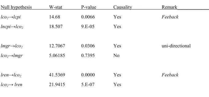
Series of additional diagnostic and robustness test was conducted for the current study. Prior to
the diagnostic test, the panel Granger causality by Dumitrescu and Hurlin (2012) as revealed in
Table 4 shows that past historical information of renewable energy consumption is a good at
explaining carbon dioxide emissions and with feedback. The same significant evidence is
observed between the consumer price index and the carbon dioxide emissions, also with
feedback. Expectedly, migration is observed to Granger cause the emissions of carbon dioxide
but without feedback.
An interesting part of this study is the result of the robustness check. The robustness check is
conducted by replacing the CO2 in the model (equation 1) with the GHG. The result (see Table
3) presents a complete replica of the first model, such that the direction of impact of all the
examined factors (variables) are the same. For instance, while renewable energy consumption
and consumer price index are negatively related with the CO2 emissions the impacts of GDP and
migration on CO2 emissions are positive. Also, the magnitude of the coefficient of estimations in
the two cases (model with CO2 and GHG) are of very small differential values.
The Wald test was observed to be significant in the two scenarios as indicated in the lower part
of Table 3. Additionally, the residual diagnostic tests (see Table 4) show that there is no concern
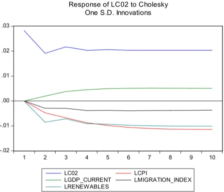
serial correlation’ and homoscedasticity at the statistical level of 1%. Lastly, the response of CO2
emissions to Cholesky one standard deviation (in this case 1% shocks in the independent
variables) is significant as indicated in Figures 1 and 2.
5. Concluding remarks
It is important to note that France, Germany, and the United Kingdom are uniquely related in few
numbers of ways, that include the economies, energy trend, climatic composition, migration
trend, and among others. As such, the present study investigated the dilemma associated with the
effects of renewable energy consumption and migration trend on the carbon dioxide emissions in
the panel countries over the period of 1990 to 2016. Sharing the mandate of an improved
environmental degradation caused by greenhouse gas (such as CO2), the countries have
consistently reassured their commitment toward a sustainable and more efficient energy
portfolio. Importantly, in our study, renewable energy consumption is observed to cause 0.13%
and 0.14% decline in the emissions of carbon dioxide with FMOLS and DOLS respectively.
Similarly, the study observed that migration causes 0.04% and 0.05% increase in the emissions
of carbon dioxide in the panel countries with FMOLS and DOLS respectively. Desirably, the
declining effect of renewable energy consumption on the carbon dioxide emissions is way higher
than the counter impact of migration on the carbon dioxide emission. In spite of the aforesaid
desirable observation, the panel countries would still have to strategically pursue the individual
country policies on renewable energy and carbon dioxide emissions with keen and sustainable
efforts.
In practical term, the EU member countries have an existing mandate on binding national targets
to raise the shares of renewables in the energy consumption by 20% by the year 2020. Since
is expected that the countries further explore its renewable energy resources, like rivers suitable
for hydroelectric power, effective utilization of sunshine for energy generation. Hence, the policy
of the government should be geared toward encouraging the stakeholders, especially private
investors and households to adopt more renewable energy portfolios. Because transportation and
industrial sectors are known to account for the larger proportion of carbon dioxide emissions in
the EU countries, the union’s target of attaining 15% and 30% reduction in average emissions of
continent’s fleet of new cars by 2025 and 2030 respectively should be further prioritized. The
investment policies of the government of the examined countries, especially which is tailored
toward renewable energy should cover more sectors of the economy. For example, France which
was originally observed to consume more renewables have been overtaken by Germany while
the UK continues to struggle in the development of renewables mostly because of investment
policies.
Except for Germany, the United Kingdom and France have in recent time exercise cold feet in
their response toward easing migrants and refugees’ movement. Since the study observed that a
more tolerable migrant atmosphere in the countries will cause more environmental degradation
(more CO2 emissions), it suggests that the countries implement their migration policies
painstakingly as to avoid disservice of their sustainable energy efficient and cleaner
energy/economy strategies. In future time, other empirical approach that captures the destination
and origin countries of the migrants could be studied in a comparative analysis.
References
Ahmadalipour, A., Moradkhani, H., Castelletti, A., & Magliocca, N. (2019). Future drought risk
in Africa: Integrating vulnerability, climate change, and population growth. Science of
Akadiri, S. S., Alola, A. A & Akadiri, A. C., & Alola, U. V. (Forthcoming). Renewable energy
consumption in EU-28 countries: Policy toward pollution mitigation and economic
sustainability. Energy Policy.
Al-mulali, U., Sab, C. N. B. C., & Fereidouni, H. G. (2012). Exploring the bi-directional
long-run relationship between urbanization, energy consumption, and carbon dioxide
emission. Energy, 46(1), 156-167. doi.org/10.1016/j.energy.2012.08.043.
Al-Mulali, U., Tang, C. F., & Ozturk, I. (2015). Does financial development reduce
environmental degradation? Evidence from a panel study of 129
countries. Environmental Science and Pollution Research, 22(19), 14891-14900.
doi.org/10.1007/s11356-015-4726-x.
Alola, A. A., & Alola, U. V. (2018a). The Dynamics of Tourism—Refugeeism on House Prices
in Cyprus and Malta. Journal of International Migration and Integration, 1-16.
Alola, A. A., & Alola, U. V. (2018b). Agricultural land usage and tourism impact on renewable
energy consumption among Coastline Mediterranean Countries. Energy & Environment,
0958305X18779577.
Alola, A. A. (2019). The trilemma of trade, monetary and immigration policies in the United
States: Accounting for environmental sustainability. Science of The Total
Environment, 658, 260-267.
Apergis, N., Jebli, M. B., & Youssef, S. B. (2018). Does renewable energy consumption and
health expenditures decrease carbon dioxide emissions? Evidence for sub-Saharan Africa
Atinkpahoun, C. N., Le, N. D., Pontvianne, S., Poirot, H., Leclerc, J. P., Pons, M. N., & Soclo,
H. H. (2018). Population mobility and urban wastewater dynamics. Science of the Total
Environment, 622, 1431-1437.
Aunan, K., & Wang, S. (2014). Internal migration and urbanization in China: Impacts on
population exposure to household air pollution (2000–2010). Science of the Total
Environment, 481, 186-195.
Baiocchi, G., Minx, J., & Hubacek, K. (2010). The impact of social factors and consumer
behavior on carbon dioxide emissions in the United Kingdom: A regression based on
input− output and geodemographic consumer segmentation data. Journal of Industrial
Ecology, 14(1), 50-72. doi.org/10.1111/j.1530-9290.2009.00216.x.
Bekun, F. V., Alola, A. A., & Sarkodie, S. A. (2019). Toward a sustainable environment: Nexus
between CO2 emissions, resource rent, renewable and nonrenewable energy in 16-EU
countries. Science of The Total Environment, 657, 1023-1029.
British Petroleum (BP, 2018). BP Statistical Review of World Energy.
https://www.bp.com/en/global/corporate/energy-economics/statistical-review-of-world-energy/downloads.html. (Accessed 1st September 2018).
Cansino, J. M., Román, R., & Ordonez, M. (2016). Main drivers of changes in CO2 emissions in
the Spanish economy: A structural decomposition analysis. Energy Policy, 89, 150-159.
doi.org/10.1016/j.enpol.2015.11.020.
Cooper, J., Stamford, L., & Azapagic, A. (2018). Sustainability of UK shale gas in comparison
with other electricity options: Current situation and future scenarios. Science of the Total
Dong, K., Jiang, H., Sun, R., & Dong, X. (2018). Driving forces and mitigation potential of
global CO2 emissions from 1980 through 2030: Evidence from countries with different
income levels. Science of the Total Environment. doi.org/10.1016/j.scitotenv.2018.08.326
Duman, Y. S., & Kasman, A. (2018). Environmental technical efficiency in EU member and
candidate countries: A parametric hyperbolic distance function approach. Energy, 147,
297-307. doi.org/10.1016/j.energy.2018.01.037.
Dumitrescu E I and Hurlin C (2012) Testing for Granger non-causality in heterogeneous
panels. Economic Modelling, 29(4), pp.1450-1460.
doi.org/10.1016/j.econmod.2012.02.014.
Farhani, S., & Ozturk, I. (2015). The causal relationship between CO 2 emissions, real GDP,
energy consumption, financial development, trade openness, and urbanization in
Tunisia. Environmental Science and Pollution Research, 22(20), 15663-15676.
doi.org/10.1007/s11356-015-4767-1.
Fernández-Sastre, J., & Montalvo-Quizhpi, F. (2019). The effect of developing countries'
innovation policies on firms' decisions to invest in R&D. Technological Forecasting and
Social Change.
European Union Commission (EU, 2018). EU Commission, DG ENER, Unit A4. Energy
Statistics. (Accessed 09/09/2018).
Economic Policy Uncertainty (EPU, 2018).
http://www.policyuncertainty.com/categorical_epu.html. (Accessed 01/09/2018).
Grossman, G. M., & Krueger, A. B. (1995). Economic growth and the environment. The
Han, L., Zhou, W., Li, W., & Qian, Y. (2018). Urbanization strategy and environmental changes:
An insight with relationship between population change and fine particulate
pollution. Science of the total environment, 642, 789-799.
Im, K. S., Pesaran, M. H., & Shin, Y. (2003). Testing for unit roots in heterogeneous panels.
Journal of econometrics, 115(1), 53-74. doi.org/10.1016/S0304-4076(03)00092-7. Intergovernmental Panel on Climate Change (IPCC, 2014). http://www.ipcc.ch/report/ar5/syr/.
(Accessed 2/09/2018).
International Renewable Energy Agency (IRENA, 2018). Renewable Capacity Statistics 2018.
http://www.irena.org/. (Accessed 2/09/2018).
Karmellos, M., Kopidou, D., & Diakoulaki, D. (2016). A decomposition analysis of the driving
factors of CO2 (Carbon dioxide) emissions from the power sector in the European Union
countries. Energy, 94, 680-692. doi.org/10.1016/j.energy.2015.10.145.
Kao, C. (1999). Spurious regression and residual-based tests for cointegration in panel
data. Journal of econometrics, 90(1), 1-44. doi.org/10.1016/S0304-4076(98)00023-2.
Kasman, A., & Duman, Y. S. (2015). CO2 emissions, economic growth, energy consumption,
trade and urbanization in new EU member and candidate countries: a panel data
analysis. Economic Modelling, 44, 97-103. doi.org/10.1016/j.econmod.2014.10.022.
Levin, A., Lin, C. F., & Chu, C. S. J. (2002). Unit root tests in panel data: asymptotic and
finite-sample properties. Journal of econometrics, 108(1), 1-24.
doi.org/10.1016/S0304-4076(01)00098-7.
Long, X., Naminse, E. Y., Du, J., & Zhuang, J. (2015). Nonrenewable energy, renewable energy,
carbon dioxide emissions and economic growth in China from 1952 to 2012. Renewable
Lu, I. J., Lin, S. J., & Lewis, C. (2007). Decomposition and decoupling effects of carbon dioxide
emission from highway transportation in Taiwan, Germany, Japan and South
Korea. Energy policy, 35(6), 3226-3235. doi.org/10.1016/j.enpol.2006.11.003.
Ma, G., & Hofmann, E. T. (2018). Immigration and environment in the US: A spatial study of air
quality. The Social Science Journal.
Maddala, G. S., & Wu, S. (1999). A comparative study of unit root tests with panel data and a
new simple test. Oxford Bulletin of Economics and statistics, 61(S1), 631-652.
doi.org/10.1111/1468-0084.0610s1631.
Moutinho, V., Madaleno, M., & Silva, P. M. (2016). Which factors drive CO2 emissions in
EU-15? Decomposition and innovative accounting. Energy Efficiency, 9(5), 1087-1113.
doi.org/10.1007/s12053-015-9411-x.
Nguyen, K. H., & Kakinaka, M. (2018). Renewable energy consumption, carbon emissions, and
development stages: Some evidence from panel cointegration analysis. Renewable
Energy. doi.org/10.1016/j.renene.2018.08.069.
Phillips, P. C., & Hansen, B. E. (1990). Statistical inference in instrumental variables regression
with I (1) processes. The Review of Economic Studies, 57(1), 99-125.
doi.org/10.2307/2297545.
Rafiq, S., Nielsen, I., & Smyth, R. (2017). Effect of internal migration on the environment in
China. Energy Economics, 64, 31-44.
Robaina-Alves, M., Moutinho, V., & Costa, R. (2016). Change in energy-related CO2 (carbon
dioxide) emissions in Portuguese tourism: a decomposition analysis from 2000 to
2008. Journal of Cleaner Production, 111, 520-528.
Saikkonen, P. (1992). Estimation and testing of cointegrated systems by an autoregressive
approximation. Econometric theory, 8(1), 1-27. doi.org/10.1017/S0266466600010720.
Shuai, C., Chen, X., Wu, Y., Zhang, Y., & Tan, Y. (2019). A three-step strategy for decoupling
economic growth from carbon emission: Empirical evidences from 133
countries. Science of the Total Environment, 646, 524-543.
doi.org/10.1016/j.scitotenv.2018.07.045.
Sówka, I., & Bezyk, Y. (2018). Greenhouse gas emission accounting at urban level: A case study
of the city of Wroclaw (Poland). Atmospheric Pollution Research, 9(2), 289-298.
Soytas, U., & Sari, R. (2009). Energy consumption, economic growth, and carbon emissions:
challenges faced by an EU candidate member. Ecological economics, 68(6), 1667-1675.
doi.org/10.1016/j.ecolecon.2007.06.014.
Stock, J. H., & Watson, M. W. (1993). A simple estimator of cointegrating vectors in higher
order integrated systems. Econometrica: Journal of the Econometric Society, 783-820.
DOI: 10.2307/2951763.
UNFCC, C. (2015). Paris agreement. FCCCC/CP/2015/L. 9/Rev.1. (Accessed 2nd September
2018).
United Nations Environment Program (UNEP, 2018). Global trends in renewable energy
investment 2018.
https://fs-unep-centre.org/publications/global-trends-renewable-energy-investment-report-2018. (Accessed 09/09/2018).
Wang, Y., & Zhao, T. (2018). Impacts of urbanization-related factors on CO2 emissions:
Evidence from China's three regions with varied urbanization levels. Atmospheric
World Development Indicator (WDI, 2018). World Bank database.
https://data.worldbank.org/products/wdi. (Accessed 09/09/2018).
Yu, Y., Deng, Y. R., & Chen, F. F. (2018). Impact of population aging and industrial structure on
CO2 emissions and emissions trend prediction in China. Atmospheric Pollution
Figure 1: Response of lco2 to the joint dynamics of the dependent variables -.02 -.01 .00 .01 .02 .03 1 2 3 4 5 6 7 8 9 10 Response of LC02 to LC02 -.02 -.01 .00 .01 .02 .03 1 2 3 4 5 6 7 8 9 10 Response of LC02 to LCPI -.02 -.01 .00 .01 .02 .03 1 2 3 4 5 6 7 8 9 10 Response of LC02 to LGDP_CURRENT -.02 -.01 .00 .01 .02 .03 1 2 3 4 5 6 7 8 9 10 Response of LC02 to LMIGRATION_INDEX -.02 -.01 .00 .01 .02 .03 1 2 3 4 5 6 7 8 9 10 Response of LC02 to LRENEWABLES
Figure 2: Response to Cholesky one S.D Innovations of the independent variable by lco2.
-.02 -.01 .00 .01 .02 .03 1 2 3 4 5 6 7 8 9 10 LC02 LCPI LGDP_CURRENT LMIGRATION_INDEX LRENEWABLES Response of LC02 to Cholesky One S.D. Innovations
Table 1: Descriptive statistics of the variables__________________________________________________________________________________
C Var. Mean Median Min. Max. S.D Skewness Kurtosis Jarque-Bera___
France co2 409.1400 415.5556 350.2279 439.8866 26.50921 -0.873781 2.679274 3.551442 ghg 542.9861 555.0549 470.6736 581.9684 33.98103 -0.965687 2.596895 4.379288 cpi 89.94863 89.25285 71.18813 105.7726 11.06784 0.016828 1.705049 1.887784 gdp 1640.844 1637.438 1004.342 2228.857 399.9351 -0.093218 1.604530 2.229857 mgr 95.96600 94.26027 31.16654 210.6428 39.75226 0.929742 2.062754 3.887730 ren 10.13922 9.821000 8.347000 12.36600 1.103988 0.382269 2.123725 1.521425 Germany co2 909.4565 914.8755 814.3457 1064.957 64.69484 0.371279 2.673436 0.740292 ghg 1052.392 1054.422 927.2303 1263.708 94.71261 0.391400 2.240141 1.338934 cpi 90.24528 89.55746 67.47511 107.4173 11.63153 -0.147878 2.052276 1.108859 gdp 2276.938 2220.080 1506.671 3144.050 448.4764 0.135985 2.263987 0.692643 mgr 144.4388 114.6983 25.29562 359.9762 100.8772 0.803310 2.478664 3.209646 ren 7.622778 6.968000 2.670000 14.27000 4.236774 0.184744 1.428424 2.932168 United Kingdom co2 565.3703 589.2337 428.9248 621.7030 53.25304 -1.242670 3.327753 7.069877** ghg 706.3776 733.3776 516.8034 821.0381 87.07855 -0.738075 2.389528 2.870654 cpi 87.76867 84.44838 62.43012 112.5419 14.77592 0.312958 2.023479 1.513532 gdp 1701.563 1811.401 936.3691 2602.156 491.2612 -0.229664 1.945480 1.488370 mgr 38.9754 2 6.35143 2 2.47347 105.9343 20.69683 1.6608.11 5.547176 19.71189* ren 1.437593 0.824000 0.398000 4.099000 1.209322 0.976303 2.394088 4.702278
Note: The series for both Cyprus and Malta are normally distributed. Min, Max, S.D implies Minimum, Maximum and Standard Deviation respectively. Co2,
ghg, cpi, gdp, mgr and ren are carbon dioxide emissions, greenhouse gas, consumer price index, real gross domestic product, migration index, and renewables respectively. Gdp is measured in Mrd (billion) Euro current prices, Co2 and ghg are measured in Mio tons and ren is measured in Mtoe.
Table 2: Panel unit root test_______________________________________________________________________________________________ LLC IPS Fisher-ADF Variable c t c t c t ______ lco2 1.54010 0.75426 2.46398 0.86744 2.90174 11.9541 lghg 1.83754 1.38625 3.36952 1.25171 1.87894 9.49365 lcpi 3.52490* -0.61838 -1.81407** -1.39468 19.2999* 14.4853** lgdp -2.92347* 1.00593 -0.19876 1.57542 6.73203 2.79701 lmgr -4.71800* -4.68887* -4.24203* -3.61192* 28.3948* 22.4048* lren 0.42429 -0.68497 1.47471 0.13689 1.67396 4.00703 ∆lco2 -7.24323* -7.64429* -7.19336* -8.66690* 51.0684* 56.6783* ∆lghg -6.95013* -5.95189* -7.11179* -8.06774* 50.7029* 54.1631* ∆lcpi -2.54812* -1.35995*** -2.34870* -1.28495*** 17.3581* 12.9447** ∆lgdp -5.61754* -5.52420* -4.39977* -2.01128* 29.0836* 24.8416* ∆lmgr -8.09246* -4.42464* -9.57601* -8.88245* 66.9015* 58.8114* ∆lren -5.96247* -3.55987* -6.11748* -4.26132* 41.5397* 26.9221* _____________________________________________________________________________________________________________________ Cross-sectional dependence test
Test lco2 lghg lcpi lgdp lmgr lren
Breusch-Pagan LM 49.94137* 60.92486* 79.36126* 71.97737* 8.40368 28.94004*
Breusch-Pagan LM 17.93899* 22.42298* 29.94961* 26.93515* 0.981297 9.365231*
Pesaran CD 6.976929 7.770899* 8.908475* 8.480003* 2.768594 4.973043
_____________________________________________________________________________________________________________________ Note: * and ** are statistical significance at 1% and 5% respectively. ∆ indicates first difference. Lag selection by SIC of maximum of 4 in all estimations.
LLC, IPS and Fisher-ADF are the Levin, Lin and Chu (2002); Im, Pesaran and Shin (2003); Fisher-ADF by Maddala & Wu (1999) panel unit root tests. For the Cross-sectional dependence test, ( ) is the p-value. C and t are the intercept and trend respectively and L implies the logarithmic transformation.
Table 3: Cointegration and long-run cointegration estimations___________________________________
Pedroni Residual Panel Cointegration
Panel Weighted panel Grouped
V-statistic 1.5(0.06) v-statistic 1.14(0.13) rho-statistic -1.4(0.08) Rho-statistic -1.87(0.03)** rho-statistic -1.76(0.03)** PP-statistic -5.0(0.00)* PP-statistic -4.53(0.00)* PP-statistic -4.41(0.00)* rho-statistic -5.5(0.00)* ADF-statistic -4.18(0.00)* ADF-statistic -3.99(0.00)*
Kao Residual cointegration
ADF {t-statistic} (p-value) {-5.126742} (0.0000*
FMOLS and DOLS long-run cointegration estimates
FMOLS DOLS With ghg G P P-W G P P-W lcpi -0.58* -0.41 -0.95* -0.43 -0.28 -0.95* lgdp 0.12 0.08 0.90* 0.13 -0.02 0.90* lmgr 0.03* 0.03** 0.12** 0.06* 0.005 0.12** lren -0.12* -0.06 0.31* -0.14** -0.08* 0.31* With co2 lcpi -0.66** -0.01 -1.30* -0.42 -0.30 -0.35 lgdp 0.25** 0.10 1.34* 0.23 0.09 0.11 lmgr 0.04* 0.06** 0.07 0.05* 0.01 0.01 lren -0.13* -0.07 0.45* -0.14** -0.06** -0.06
Wald Test, H0: Coefficients of larr and lmgr = lren = 1 (consider the Grouped estimations only)
lco2 lghg
Grouped FMOLS: t-Stat = 10400*, χ2 Stat =20801* t-Stat = 13653*, χ2 Stat =27306* Grouped DOLS: t-Stat = 2435*, χ2 Stat =4870* t-Stat = 2974*, χ2 Stat =5949*
_____________________________________________________________________________________
Note: The lag selection by Schwarz Information Criteria (SIC) due to the number (small) of observations. FMOLS
and DOLS are the Fully-modified ordinary least square and dynamic ordinary least square long-run estimation approaches. * and ** are respectively the 1% and 5% statistical significance level. Also, G, P and P-W are estimates for Group, Pooled and Pooled Weighted respectively.
Table 4: Diagnostic tests and Panel Granger causality__________________________________________
Residual Serial Correlation LM Test
LM-stat = 23.81561 (p-value = 0.5300)
Residual Heteroskedasticity Test
Chi-square = 212.2452 (p-value = 0.0503)
Dumitrescu and Hurlin (2012) test
Null hypothesis W-stat P-value Causality Remark_____________
lco2→lcpi 14.68 0.0066 Yes Feeback
lncpi→lco2 18.507 9.E-05 Yes
lmgr→lco2 12.7067 0.0306 Yes uni-directional
lco2→lmgr 5.06185 0.7395 No
lren→lco2 41.5369 0.0000 Yes Feeback
lco2→ lren 21.9415 5.E-07 Yes
Note: Co2, ghg, cpi, gdp, mgr and ren are carbon dioxide emissions, greenhouse gas, consumer price index, real gross domestic product, migration index, and renewables respectively. P-value is the probability value.