DESIGN OF LOW-PASS LADDER NETWORKS WITH MIXED LUMPED AND DISTRIBUTED ELEMENTS BY MEANS OF ARTIFICIAL NEURAL NETWORKS

NUMBER : 2

Received Date : 05.01.2003

DESIGN OF LOW-PASS LADDER NETWORKS WITH MIXED

LUMPED AND DISTRIBUTED ELEMENTS BY MEANS OF

ARTIFICIAL NEURAL NETWORKS

Metin ŞENGÜL

1

Atilla ÖZMEN

2

Melek YILMAZ

3

Kadir Has University, Engineering Faculty, 34230 Cibali, Fatih, İstanbul Tel: +90 212 534 10 34

1 _{E-mail: msengul@khas.edu.tr} 2_{E-mail: aozmen@khas.edu.tr} 3_{E-mail: myilmaz@khas.edu.tr}

ABSTRACT

In this paper, calculation of parameters of low-pass ladder networks with mixed lumped and distributed elements by means of artificial neural networks is given. The results of ANN are compared with the values that are desired. It has been observed that the calculated and the desired values are extremely close to each other. So this algorith can be used to obtain the parameters that will be used to synthesize such circuits.

Keywords: Lumped and distributed elements, artificial neural networks, back propagation

I. INTRODUCTION

One of the fundamental problems in the design and development of communication systems is to match a given device to the system via coupling circuits so as to achieve optimum performance over the broadest possible frequency band. This problem inherently involves the design of an equalizer network to match the given complex impedances, and usually referred as impedance

matching or equalization.

It has been appreciated for quite long time that networks containing both lumped and distributed elements offer many agvantageous associated with the present day emphasis on integrated circuits and more suitable especially for microwave filter applications, than those containing only lumped or distributed elements. The design of mixed lumped-distributed structures has been studied by several authors, by using as well as practical design techniques [1] and also by multivariable network synthesis techniques [1]. The problem has gained renew interest because of the possible application of the

mixed element structures as the reference networks for the design of multidimensional Wave Digital Filters [1].

In the second part of this paper, characterization of two-dimensional lossless two-ports by scattering approach will be given. The third part belongs to artificial neural networks. In the succeeding part, the calculation of the 5th _degrees

circuit (3 lumped and 2 distributed elements) parameters that will be used to synthesize the circuit and the obtained results can be found.

2. CHARACTERIZATION OF

DIMENSIONAL LOSSLESS

TWO-PORTS BY SCATTERING

APPROACH

In the theory of one-dimensional lossless two-ports, the so called scattering matrix and the corresponding scattering transfer matrix have turned out to be the most appropriate tools for establishing the synthesis theory. Of particular interest is the use of the Belevithc canonic forms of these matrices [1]. It is already known that, in the study of two-dimensional lossless two-ports, the scattering approach can be adopted as basis for the investigations.

Fettweis has shown that, the scattering matrix of a multidimensional reactance two-port with possible unit elements, as well as the corresponding scattering transfer matrix can be expressed in terms of canonic polynomials f, g and h [1]. In arriving at this description, the derivation follows essentially the same lines as in the one dimensional case, with the introduction of a particular type of multidimensional Hurwitz polynomials, namely Scattering Hurwitz or Principle Hurwitz polynomials, which plat yhe same role in multidimensional characterization as the classical Hurwitz polynomials so in one-dimensional case [1].

Before we consider the description of lossless two-ports by canonic polynomials, let us give first some basic definitions and the notation which will be used for the two-variable polynomials in the succeeding sections.

A polynomial g in two variables

p

,

λ

will be denoted by g(p,λ) or simply by g. g can be written as a polynomial in p and λ as

∑∑

= =

=

np k n l l k kl

p

g

p

g

1 1

)

,

(

λ

λ

λ

(1)

where and are the partial degrees of g in the variables p and λ respectively.

p

n

n

_λ

Definition 1: A two-variable polynomial g(p,λ) is said to be of degree m, if

)

(

max

₀

k

l

m

=

_gkl≠

+

p

n

_λ λ

n

n

m

_p

. In terms of the partial

degrees and

n

it is defines as

+

=

.

Arranging with respect to one of the variables with coefficient polynomials in the other variable, we obtain the recursive canonic form,

∑

∑

= − =

=

=

λ

λ

λ

λ

n l k n k k

_G

_p

p

G

p

g

p 1 1

)

(

)

(

)

,

(

(2)

Another form that we adopt for the representation of the two-variable polynomials is in matrix notation, T g T

p

p

g

(

,

λ

)

=

Λ

λ

(3) where

_p

T

[

_p

_p

_p

np

]

K

2

1

=

and

[

_K

λ

nλ

]

λ

xn

n

_p

λ

λ

λ

T

₌

₁

2 g and coefficient matrix

Λ

is defined by               = Λ λ λ λ n n n n n n g p p p g g g g g g g g g L M L M L L 1 0 1 11 10 0 01 00 (4)

The paraconjugate of the two-variable polynomials is defined as

g

_*

=

g

(

−

p

,

−

λ

)

.

Definition 2: A two-variable polynomial g(p,λ) is called as a mth-degree polynomial with no missing terms if it is expressible as

ij

∑ ∑

= − =













=

m k k k m l l kl

p

g

p

g

0 0

)

,

(

λ

λ

(5)

where are nonzero real constants. In matrix notation, this corresponds to the nonzro upper-triangular coefficient matrix form.

g

              = Λ 0 0 0 0 0 11 10 0 01 00 L L M L L p n n g g g g g g g _λ (6)

Now, let us consider two-variable characterization of lossless two-ports with mixed lumped-distributed elements and state the properties of canonic polynomials.

Consider the generic form of a lossless two-port formed with cascade connections of lumped and distributed two-ports as shown in Fig. 1.

Z1,ι Z2,ι

N1 N2 Nn

Figure 1 Generic form of cascaded lumped and distributed two-ports

The scattering matrix describing the mixed element two-port can be expressed in the Belevitch canonical form as [1],

      − − − − − = ) , ( ) , ( ) , ( ) , ( ) , ( 1 ) , ( λ σ λ λ σ λ λ λ p h p f p f p h p g p S (7) where

•

f

(

p

,

λ

)

is a monic real polynomial that consist of transmission zeros,

•

h

(

p

,

λ

)

ve

g

(

p

,

λ

)

are real

polynomials in the complex variables

jw

p

=

σ

+

and

λ

=

ε

+

j

Ω

(

λ

=

tanh( p

τ

),

τ

being the delay length of unit elements),

)

,

(

p

λ

g

σ

, ( ) , ( ) ,−λ = λ − −p h p h p β µ α µ ) 2 2 , / , ( ) 2 ) 1 ) 2 2 30 01 20 11 20 11 2 / 1 30 10 30 10 2 20 10 21 21 12 30 30 30 12 2 / 1 20 2 10 11 2 / 1 2 02 11 2 / 1 2 01 02 g g h h g g h h g g h g g h g g g h h g g h h h h g g h g + − − − + = = = = = + = + = + + • is a Scattering Hurwitz polynomial, • is a unimodular constant;

σ

=

1

, • Losslessness of the mixed element

two-port requires that

) , ( ) , ( ) ( ) , (p λ g −λ + f p λ f −p−λ g .

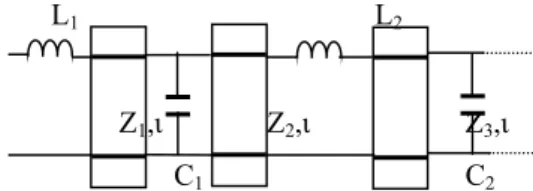
From the physical implementation point of view, one practical circuit configuration is that of simple low-pass ladder sections connected with unit elements (LPLUE) as shown in Fig. 2.

L1 L2

Z1,ι Z2,ι Z3,ι

C1 C2

Figure 2 Low-pass ladder with unit element In the Table 1, the explicit formulas for 5th order LPLUE are given.

n Coefficient Relations 5 [h01,h02,h10,h20,h30] independent coefficients β µ µ µ α β α α β / ) ( ( / ) ( / / ( ( 30 01 21 20 10 12 01 01 30 02 11 02 11 10 20 02 02 01 10 01 10 01 h h g g h h h g h h g g g h g h h g g = = − = − = − = + = − =

3. NEURAL NETWORKS

Artificial neural networks (ANN) which consist of simplified neurons connected to each other are the models of nervous system. Although each neuron has a simple function alone, they can be used to solve complex problems, when they are used together.

Artificial neural networks are adaptive systems which have learning capabilities. ANNs adapt and organize themselves to the changing conditions, improve a function and make the calculation by learning. ANNs can produce the correct response even though missing or corrupted input is given to them. They are more suitable for the daily life problems because of their nonlinear characteristics [2].

In Figure 3, a neuron can be seen which consists of a summing junction and a non-linear activation function. Here, x1, x2, …,xn are inputs;

w1, w2,…, wn are synaptic weight coefficients

and y is output.

in in

Figure 3 Neuron model

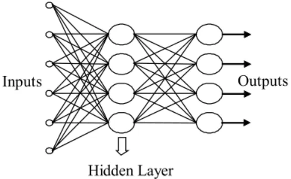
A neural network model can be seen in Figure 4. Each neuron has many inputs and only one output, and this output is the input for the other neurons, so system is formed in parallelly.

Inp uts Outputs

Hidden Layer

Figure 4 ANN with one hidden layer

ANNs can be used in signal processing, image processing, pattern recognition, medical, military systems, finance systems, artificial intelligence and power systems.

3.1. Learning in Artificial Neural

Networks

Learning in artificial neural networks is based on the calculation of the synaptic weight coefficients suitable for the problem. Learning rule is an equation set by which all or some of the synaptic weight coefficients change so as to modify the response of each neuron in time. By this way ANN can adapt itself to get the desired response.

ANNs are learnt by example data instead of programming. Learning process can be divided into two groups; supervised and unsupervised learning.

In supervised learning, both the input and the response are given to the system. For each input, obtained response and desired response are compared. To get the minimum difference, synaptic weight coefficients are changed. When an acceptable error is obtained, learning process is stopped and then these synaptic weight coefficients can be used with the data that are not used in learning process.

Σ

x1 x2 x3 xn b w1 w2 w3 wn u=w 0 x 0 +w 1 x1+ w 2 x 2 +...+w n x n put bias output y weight

coefficients non-linear function

Σ

x1 x2 x3 xn b w1 w2 w3 wn u=w 0 x 0 +w 1 x1+ w 2 x 2 +...+w n x n put bias output y weight

coefficients non-linear function

y=f(u+b) y=f(u+b)

3.2. Back Propagation Algorithm

In this paper, back propagation algorithm is used as the learning algorithm, which has emerged as the most widely used and successful algorithm for the design of multiplayer feedforward networks [3].

In learning process, first of all, an error is obtained by subtracting the result from the desired value. Then the error is squared. In this algorithm, it is desired to realize a learning process with an error whose square is minimum.

2 2

₌

₍

_t

₋

_y

₎

ε

(8)

)))

(

(

(

y

u

w

ε

ε

=

(9)

Then delta values are calculated at the output nodes.

w

w

_∂

∂

≡

∇

_ε

2

ε

2 ₍₁₀₎

And by using back propagation, all the values at the output nodes are calculated.

x

x

u

sgm

w

u

u

y

y

w

δ

ε

ε

ε

2

)

(

2

' 2 2

=

−

=

∂

∂

⋅

∂

∂

⋅

∂

∂

=

∇

(11)

)

x

(

'

_u

sgm

ε

δ

≡

−

(12)

Finally, the components of gradient are calculated and desired synaptic weight coefficients are obtained.

w

=

−

2

µ

δ

∆

(13)

w

     

w

w

_new

=

_old

+

∆

(14)

4. EXAMPLE AND CONCLUSION

In this section, we solve the classical double matching problem. Here, an LPLUE network of degree five, (np=3, nλ=3) will be constructed over the normalized frequency band of 0≤w≤1. In the course of the learning process, the coefficients

{h00,h01,h02,h10,h20,h30,g00,g01,g02,g10,g20, g30} are chosen as the input parameters, the other coefficients are derived by means of designed neural network.

We obtained the following coefficient matrices that completely describe the scattering parameters of the matching network under consideration. Also you can see the matrices that are derived via the explicit expressions given in Table 1. Ah=      − − − − − 0 0 9960 . 0 0 5316 . 3 1827 . 0 61081 . 1 3420 . 0 1042 . 0 6281 . 1 7310 . 1 0 Ag=             0 0 9960 . 0 0 5316 . 3 0746 . 2 6108 . 1 8760 . 5 0396 . 2 9107 . 1 9694 . 2 1 Ah=_ Ag=              − − − − − 0 0 9960 . 0 0 3089 . 2 1827 . 0 4744 . 5 6353 . 5 1042 . 0 6281 . 1 7310 . 1 0           0 0 9960 . 0 0 3454 . 6 0746 . 2 3960 . 4 7664 . 6 0396 . 2 9107 . 1 9694 . 2 1

h and g matrices derived by ANN and explicit expressions, respectivelly.

ZS C1 Z1 L Z2 C2 ZL

Fig 5. Double matching example with lumped-distributed elements [L=2.1439, C1=0.8825,

C2=1.0528, Z1=1.0356, Z2=3.6650, ι=0.2191],

[ZS=RS+jwLS, ZL=(RL//(1/jwCL)+jwLL)]

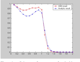
Fig 6. Gain performance of double matchingexample

5. REFERENCES

[1] Aksen, A., “Design of Lossloss

Two-ports with Mixed Lumped and Distributed Elements for Broadband Matching”, Doktora tezi, Ruhr Üniversitesi, Bochum, 1994

[2] HAYKIN, S., “Neural Networks”

Macmillan College Publishing Company Inc., 1994, ISBN: 0-02-352761-7

[3] Şengül.M, Özmen.A, Yılmaz.M, “Toplu

ve Dağınık Elemanlı Alçak-Geçiren Merdiven Tipi Devre Parametrelerinin Yapay Sinir Ağları Kullanılarak Hesaplanması”, Eleco 2002, Bursa