ON THE INVERSE POINT-SOURCE PROBLEM OF THE POISSON EQUATION
Tam metin
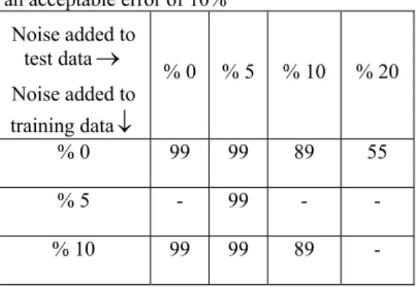
Şekil
Benzer Belgeler
Query by image content is the searching of images based on the common, intrin sic and high-level properties such as color, texture, shape of objects captured in the images and
3- Amin (2014) Analysis of geography for Problem of water pollution of the Sirwan River in the Kurdistan region, Environmental pollution investigation, The study area is
ANTIBACTERIAL ACTIVITY OF ROYAL JELLY AND RAPE HONEY AGAINST Aeromonas hydrophila (ATCC 7965) Deyan STRATEV 1 , Ivan VASHIN 1 , Ralitsa BALKANSKA 2 , Dinko DINKOV 1.. 1 Department
function edit5_Callback(hObject, eventdata, handles) function pushbutton2_Callback(hObject, eventdata, handles) data = getappdata(gcbf,
1898 yılında kurmay yüzbaşı olarak akademiyi bitirdikten sonra Arnavutluk’ ta görev yapmış, Arnavutluk ve Rumeli vilayetleriyle ilgili ıslahat kararla rını uygulamakla
Upon IRF3 phosphorylation, Type I IFN genes are up-regulated and innate immune cells such as macrophages, dendritic cells and monocytes abundantly secrete
Our goal is to design an isolation network that improves the bandwidth of input return loss, output return loss and isola- tion, simultaneously.. This way, the number of sections is
Therefore all these factors were observed and photos were taken in this study carried out in the Kanuni campus of Karadeniz Technical University.. The obtained materials
