F Ö !? £ C ^ S T !H G Т Щ F Q » £ i S ä
G ü S S E H C Y P R I S E S t iS lla S
g ШШ і Ш Ш
8
à P P s S â â S i
i“ ί Гл ! |j 11J »i *5i» w4 1? W ж ^ .üt
1·()ΚΚΓΛ8ΐ1Ν<; THK FÜliKKiN CIİRKKNCV H R K 'K S IJSIN(; ΓΙΙΕ BOX JE N K IN S APPROACH
A THESIS
SUBMITTED TO THE DEPARTMENT OF MANAGEMENT AND THE GRADUATE SCHOOL OF BUSINESS ADMINISTRATION
OF BILKENT UNIVERSITY
IN PARTIAL FULFILLMENT OF THE REQUIREMENTS FOR THE DEGREE OF
MASTER OF BUSINESS ADMINISTRATION
By
BELGİN İNAN June, I9B‘J
f I О ^
K G -г»
in i
H TSCf® і е б
5
I certify that I have read this thesis and that in my opinion it
is fully adequate, in scope and quality, as a thesis for the
degree of Master of Business Administration.
Assist. Prof. Dilek Yeldan
I certify that I have read this thesis and that in my opinion it
is fully adequate, in scope and quality, as a thesis for the
degree of Master of Business Administration.
Assist. Prof. Kürsat AydoQan
I certify that I have read this thesis and that in my opinion it
is fully adequate, in scope and quality, as a thesis for the
degree of Master of Business Administration.
Assist. Prof. Erdal Erel
Approved for the Graduate School of Business Administration
Prof. Dr. Subidey Togan
ACKNOWLEDGEMENT
I wish to thank Dr. Dilek Yeldan, Dr. Kursat AydoQan, and Dr.
Erdal Erel for their advice, guidance, and encouragement
throughout the course of this thesis.
ABSTRACT
FORECAST [NT. ΓΙΙΚ l-ORKiGN CURRENCY P R IC E S USING THE BOX JE N K I N S APPROACH
İnan M.B.A. in Management
Supervisor: Assist. Prof. Dilek Yeldan June 1989, 96 pages
In this thesis, the Box Jenkins approach is applied to forecast the future prices of foreign currencies, American Dollar and
German Mark, in Turkey’s Black Market using available
observations made between the years 1985-1988. The forecasts obtained from this approach are compared to the real available observations. The results show that the Box Jenkins approach is not accurate enough in this case because of the large mean absolute deviation between the forecasted and the observed values of these currencies due to the significant residuals generated in the diagnostic checking stage.
Ki-yworils; E’orecast:ing. Box Jenkins, foreign currency
OZIvT
BOX JKNKINS MKTÜDUNÜ KULLANARAK DÖVİZ FİYATLARININ TAHMİNİ
Belidin İnan
İs İdaresi Yüksek Lisans
Denetçi: Yrd. Doç. Dr. Dilek Yeldan Haziran 1989, 96 sayfa
Bu tezde Box Jenkins metodu ile Türkiye’de serbest piyasadaki Amerikan Doları’nın ve Alman Markı’nın değerleri, 1985-1988
yılları arasındaki gerçek değerler kullanılarak tahmin
edilmiştir. Elde edilen öngörüler gerçek değerlerle
karş1laştır1Imıştir. Teşhis kontrol aşamasında ortaya çıkan
anlamlı artıklara bağlı olarak, öngörülen sonuçlar ve gerçek sonuçlar arasındaki ortalama mutlak sapmaların büyüklüğü nedeni
ile, Box Jenkins metodunun verdiği sonuçların yeterli derecede doğru olmadığı gösterilmiştir.
CHAPTER 1- INTRODUCTION ... 1
1.1. Problem Definition ... 1
CHAPTER 2- FORECASTING METHODS ... 2
2.1. Introduction ... 2
2.2. Forecasting techniques 4 2.3. Box Jenkins method of forecasting ... 12
2.4. Common ARIMA processes ... 16
CHAPTER 3- APPLICATION OF BOX JENKINS METHOD USING AMERICAN DOLLAR ... 18
3.1. Identification ... 1*?
3.2. Estimation ... 21
3.3. Diagnostic checking ... 22
3.4. Forecasting ... 24
CHAPTER 4- APPLICATION OF BOX JENKINS METHOD USING GERMAN MARK ... 29
4.1. Identification ... 29
4.2. Estimation ... 30
4.3. Diagnostic checking ... 30
4.4. Forecasting ... 31
CHAPTER 5- RESULTS & CONCLUSIONS ... 35
REFERENCES ... 38 APPENDIX A- FIGURES ... 41 APPENDIX B- TABLES 78 TABLE OF CONTENTS Subject Page No V I
LIST OF FIGURES
Figure No Description Page No
3.1. The daily Dollar prices versus time in workdays 42
from September, 1985 till December, 1988
3.2. Estimated autocorrelation function for the 43
Dollar series
3.3. First differences of the Dollar values versus 44
time in workdays
3.4. Estimated autocorrelation function for the 45
first differenced Dollar series
3.5. Estimated partial autocorrelation function for 46
the first differenced Dollar series
3.6i Estimated residual autocorrelation function 47
for the Dollar series
3.7. Time sequence plot of residuals for Dollar 48
series for the years September, 1985 till
December, 1988
3.8. Time sequence plot of forecast function for 49
December, 1988 till March, 1989
3.9. Time sequence plot of real observations for 50
December, 1988 till March, 1989
LIST OF FIGURES CONTINUED
Figure No Description Page No
3.10 The daily Dollar prices versus time scale of 51
workdays from September, 1985 till March, 1989
3.11. First differences of the daily Dollar prices 52
of Figure 3.10
3.12. Estimated autocorrelation function for the 53
first differenced Dollar series
3.13. Estimated partial autocorrelations for the first 54
differenced Dollar series
3.14. Estimated residual autocorrelation function 55
for the Dollar series
3.15. Time sequence plot of the forecast function 56
for March and April, 1989
3.16. Time sequence plot of residuals for the years 57
September, 1985 till March, 1989
3.17. Time sequence plot of forecast function for the 58
second differenced Dollar series for March and April, 1989, model AR(2)
3.18. Time sequence plot of forecast function for 59
the first differenced Dollar series for March
and April, 1989, model AR(2), MA(1)
LIST OF FIGURES CONTINUED
Figure No Description Page No
4.1. The daily Mark prices versus time scale of 60
workdays from September, 1985 till December, 1988
4.2. Estimated autocorrelation function for the data 61
in Figure 4.1.
4.3. First differences of the Mark prices versus 62
time scale of workdays
4.4. Estimated autocorrelation function for the first 63
differenced Mark series
4.5. Estimated partial autocorrelation function for 64
the first differenced Mark series
4.6. Estimated residual autocorrelation function for 65
the Mark series
4.7. Time sequence plot of residuals from September, 66
1985 till December, 1988
4.0. Time sequence plot of forecast function from 67
December, 1988 till March, 1989
4.9. Time sequence plot of real observations from 68
December, 1988 till March, 1989
4.10. The daily prices versus time scale of workdays 69
LIST OF FIGURES CONTINUED
Figure No Description Page No
4.11. Estimated autocorrelation function for the
Mark series in Figure 4.10
4.12. First differences of the Mark series versus
time scale of workdays
4.13. Estimated autocorrelation function for the
first differenced Mark series
4.14. Estimated partial autocorrelation function
for first differenced Mark series
4.15. Estimated residual autocorrelation function
for the Mark series
4.16. Time sequence plot of residuals for the
Mark series
4.17. Time sequence plot of forecast function
including March and April, 1989
4.18. Time sequence plot of real observations
including March and April, 1989
70 71 72 73 74 75 76 77
LIST OF TABLES
Table No Description Page No
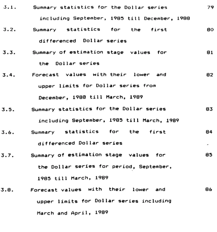
3.1. Summary statistics for the Dollar series 79
including September, 1985 till December, 1988
3.2. Summary statistics for the first 80
differenced Dollar series
3.3. Summary of estimation stage values for 81
the Dollar series
3.4. Forecast values with their lower and 82
upper limits for Dollar series from December, 1988 till March, 1989
3.5. Summary statistics for the Dollar series 83
including September, 1985 till March, 1989
3.6. Summary statistics for the first 84
differenced Dollar series
3.7. Summary of estimation stage values for 85
the Dollar series for period, September, 1985 till March, 1989
3.8. Forecast values with their lower and 86
upper limits for Dollar series including March and April* 1989
LIST OF TABLES CONTINUED
Table No Description Page No
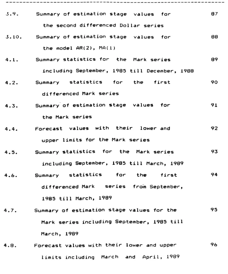
v5.9. Summary of estimation stage values for 87
the second differenced Dollar series
3.10. Summary of estimation stage values for 08
the model AR(2), MA(1)
4.1. Summary statistics for the Mark series 89
including September, 1985 till December, 1980
4.2. Summary statistics for the first 90
differenced Mark series
4.3. Summary of estimation stage values for 91
the Mark series
4.4. Forecast values with their lower and 92
upper limits for the Mark series
4.5. Summary statistics for the Mark series 93
including September, 1985 till March, 1989
4.6. Summary statistics for the first 94
differenced Mark series from September,
1985 till March, 1989
4.7. Summary of estimation stage values for the 95
Mark series including September, 1985 till March, 1909
4.0. Forecast values with their lower and upper 96
limits including March and April, 1989
CHAPTER 1
INTRODUCTION
1.1. P r o b l e m DefinitionRecent economic policies of C e ntral B ank in Turkey have had a
d r a s t i c impact on the Black Market pr i c es of foreign currencies and make s one wonder about the c h anges that are to occur in these
pric e s in the near future. Many news agencies have been ma king
s p e c u l a t i o n s about the future prices of foreign currencies based on the historical and current data.
Bef o r e A u g u s t 1988, Turkey's C e n t r a l B ank used to set the prices
of the foreign currencies w i thout taking into a ccount the
c o n d i t i o n s of the foreign exchange market in Turkey. This
p o l i c y produced a considerable d i f f e r e n c e between the prices
of the C e n t r a l Bank relative to the p r i c e s of the B l a c k Market. The fo reign exchange rates in the B l a c k Market turned out to be
chea p e r than the prices of the C e n t r a l Bank and for this
reason, m a n y investors and b u s i n e s s m e n preferred to b uy
foreign exchange from the Black M a r k e t rather than the C e n tral
Bank. As a result of this, the C e n t r a l Bank did v ery limited
b u s i n e s s related with foreign e x c h a n g e causing inefficient use
of the fo reign exchange market. S t a r t i n g August 1988, however,
the C e n t r a l B ank changed their p o l i c y by es tablishing new
d i v i s i o n s such as foreign excha n g e and effective exchange
mar k e t s in their body. This allowed the Central Bank to get a
b et t e r c o ntrol of the foreign e x c h a n g e prices in the Black
The Central Bank did not directly intervene the Black Market
in determining the prices of foreign currency, but rather
took some steps that affected these prices in the Black
Market. For example, the government made 57. devaluation in
1986, which resulted in an increase in the prices of foreign
currency in the Black Market, closing the gap between the prices
of foreign currency in the Black Market relative to the
Central Bank. This allows the government to make more
efficient use of foreign currency deposits of the Central Bank
in Turkey. In addition, another factor that could play
a key role for more efficient usage of foreign currency
deposits is to be able to forecast variations in these prices in
the future.
Because Turkey's outside loans are in the form of
Dollars, forecasting the prices of the foreign currency is
very important for Turkey. Some increase in the price of Dollar
can cause a large deficit of Turkey's Treasury and create major
economic problems. For this reason, forecasting the future
prices of foreign currency is important in controlling
the treasury of Turkish Government. Besides, foreign currency
prices affect the investors, especially those who are
importing foreign machines and raw material. By making proper
forecasting, they can control their budget more efficiently and
In this thesis, first, a brief summary on different forecasting
techniques is introduced in Chapter 2. This is followed by
the Box Jenkins method of forecasting that is applied to
project Turkey's Black Market prices of American
Dollar and German Mark for the period December, 1988 and January
and February, 1909 in Chapters 3 and 4. Then, same forecasts
are updated for the period March and April, 1989.
In Chapter 5, these forecast values obtained are then compared
with the real available data for the same time periods in terms
of mean absolute deviation of these two sets, namely the
forecasts and the observations. In addition, the accuracy of the
Box Jenkins approach is discussed based on the above comparisons and the accuracy of the available data.
CHAPTER 2 FORECASTING METHODS
2.1 Introduction
There is frequently a time lag between the realization that an
event is going to happen and the occurrence of that event. This
time lag is the main cause of planning and forecasting.
Forecasting is the act of making predictions of future events and
conditions. Forecasting is needed to determine if and when an
event is going to happen so that appropriate planning can be made to control the outcome of this event to a certain extent.
Planning can play an important role in management. Today, almost
every manager who is about to make a decision has to consider
some kind of forecast. Sound predictions of demands and trends
are no longer luxury items, but necessities for managers who need
to cope with seasonality, sudden changes in demand levels, price
cutting operations of the competition, strikes, and large swings
of the economy. Forecasting helps the manager in dealing with
these problems, and it helps best if the manager knows about the
general principles of forecasting, what it can and cannot do
currently, and which techniques are suitable to the needs at any
given time.
To handle the increasing variety and complexity of managerial
forecasting problems, many forecasting techniques have been
must be taken to select the most suitable technique for a
particular application. The manager as well as the forecaster
have roles to play in technique selection and the better
the manager understands the range of forecasting possibilities,
more likely it is that a company's forecasting efforts will
be successful.
The selection of a method depends on many factors. Some of these
factors are the context of the forecast, the relavence and
availibility of historical data, the degree of accuracy
desirable, the time period to be forecast, the cost/benefit (or
value) of the forecast to the company, and the time available for
making these analysis. Forecasting methods are discussed in the
There are two basic categories of forecasting techniques: 1. Qualitative techniques
2. Quantitative techniques
Qualitative techniques can be divided into two types of methods: 1-a. Exploratory methods
1. b. Normative methods
Quantitative techniques can also be divided into two types of methods.
2. a. Time series methods 2.b. Causal methods
1. Qualitative Methods
Qualitative methods use qualitative data such as expert
opinion. These methods are used when data are scare or when no
historical data are available. Qualitative methods can be divided into exploratory and normative methods.
2,2· Forecasting Techniques
l.a. Exploratory methods: start with today's knowledge and its
orientation and trends, and seek to predict what will happen in the future and when. An example is the Delphi Method. It involves circulating a series of questionnaires among individuals who have
the knowledge and ability to participate meaningfully. Responses
Each new questionnaire is developed using any information
extracted from the previous one, thus enlarging the scope of
information on which participants can base their judgements and to achieve a consensus forecast. However, the Delphi Method does
not require that a consensus be reached. Instead, it allows for
justified differences of opinion rather than attempting to
produce unanimity (Brown 1968).
l.b. Normative Methods: these methods begin with the future by
determining future goals and objectives, then work backwards to
see if these can be achieved, given the constraints, resources
and technologies available. An example is the relavence tree
approach. This method uses the ideas of the decision theory to assess the desirability of future goals and to select those areas
of technology whose development is necessary to the achievement
of those goals. The technologies can then be singled out for
further development by the appropriate allocation of resources (Wheelwright and Makridakis, 1980).
2. Quantitative Techniques
Quantitative techniques can be used when the following three
conditions are satisfied:
1. information about the past is available
2. this information can be quantified in the form of numerical
3. it can be assumed that some aspects of the past will continue in the future
Quantitative techniques can be divided into time series methods and causal
methods-2.a. Time Series Methods: a time series is a time-ordered
sequence of observations that have been taken at regular
intervals over a period of time (hourly, daily, weekly, monthly,
quarterly and so on). Analysis of time series data requires the
analyst to identify the underlying behavior of the series. These
behaviors can be described as follows:
♦ trends (gradual, long term movement in the data)
♦ seasonality (short-term, fairly regular, periodic variations) ♦ cycles (wave-like variations of more than one year's duration)
t irregular variations (due to unusual events)
♦ random variations are the residual variations that remain after
all of the other behaviors have been accounted for (William J.
Stevenson, 1986)
There are four approaches to the analysis of time series methods: 1. The naive approach.
2. Moving averages.
3. Exponential smoothing.
4. Decomposition of a time series.
accepted as the forecast for the next period. It works accurately if there is little variation in actual values in time series from period to period.
2. Moving averages: moving average is an average that is
repeatedly updated. As new observations added to the series, the
old observations are deleted from the series. In this way, the
average can be kept current. Moving averages can be simple or weighted moving averages. Simple moving average is the average value of a time series for a certain number of the most recent periods and accepting that average as the forecast for the next
period. Weighted moving average assigns weights to the
observations in a decreasing order from the recent observation to
the oldest one, then takes the average of these weighted
observations as the forecast for the next period.
3. Exponential smoothing: it is a form of weighted moving
average. The name exponential smoothing is derived from the way
weights are assigned to historical data, the most recent values
receive most of the weight and weights decrease exponentially as
the age of the data increases. The method is easy to use and
understand. Each new forecast is based on the previous forecast
plus a percentage of the difference between that forecast and the actual value of the series at that point. That is:
New forecast=01d forecast+ a (actual-old forecast)
This equation is the general form used in computing a forecast
with the method of exponential smoothing. Some of the smoothing
techniques used are as follows: 1. Brown's exponential smoothing
2. Holt's linear exponential smoothing 3. Winter's seasonal smoothing
1. Brown's exponential smoothing: Brown's method uses simple,
linear, or quadratic smoothing to generate forecasts for a time
series. Therefore Brown's method can be examined in three section as follows:
i. Brown's one-parameter adaptive method
ii. Brown's one-parameter linear method
iii. Brown's one-parameter quadratic method
Here, only the first method will be explained briefly·
i. Brown's one-parameter adaptive method: it involves a single
smoothing constant (with a value between 0 and 1), is very
general, and has given satisfactory performance in practical
situations· The equations used in this method are as follows:
Sts=Sti— i+bi"*·(1-r^
bt.=bt:-j. + ( l-r)2 .e^ e,:=Xt.-F.,
r = smoothing constant et=error term
b=trend adjustment
m=number of periods ahead to be forecast t=time
X=actual value F=forecast value
First equation, smooths the current values of the errors. This
approach is a different way of formulating the forecasts, which
can be combined with that of formulating the forecast based on
previous values of the series.
2. Holt's Linear Exponential Smoothing: this smoothing method is
similar in principal to Brown's method except that it does not
apply the straight forward double smoothing formula. Instead, it
smooths the trend values seperately. This provides greater
flexibility, since it allows the trend to be smoothed with a
different parameter than that used on the original series. Holt's
method uses two smoothing constants (with values 0 and 1) unlike
Brown who uses one smoothing constant for forecasting (for more
details see Wheelwright and Makridakis, 1983).
3. Winter's Seasonal Smoothing: It uses three smoothing constants
to generate forecasts for a seasonal time series. This method
involves three smoothing equations one for stationarity, one for
trend, and one for seasonality (for more details see Wheelwrigt and Makridakis, 1983).
The last approach to the analysis of time series methods is
the decomposition of time series.
4. Decomposition of Time Series: in this approach a time series
is viewed as being made up of four possible components: trend,
seasonality, cycles, and random plus irregular variations. This
approach aims to distinguish various components (except random and irregular variations) so their effects can be considered separately. In some situations, interest may focus on only one of these components instead of all of them. For example, a buyer for a department store may be more concerned with seasonal variations in demand than with long-term projections.
The second quantitative technique as mentioned at the beginning of the chapter is the causal methods.
2.b. Causal Methods: these methods assume that the factor to be
forecast shows a cause/effect relationship with a number of other
factors (for example, sales=f(income, prices, advertising,
competition, etc.)). The aim of the method is to discover that
relationship so that the future values of sales can be found using the values of income, price, advertising. Regression models
and multivariate time-series models are the most common
forecasting approaches of causal^ mode l s .
Although the methods discussed above may be suitable for short
term forecasting of time series, we can see cases where the real
life situation is much more complicated, and the pattern is made
up of combinations of a trend, a seasonal factor, and a cyclical
factor as well as the random f lue tuat i ons. In these cases a much
more comprehensive forecasting method is needed. The Box Jenkins
method of forecasting is particularly well suited to
handle this type of real situations (Wheeelwright and
Makridakis, 1980). In addition, forecasts from ARIMA models are
said to be optimal forecasts. This means that no other
univariate forecasts have a smaller mean squared forecast error. This technique is discussed next.
2-3 Box Jenkins Method of Forecasting
George E.P. Box and Gwilym M.Jenkins (Box,Jenkins 1976) are the
two researchers who have effectively put together in a
comprehensive manner the information required to understand and use univariate (single) time series ARIMA models. Univariate Box
Jenkins (UBJ) models are often referred to as ARIMA models. An
ARIMA (Autoregressive Integrated Moving Average) model is an
algebraic statement showing how observations on a variable are
statistically related to past observations on the same variable.
Autoregressive (AR) models are a form of regression, but instead
of dependent variable (the item to be forecast) being related to
independent variables, it is simply related to past values of
itself at varying time lags. Therefore AR models are those that
express the forecast as a function of previous values of that
time series. AR models are first introduced by Yule (1926) and
later generalized by Walker (1931).
MA (moving average) models in Box Jenkins modelling means that
the value of the time series at time t, is influenced by a
current error term and (possibly) weighted error terms in the
past. MA models were first used by Slutzky (1937). Later,
Wold (1938) provided the theoretical foundations of combined
ARMA (Autoregressive Moving Average) processes. In an ARMA
model, the series to be forecast is expressed as a function
of both previous values of the series (autoregressive terms) and previous error values (the moving average terms).
ARIMA models can be used if the following conditions exist in a time series: ARIMA are models suited to short term forecasting because most ARIMA models place heavy emphasis on the recent past
rather than the distant future. ARIMA models are restricted to
data available at discrete, equally spaced time intervals. At
least 50 observations are required as a sample size for this model. Although, the UBJ method only applies to stationary time
series, (i.e. a series that has a constant mean, v a r i a n c B f
and autocorrelation function over time) this is not a
disadvantage. Because, most nonstationary series that arise in
practice, can be converted into stationary series by means
of transformations such as differencing. In ARIMA analysis, the
observations in a single time s e r i e s a r e assumed to be
statistically dependent, that is, sequentially or serially
córrelated.
Box Jenkins approach divides the forecasting problem into three stages:
1. Identification 2. Estimation
3. Diagnostic checking
1. Identification; At the identification stage, estimated
autocorrelation function (acf) and estimated partial
autocorreI ation function (расf ) are plotted. These functions
measure the statistical relationship between observations in a
single data series. The idea in autocorrelation analysis is to
calculate a correlation coefficient. We are finding the
correlation between sets of numbers that are part of the same
series. An estimated autocorrelation coefficient is not
fundamentally different from any other sample correlation
coefficient. It measures the direction and strength of the
statistical relationship between observations on two random
variables. It is a dimensionless number that can take on values
between -1 and +1. Box and Jenkins suggest that the maximum
number of useful autocorrelations is roughly n/4, where n is the
number of observations ( Pankratz, 1983). If the ac f plot
damps out quickly to zeros along the lags, we can say
the series on hand is stationary. If the acf fails to damp out
quickly we suspect nonstationarity.
An estimated pacf is very similar to an estimated acf. An
estimated pacf is also a graphical representation of the
statistical relationship between observations. It is used
as a guide, along with the estimated acf, in choosing one
At the iden t i f ica t ion stage we compare the estimated ac f and рас f
with various theoretical acf's and pact's to find a match. Ые
choose, as a tentative model, the ARIMA process whose
theoretical acf and pact best match the estimated acf and
pact. Once the model has been tentatively identified, we pass to
stage 2, that is, the estimation stage.
2. Estimation: At this stage we fit the model to the data to get
precise estimates of its parameters and we examine these
coefficients for stationarity, statistical significance and
other indicators of adequacy of the model. The t-value measures
the statistical significance of each estimated autocorrelations. A large absolute t-value (|t|>2) indicates that the corresponding estimated autocorrelation coefficient is significantly different
from zero. This stage provides some warning signals about the
adequacy of the selected model.
3. Diagnostic Checking: Diagnostic checking enables the analyst to determine if an estimated model is statistically adequate. The
most important test of the statistical adequacy of an ARIMA
model involves the assumption that the random shocks are
independent. Random shock (at) is a value that is assumed to
have been randomly selected from a normal distribution that has mean zero and a variance that is the same for each and every time period t. In reality it is not possible to observe random shocks,
but we can obtain estimates of them. We have the residuals (estimated random shocks) calculated from the estimated model.
The basic analytical tool in diagnostic checking stage is the
residual a c f . It is the same as any other estimated acf· The only difference is that we use the residuals from an estimated model instead of the observations in the time series data to calculate the autocorrelation coefficients. The idea behind the use of the
residual acf is that, if the estimated model is properly
formulated, then the random shocks should be uncorrelated. When
the residuals are correlated we must consider how the estimated
model could be reformu1 ated. Sometimes, this leads us back
to the identification stage. We repeat these steps until we find a good model.
2.4. Common ARIMA Processes
An ARIMA process refers to the set of possible observations on a
time sequenced variable, along with an algebraic statement (a
generating mechanism) describing how these observations are
related. The generating mechanism for five common ARIMA
processes are written as follows:
AR(i) MA(1) AR(2) MA(2) 2 tr = C+( #JL ) . z z^=C-(ej.) ) . z ia ) . Zt-2-*-at z ( 0 i ) .at — i“ (02) .at—
izt = AR coefficients
Oi, O2 = MA coefficients
at = random shock at time t C = constant
Zt = numerical value of an observation at time t
C H A P T E R 3 A P P L I C A T I O N OF BOX J E N K I N S M E T H O D U S I N G A M E R I C A N D OL LA R P R I C E S
In this chapter, the daily asked prices of American
Dollar in terms of Turkish Lira is analyzed by Box-Jenkins
method. For this purpose, a package called Statistical Graphics
System (Statgraphics, version 2.1) is used. There are 794 daily
observations covering the period, September 1985 till
December 1988. The data is based on 5 working days
per week excluding Saturdays and Sundays. Major part
of the data is obtained from Turkey's Central Bank.
The time sequence plot of this observations is shown
in Figure 3.1. The vertical axis (diadollar) shows the daily
Dollar prices and the horizantal axis is a time scale of
workdays.
In Box Jenkins analysis, it is supposed that the time sequenced
observations in a data series may be statistically dependent.
Therefore, the statistical concept of correlation is used to
measure the relationships between observations within the series.
That is, the correlation between z (numerical value of an
observation) at t (time), and z at earlier time periods is
examined. This analysis is started with an assumption that Dollar
prices for any given time period may be statistically related to
prices in earlier periods.
It is understood from visual analysis of the time sequence plot of dollar (Figure 3.1.) that, its mean is not stationary, because
the series trends upward overtime. The single mean for this
series is calculated. It is 907.526 (Table 3.2.). However, this
single number is misleading because, major subsets of the series
appear to have means different from other major subsets. For
example, the first half of the data set lies below the second
half. The variance of the series seems to be roughly constant
overtime.
3 . 1 . Iden ti fication
The estimated autocorrelation function (acf) is plotted for
this series (Figure 3.2). Pankratz (1983) suggests that the
maximum number of useful estimated autocorrelations is
roughly equal to the number of observations divided by
four. With 794 observations 198 (794/4) autocor
relations can be calculated and shown in Figure 3.2. The
vertical axis shows autocorrelations and horizantal axis shows
lag. Lag is the number of time periods separating the ordered
pairs used to calculate each estimated autocorrelation
coefficient. The estimated acf for this observation decays to
zero very slowly indicating a nonstationary mean. Differencing is
used when the mean of a series is changing overtime, and
therefore the original dollar series (Figure 3.1) is differenced
once, as shown in Figure 3.3. This way, the differenced dollar series has no longer a noticeable trend.
A series which has been made stationary by differencing
has a mean which is virtually zero value. The differenced
series in Figure 3.3 has also a mean of zero as can be
seen in Table 3.3. Now then, the series is stationary, with
a mean of zero and roughly constant variance overtime.
The estimated acf and partial autocorrelation function (pact) for
the first differenced series are plotted (Figure 3.4. and Figure
3.5.). The maximum number of useful autocorrelations are 189
(757/4). Because the original series is differenced, there
are 757 observations that are available (Table 3.3). In reality,
one observation is lost in each differencing, but in the dollar
data there are some missing values and they are causing the
data to loose more than one observation.
The length of each spike is proportional to the value of
corresponding estimated autocorrelation coefficient. The
horizontal lines are placed about 2 standard errors above and
below zero and show how large each estimated autocorrelation would have to be to have an absolute t-value of approximately 2.
Any estimated autocorrelation whose spike extend past the
horizontal line has an absolute t-value larger than 2.
Larger t-value indicates that the corresponding
estimated autocorre 1 ation is significan11y different
from zero, suggesting that true autucorrelation is non
zero. The acf for the first differences moves toward zero more
quickly than the acf for actual data (Figure 3.2.). But the
decline is still not rapid. The first, second, fifth and tenth
autocorrelations are significantly different from zero. There are some others passing the horizantal line but they are very small
relative to the ones mentioned above, therefore they can be
omitted from analysis.
The pattern of the acf plot is similar to the theoretical acf of
an autoregressive model (AR). Because the acf pattern decays to
zero. A decaying acf is also consistent with a mixed
autoregressive moving average model (ARMA). But starting with a
mixed, model is not practical and unwise in Box Jenkins model,
because of principle of parsimony, which uses the smallest
number of coefficients needed to explain the available data.
Identify the order of the AR model, the estimated pacf plot
(Figure 3.5.) is examined. The estimated pacf is unambigious when
it is compared with theoretical pacfs, and it has significant
spikes at various lags. The pacf spike at lag 5 can be ignored
for the time being, because an AR model of order 5 is unusual.
The pacf plot has two spikes initially then a cut off to zero
like as in the case of theoretical pacf of AR(2). Therefore,
I tentatively select an AR(2) model to represent the data. Now, it is possible to pass to the estimation stage.
3.2. Estimation
In this stage, Statgraphics program estimates the AR coefficients
estimates, standard errors, t-values for the tentative model
(Table 3.4). By the help of these data stationarity of the
first differenced series can be checked numerically. For an A R (2)
model to become stationary following conditions should be
satisfied. AR(2) coefficient should be less than one. The
summation of coefficients (A R (1)+AR(2)) should be less than one.
The difference between these coefficients should be less than
one. According to the Table 3.4. AR(2) coefficient is equal to
0.11145. The summation of AR(1) and AR(2) coefficients is equal
to 0.2252 (0.11145+0.11375) and the difference between these
coefficients is equal to —0.0023 (0.11145—0.11375). In addition, i
AR(1) and AR(2) coefficients are also significantly different
from zero, since their t-values are greater than 2
(2.95346;3.06070). As a result, this model satisfies the
stationarity requirements and it is possible to go one stage further, diagnostic checking stage.
3.3. Diagnostic Checking
In this stage, we decide whether the estimated model is
statistically adequate or not. A statistically adequate
model is one whose random shocks are statistically independent,
meaning not autocorrelated. In practice, random shocks can
be estimated, but not observed. We have the residual random shocks calculated from the estimated model. These residuals are
used to test hypothesis about the interdependence of the random
shocks. If the residuals are statistically dependent, another
model must be found whose residuals are consistent with the
interdependence assumption.
As it is understand from the above paragraph, the basic tool at
the diagnostic checking stage is the residual acf. The estimated
residual acf is shown in Figure 3.5. If the random shocks are
uncorrelated, then their estimates should also be uncorrelated on the average.
According to Figure 3.6, estimated residual autocorrelations
in 3th, 8th, 21st, 175th, and 180th spikes exceeding the
horizontal line above and below zero, falling more than ^2
standard deviations away from the mean of residuals. Sometimes
this happens when data is recorded incorrectly. Since the data
covers the black market prices of dollar, there might be mistakes
in it, although most of the data is taken from the
Central Bank. Besides this, black market prices of currencies are
changing from one newspaper to another. Therefore it is very
difficult to obtain a completely correct data set.
Government intervention policies to black market in Turkey can
cause a large deviation among the observations. For example, in
October 18, 1988 government intervened the black market and
caused a decrease in dollar price from 1985.OOfL/'^ to
1690.00TL/$ (Figure 3.1). Dollar price reached again
1985.00TL/S in March, 0,1989. Time sequence plot of residuals is
shown in Figure 3.7. As it is seen from this plot residuals
appears with large deviations from the mean after the year 1907.
Residuals are followed a stable path from its beginning (1985)
till 1987. In addition, the residuals are calculated from a
sample (one subset of observations) using only estimates of the
ARIMA coefficients not their true values. Therefore, we expect
that sampling error wil cause some residual autocorrelations to
be nonzero even if we found a good model. Sometimes, large
residuals can occur just by chance (Pankratz, 1983). All
of .the above could be the reasons of significant spikes in
estimated residual acf.
Other types of models are also used to obtain better residual
autocorrelations. For example, using the ARMA(1,1) model, it is
observed that the t-value is low for this mixed model relative to AR(2) model. Finally, we decided that AR(2) is more suitable than
the other models and so forecasts will be obtained using this
model.
3.4. Forecasting
The objective of Box Jenkins approach is to find a good model and
to obtain future forecasts of a time series based on this model·
It is assumed that an ARIMA model is known, that is
the mean, AR coefficients and all past random
shocks are known. In reality, this assumption is valid if the
identified and estimated model is adequate. Therefore, the true
mean is replaced by its estimated mean, past random schock values
are replaced by their corresponding estimates. Similarly,
AR coefficients are replaced by its estimates and past
observations are employed for making forecasts.
ARIMA models include integration procedure and it corresponds to
the number of times the original series has been differenced.
Since the dolar series has been differenced once, it must
subsequently be integrated one time to return to its original
form. Observations start from September, 1985 and are
available up to December, 1,1988. The forecasts begins from this
data till to the end of February, 1989. The forecast values are
shown in Table 3.5. By this procedure, we calculate 64 point
forecasts (single numerical forecast values) and their upper and lower values.
Since an appropriate ARIMA model is estimated with a sufficiently
large sample, forecasts from that model are approximately
normally distributed. We can therefore construct confidence
intervals around each point forecast and can plot a forecast
function with 95 percent limits. The plot of forecast function
appears in Figure 3.0. In addition, actual dollar prices is
plotted in Figure 3.9. which corresponds to the forecast period.
Both plots are showing an upward trend. In Chapter 5, we also
calculate the mean absolute deviation (MAD) between forecasted
and actual observations since the visual inspection of these
plots are not sufficient.
Finally, we decide to hold all the data available for the
period September, 1985 till the end of February 1989
in order to forecast the future values of American
Dollar. We again follow the same procedure in the first
case. There are 858 daily observations (dollar prices in
terms of T L ) available (Table 3.6). Time sequence plot
is · shown in Figure 3.10. As it is seen from the
figure the trend of the observations continue upward (last
portion of Figure 3.10). Although the single mean value
calculated is 957.82 (as seen in Table3.6) the mean is not
stationary again. There is no need to take acf plot of the data
set, because it is plotted for the previous case in Figure 3.2.
In the identification stage, the data set is differenced once.
First difference time sequence of plot of observations appear in
Figure 3.11. The mean value is dropped to zero (Table 3.7.).
Therefore, it can be said that the data set is stationary with a
mean of zero and roughly constant variance. The estimated acf and pacf is plotted for the first d i f f e r e n ce series (Figure 3.12 and
3.13) for 205 (821/4) useful estimated autocorrelations. Number
of observ a t i o ns are dropped from 858 to 821 (Table 3.7) due to
first d i f f e r e n c i n g and missing values. As it appears in Figure
3.12. there are m any significant autocorrelations passing the
hor izontal line, compared to the first case (Figure 3.4). The
acf p a t t e r n decays to zero very slowly and therefore, it is assumed tentatively an AR model. The pacf plot (Figure 3.13) very similar to pacf plot in Figure 3.5. So, the order of the model is selected as 2 as in the first case.
Est i m a t i o n results are shown in T a b l e 3.8. AR(2) coefficient is equal to 0.09694. The summation of AR(1) and AR(2) is equal to 0.2 1 49 9 (0.09694+0.11805). The d i f f e r e n c e between AR(2) and AR(1)
is equal to -0.0211. So, this model satisfies the stationarity
c o nd it i on s and ready for d i a gnostic checking.
For d i a g n o s t i c checking the e stimated residual acf is plotted
(Figure 3.14). There are some spikes (2nd, 7th, 19th, 25th and
27th, etc...) which are exceeding the horizantal line above and
b e l o w zero. The same discussion as in the first case is valid
here also. But in this case the point forecast values
inclu d in g the first forecast val u e ( shown in Figure 3.9)
are all c o m pletely out of range. In addition, the
plot of forecast function (Figure 3.15) appears as a straight
line and the last part of the curve is located on the horizantal
axis. The shape of the forecast curve explains why point forecast values are all out of range. The residuals are plotted in Figure
3.16 and it is seen that the added observations (December 1988,
J a n u a r y and February 1989) shows too much variation away from the /
mean. At this point, I tried other models /to obtain good
forecasts as follows:
First, the observations are differenced twice with the same AR(2)
model. Although this model gives an AR(1) coefficient w hi c h has
str on g l y correlated t-value of -18.48785, the forecast va lue s are c o m p le t el y out of range and the forecast function plot is shown in Figure 3.17. It is worst than the first differe nced AR(2) modisl. Therefore, this model is rejected. Then, a mixed model is
tried. It is AR(2)+MA(1) model for the first d ifferenced series.
In this case, the AR(1), AR(2) and MA(1) coefficients have
t-value s less than 2. This model is rejected too. As a result, it
is not possible to find a good model for the updated doll ar price series with Box Jenkins model.
CHAF^TER 4 APPLICAflON OF BOX JENKINS METHOD USING GERMAN MARK
This chapter is focused on the analysis of daily prices of German
Mark in terms of Turkish Lira by Box Jenkins method. The data
covers the period September 1985, till December 1908. A total of
796 observations are available (Table4.1). The time sequence
plot of observations are plotted is shown in Figure 4.1. As it is
seen from the Figure the level of observations are rises through
time. This indicates that the series may not have a stationary
mean. The overall mean for this series is 462.479 as given in
Table 4.1. However, autocorrelation analysis is required
in order to be sure whether this series is stationary or
not in identification stage.
4.1. Identification
Estimated autocorrelations are plotted in Figure 4.2 with 199
(796/4) maximum useful number of autocorrelations and it is
observed that the series has a nonstationary mean. (Since
autocorrelations decays to zero very slowly). Therefore we should
calculate the first differences, then look at the estimated acf.
Figure 4.3 shows the first difference plot of the mark series
for 190 (761/4, Table 4.2) autocorrelations. The estimated acf
moves toward zero more quickly relative to the acf of original
series (Figure 4.2). But it has some significant spikes which
30, then it has all insignif ican t spikes decaying to zero. According to Table 4.2 differenced series has a mean of zero. So, it can be said that the series is stationary with a mean of
zero and a roughly constant variance.
An AR model seems convenient because the acf is decaying toward
zero- If the act cuts of to zero, it suggests a moving average
model. The estimated pacf is plotted in Figure 4.5. Again, at the
initial lags, there are some significant spikes, which indicates
an AR model with high orders. As a result of unusual
high orders, AR model with order 2 is selected for the
time being and the series is ready for estimation stage.
4.2. Estimation
Table 4.3 shows the results of estimated model, AR(2). This
model satisfies the stationarity requirement. Because, AR(2)
coefficient is 0.10494 less than one. The summation of AR(1) and
AR(2) is 0.22491 (0.10494+0.11997) less than one. Finally, the
difference between AR(2) and AR(1) is equal to 0.01503 (0.11997*- 0.10494) less than one. So, the first differenced mark series can
be exposed to some diagnostic checking.
4 . 3 . Diagnostic Checking
Residual acf is plotted and shown in Figure 4.6. These residuals
are estimates of the unobservable random shocks in model AR(2).
As it is seen from Figure 4.6, some residual autocorreIations are
significant. At this point, the Mark series is returned to the
identification stage for trying another ARIMA models for
obtaining uncorrelated residuals. But at the end, it is realized
that some significant autocorrelations remain in residuals
whatever the estimated model. Then, it is decided that,
significant residual autocorrelations are occur due to some
sampling error, misrecorded data, and government intervention
policies to black market etc... In addition, time sequence plot
of residuals (Figure 4.7) shows a strong variation after the
year 1987, like in the case of analysis of residuals of American
Dollar (Figure 3.7). So, the forecast values will obtained by
using AR(2) model in forecasting stage.
4.4'Forecasting
Forecasts for AR(2) model, for the period December 1988, January
and February 1989 (64 point forecasts) are shown in Table 4.4 with two additional columns besides forecasts. They are for lower
and upper limits of forecast values. The forecast values is
plotted in Figure 4.8 with 95X limits, it shows an upward
trend. The actual observations are drawn in Figure 4.9. It is
very different than the forecasted plot because, government
intervention exists in this period. In addition, MAD value
(calculated in Chapter 5) comes out to be a large value which
indicates less accuracy of this forecast model.