Behavioral/Cognitive
Functional Subdomains within Human FFA
Tolga C
¸ukur,
1,4Alexander G. Huth,
1Shinji Nishimoto,
1and Jack L. Gallant
1,2,31Helen Wills Neuroscience Institute,2Program in Bioengineering, and3Department of Psychology, University of California, Berkeley, California 94720, and 4Department of Electrical and Electronics Engineering, Bilkent University, TR-06800 Ankara, Turkey
The fusiform face area (FFA) is a well-studied human brain region that shows strong activation for faces. In functional MRI studies, FFA
is often assumed to be a homogeneous collection of voxels with similar visual tuning. To test this assumption, we used natural movies and
a quantitative voxelwise modeling and decoding framework to estimate category tuning profiles for individual voxels within FFA. We find
that the responses in most FFA voxels are strongly enhanced by faces, as reported in previous studies. However, we also find that
responses of individual voxels are selectively enhanced or suppressed by a wide variety of other categories and that these broader tuning
profiles differ across FFA voxels. Cluster analysis of category tuning profiles across voxels reveals three spatially segregated functional
subdomains within FFA. These subdomains differ primarily in their responses for nonface categories, such as animals, vehicles, and
communication verbs. Furthermore, this segregation does not depend on the statistical threshold used to define FFA from responses to
functional localizers. These results suggest that voxels within FFA represent more diverse information about object and action categories
than generally assumed.
Introduction
One of the most thoroughly studied areas in the human visual
cortex is fusiform face area (FFA), a region in the
mid-fusiform gyrus that is selective for faces (
Sergent et al., 1992
;
Kanwisher and McDermott, 1997
). This area has been
re-ported to produce larger BOLD responses for faces than for
objects or houses (
Puce et al., 1996
;
Kanwisher and
McDer-mott, 1997
). It has also been argued that FFA responses to
faces are relatively more resistant to diverted attention,
com-pared with nonfaces (
Reddy and Kanwisher, 2007
). These
re-sults have led to the hypothesis that FFA is a homogeneous
module dedicated to processing a single perceptual category
(
Kanwisher, 2010
).
Nevertheless, the current evidence in support of the
mod-ularity hypothesis is not strong enough to draw firm
conclu-sions (
Kanwisher, 2010
). Several recent studies have raised the
possibility that FFA is differentially tuned for object categories
other than faces (
Gauthier et al., 1999
;
Ishai et al., 1999
;
Gau-thier, 2000
;
Haxby et al., 2001
;
Grill-Spector et al., 2006
;
Reddy
and Kanwisher, 2007
;
Hanson and Schmidt, 2011
;
Mur et al.,
2012
). In particular, it has been reported that multivoxel
pat-tern analyses in FFA can discriminate between nonface object
categories, such as shoes versus cars (
O’Toole et al., 2005
;
Reddy and Kanwisher, 2007
). A recent study from our
labora-tory provides more direct evidence suggesting that at least
some FFA voxels might be broadly tuned for both faces and
nonface objects (
Huth et al., 2012
).
The questions regarding category representation in FFA
still remain open because no study to date has systematically
evaluated voxelwise tuning across a large number of categories
to characterize FFA’s functional role precisely. Most previous
studies of FFA have measured response differences among a
small number of object categories. However, this approach
does not provide information about categories outside the
tested subspace (
Friston et al., 2006
;
Huth et al., 2012
), so it is
possible that FFA is tuned for other categories as yet untested
(
Downing et al., 2006
). Furthermore, most previous studies
have used either ROI analyses or multivoxel pattern analyses.
Because these methods aggregate voxel responses across the
entire ROI, they are suboptimal for measuring response
dif-ferences across individual voxels. Thus, it is also possible that
FFA contains distinct subregions differing in their category
tuning.
Here, we ask whether FFA voxels represent a homogeneous
population exclusively selective for a single category (faces), or
rather these voxels represent a heterogeneous population with
diverse tuning properties. To address this issue, we used fMRI
to record BOLD responses elicited by a broad sample of
com-plex natural movies. We then used the WordNet lexical
data-base (
Miller, 1995
) to label 1705 distinct object and action
categories that appeared in the movies (
Huth et al., 2012
).
Next, we used a voxelwise modeling and decoding framework
to fit category encoding models to each FFA voxel individually
(
Naselaris et al., 2009
;
Huth et al., 2012
). Finally, we identified
subdivisions within FFA by clustering the voxelwise model
weights, and we examined the spatial distribution of the
can-didate clusters by projecting them onto the cortex.
Received March 22, 2013; revised Sept. 8, 2013; accepted Sept. 13, 2013.
Author contributions: T.C¸., A.G.H., S.N., and J.L.G. designed research; T.C¸., A.G.H., and S.N. performed research; T.C¸. analyzed data; T.C¸. and J.L.G. wrote the paper.
This work was supported by National Eye Institute Grant EY019684, the Center for Science of Information, and National Science Foundation Science and Technology Center Grant agreement CCF-0939370. We thank An Vu for assistance in data collection and comments on the manuscript and N. Bilenko and J. Gao for assistance in various aspects of this research.
The authors declare no competing financial interests.
Correspondence should be addressed to Dr. Jack L. Gallant, 3210 Tolman Hall #1650, University of California at Berkeley, Berkeley, CA 94720. E-mail: [email protected].
DOI:10.1523/JNEUROSCI.1259-13.2013
Materials and Methods
Subjects
The participants for this study were five healthy human subjects, S1–S5 (ages 24 –31 years; 4 male, 1 female). All subjects had normal or corrected-to-normal visual acuity. All subjects gave written informed consent before taking part in four separate scan sessions: three sessions for the main experiment and one for the functional localizers. The exper-imental protocols were approved by the Committee for the Protection of Human Subjects at the University of California, Berkeley.
MRI parameters
fMRI data were acquired with a 32-channel receive-only head coil on a 3 T Siemens Tim Trio system (Siemens Medical Solutions) at the Univer-sity of California, Berkeley. Functional scans were performed using a T*2-weighted gradient-echo echo-planar imaging sequence with the fol-lowing parameters: TR⫽ 2 s, TE ⫽ 31 ms, flip angle ⫽ 70o, voxel size⫽
2.24⫻ 2.24 ⫻ 3.5 mm3, field of view⫽ 224 ⫻ 224 mm2, and 32 axial
slices for whole-brain coverage. The artifacts from fat signal were minimized using a customized water-excitation radiofrequency pulse. Anatomical scans
were performed using a T1-weighted magnetization-prepared
rapid-acquisition gradient-echo sequence with the following parameters: TR⫽ 2.30 s, TE⫽ 3.45 ms, flip angle ⫽ 10°, voxel size ⫽ 1 ⫻ 1 ⫻ 1 mm2, field of
view⫽ 256 ⫻ 256 ⫻ 192 mm3.
Functional localizers
Functional localizer data were collected independently from the main
experiment. Following the procedures described by Spiridon et al.
(2006), the localizer was acquired within 6 runs of 4.5 min each. A single run consisted of 16 blocks, each lasting 16 s and containing 20 static images drawn from one of the following categories: faces, human body parts, nonhuman animals, objects, spatially scrambled objects, or out-door scenes. The blocks for separate categories were ordered differently within each run. Individual images were briefly displayed for 300 ms and separated by 500 ms blank periods. To maintain alertness, subjects were instructed to perform a one-back task (i.e., respond with a button press when identical images were displayed consecutively).
Definition of FFA and other ROIs
Standard procedures (Spiridon et al., 2006) were used to functionally define FFA for each individual subject. The localizer runs were first motion-corrected and then registered to the runs from the main experi-ment. Localizer data were then smoothed in the volume space with a Gaussian kernel of full-width at half-maximum of 4 mm. FFA was de-noted as a contiguous cluster of voxels in the mid-fusiform gyrus that responded more strongly to faces than to objects. Recent studies suggest that face and body selective regions neighbor each other in ventral– temporal cortex (Huth et al., 2012;Weiner and Grill-Spector, 2012). To ensure that these body-selective regions did not confound FFA defini-tions, voxels that responded more strongly to bodies than to faces were removed.
A Student’s t test was used to assess the significance of the faces versus objects contrast individually for each voxel. Unfortunately, there is no clear consensus in the literature on the optimal statistical threshold (i.e., p value) for defining functional ROIs, such as FFA (Weiner and Grill-Spector, 2012). Therefore, to ensure that our results were not biased by a particular choice of threshold, we obtained multiple definitions of FFA by selecting different p value thresholds ranging from 10⫺10to 10⫺4 (uncorrected for multiple comparisons). The overall size of the ROI is enlarged when using relatively less stringent thresholds, but the more liberal definitions always included the voxels assigned to the ROI when using more stringent thresholds (i.e., lower p values).Table 1lists the numbers of FFA voxels identified using p values between 10⫺6and 10⫺4 for all subjects individually.
We also defined several other functional ROIs based on standard con-trasts (t test, p⬍ 10⫺5, uncorrected). The extrastriate body area (EBA) was defined as the group of voxels in lateral occipital cortex that yielded a positive body versus object contrast. The lateral occipital complex (LOC) was defined as the group of voxels in lateral occipital cortex that yielded a positive object versus spatially scrambled object contrast. The
parahippocampal place area (PPA) was defined as the group of voxels in parahippocampal gyrus that yielded a positive scene versus object con-trast. Area MT⫹was defined as the group of voxels lateral to the parietal– occipital sulcus that yielded a positive continuous versus scrambled movie contrast. Finally, borders of retinotopic areas were defined using standard techniques (Engel et al., 1997;Hansen et al., 2007).
Natural movie experiment
In the main experiment, BOLD responses were recorded while subjects passively viewed color natural movies presented without sound. To min-imize potential stimulus biases, the movies were selected from a wide variety of sources, including the Apple QuickTime HD gallery and www. youtube.com as described byNishimoto et al. (2011). The original high-definition frames were cropped to a square format and down-sampled to 512⫻ 512 pixels (24° ⫻ 24°). Subjects fixated on a central spot (0.16° ⫻ 0.16°) overlaid onto the movies. To maximize visibility, the color of the fixation point changed randomly at 3 Hz. The stimuli were presented using an MRI-compatible projector (Avotec) and a custom-built mirror system.
Two separate types of datasets were collected: training sets used to fit the voxelwise models, and test sets used to evaluate model predictions. The movies used in the training and test sets did not overlap. The training and test runs were interleaved during each scan session. Training data were collected in 12 runs of 10 min each (a total of 7200 s). Many 10 –20 s movie clips were concatenated to construct each run, but each clip appeared only once. Test data were collected in 9 runs of 10 min each (5400 s). The test runs were constructed by first forming 1 min blocks of 10 –20 s movie clips and then appending 10 separate blocks. The test blocks were presented in a randomly shuffled order during each run. Each 1 min block was presented a total of 9 times, and the recorded BOLD responses were averaged across repeats. To prevent contamina-tion from hemodynamic transients during movie onset, the last 10 s of the runs was appended to the beginning of the run, and data collected during this period were discarded. The total number of data samples were 3600 and 270 for the training and test runs, respectively. These datasets were previously analyzed (Huth et al., 2012).
Data preprocessing
The FMRIB Linear Image Registration Tool (Jenkinson et al., 2002) was used to align functional brain volumes from individual subjects to cor-rect for changes in head position within and between scan sessions. For each run, a template volume was generated by taking the time average of the motion-corrected volumes within that run. The template volumes for all functional runs (including the localizers) were registered to the first run in the first session of the main experiment. To minimize errors, the
Table 1. The distribution of FFA voxels across clustersa
Total Cluster 1 Cluster 2 Cluster3
p⬍ 10⫺6 220 140 80 0 S1 70 43 27 0 S2 67 46 21 0 S3 16 12 4 0 S4 48 24 24 0 S5 19 15 4 0 p⬍ 10⫺5 266 172 94 0 S1 82 51 31 0 S2 82 59 23 0 S3 21 14 7 0 S4 60 31 29 0 S5 21 17 4 0 p⬍ 10⫺4 328 121 129 78 S1 97 32 37 31 S2 103 51 49 9 S3 28 12 8 8 S4 63 15 27 25 S5 23 11 8 5
aThe numbers of voxels in each cluster are listed for three different localizer thresholds used to define FFA: p⬍
10⫺6, p⬍ 10⫺5, and p⬍ 10⫺4. The first row in each panel indicates the total number of voxels summed across subjects. The remaining rows indicate the number of voxels in individual subjects (S1–S5).
transformations for motion correction and registration were then concatenated, and the original functional data were transformed in a single step.
A median filter with a 120 s window size was used to remove the low-frequency drifts in BOLD responses of individual voxels. The
result-ing time courses were then normalized to 0.0⫾ 1.0 (mean ⫾ SD). The
ROI definitions from localizer runs were used to assign voxels to FFA. No spatial or temporal smoothing was applied to the functional data from the main experiment.
Category tuning profiles
We estimated category tuning profiles for each individual voxel in FFA by means of voxelwise modeling and decoding (Gallant et al., 2012). These models effectively describe the relationship between the category content
of the natural movies and the evoked BOLD responses (Huth et al.,
2012). Therefore, the model weights for each voxel represent its selectiv-ity for a wide variety of categories that appeared in the movies. The following sections describe the selection of the model basis and the re-gression procedures used to fit these models.
Category encoding model. Before modeling, the WordNet lexicon (Miller, 1995) was used to manually label salient object and action cate-gories in each 1 s period of the movies. WordNet provides a method for disambiguating word senses (e.g., ‘‘living organisms lacking locomo-tion” are called plant.n.02, whereas ‘‘industrial buildings” are called plant.n.01), and for capturing hierarchical relationships between these senses. The semantic taxonomy inherent in WordNet was used to infer the presence of more general categories. (For instance, a scene labeled with ‘‘cat” must contain a ‘‘feline,” an ‘‘animal,” and so on.) The movies were presented without sound, but they contained scenes that depicted verbal communication. To code the presence of communication and to distinguish it from mere presence of people, communication verbs were labeled as action categories. A total of 1705 distinct categories were la-beled in the training and test stimuli. For further details on the labeling procedure, seeHuth et al. (2012).
Each label can equivalently be represented with a binary indicator variable. These variables were concatenated to form a stimulus time
course (categories⫻ seconds) as shown inFigure 1. The voxelwise
models that yielded the best response predictions were determined using linearized regression on the training stimuli and responses. To match the temporal sampling rates of the stimuli and the BOLD responses, the stimulus time course was down-sampled by a factor of 2. To account for the slow hemodynamic BOLD responses, separate linear response filters were fit to each category. The delays of the finite-impulse-response filters were restricted to 4, 6, and 8 s, or equivalently 2, 3, and 4 samples. The model weights and the finite-impulse-response coefficients were fit simultaneously within the regression procedure.
The voxelwise models were fit using penalized linear regression to prevent overfitting to noise (Fig. 1). The regularization parameter ()
was selected using a 10-fold cross validation procedure. At each fold, a random 10% of the training data was held out, and the models were fit to the remaining data. The prediction scores were measured by the correla-tion coefficient (Pearson’s r) between the actual and predicted BOLD
responses on the held-out set. The optimal was determined by
maxi-mizing the prediction score of each voxel averaged across all cross-validation folds. Afterward, this value was used to refit the models to the entire training set.
The penalty term used during model fitting implicitly reflects expec-tations about the distribution of responses across 1705 categories in the model. Rather than enforcing strong a priori assumptions, we fit two separate models to each voxel using penalty terms based on either the l2
-or the l1-norm of the model weights. We find that models fit with an l2-penalty (R2⫽ 0.359 ⫾ 0.070, mean ⫾ SD across subjects) explain a
greater portion of the response variance than models fit with an l1
-penalty (R2⫽ 0.244 ⫾ 0.053, mean ⫾ SD). Therefore, we chose the
l2-penalty to ensure that the fit models would most accurately describe
the underlying category representation.
To assess model significance, we evaluated the null hypothesis that the values of the model weights, which characterize the relationship between the stimulus and BOLD responses, can be expected due to chance alone. MRI response measurements are corrupted by an additive white noise that is approximately normally distributed. Thus, we used a Monte Carlo procedure to fit 1000 null models by generating random responses from a standard normal distribution and by using the original stimulus time
Figure 1. Voxelwise category encoding model. To construct the basis for the category model, the salient object and action categories in each 1 second epoch of movies were labeled using 1705 unique terms from the WordNet lexicon (Miller, 1995). The stimulus time courses were constructed in matrix form, with rows and columns representing distinct categories and epochs, respectively. Regularized linear regression was used to describe individual voxel responses as a weighted sum of these time courses. The fit model weights characterize the category responses of individual voxels to the corresponding object and action categories.
course. During this procedure, the zero- and first-order temporal statis-tics of the noise were matched with those of the BOLD responses for each individual voxel. Furthermore, the original stimulus time course was kept intact to closely match the temporal structures of the null and actual models. The Monte Carlo procedure produced 1000 samples of null model weights for each voxel. Statistical significance of positive weights in the category model was taken as the proportion of samples for which the null model weight was larger than the category model weight. Statis-tical significance for negative weights was taken as the proportion of samples for which the null model weight was smaller than the category model weight. The significance levels were corrected for multiple com-parisons using false discovery rate (FDR) control (Benjamini and Yeku-tieli, 2001).
To assess model performance, prediction scores of the fit models were computed on the independent test data. Robust estimates of prediction scores were obtained using a jackknifing procedure. The predicted vox-elwise BOLD responses on the test data were randomly resampled 10,000 times without replacement (at a rate of 80%). Model performance for each voxel was quantified by averaging prediction scores across jackknife samples. Significance level for each voxel was quantified as the
propor-tion of jackknife samples for which the predicpropor-tion score was⬎0 and
corrected for multiple comparisons using FDR control. Model fitting procedures were executed using custom software written in MATLAB (MathWorks).
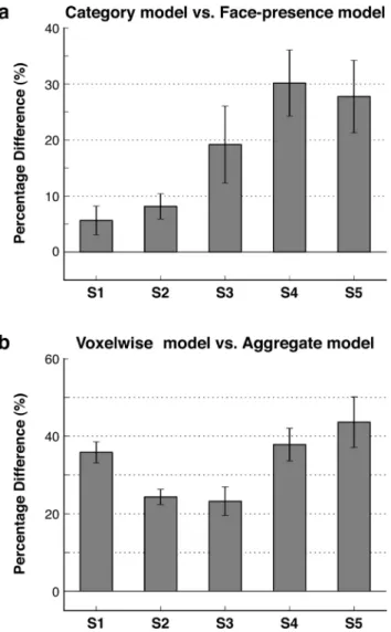
Control models. To assess the significance of FFA responses for nonface categories, a voxelwise face-presence model was fit to the BOLD re-sponses using the procedures described above. The face-presence model contained three separate regressors to account for graded degrees of face presence in the movies. These regressors coded the presence of primary faces (a face is the main object in the movie, and it is highly salient), secondary faces (a face is not the main object, but viewers are likely aware of its presence), and tertiary faces (a face is not the main object, and viewers are likely unaware of its presence). Primary faces were present in 600 s, secondary faces were present in 3560 s, and tertiary faces were present in 465 s of the movies. The full category model was compared with the face-presence model in terms of the proportion of response variance explained in the test data. Significance of differences in ex-plained variance was assessed using bootstrap tests.
To assess the significance of heterogeneous category tuning in FFA, a separate control analysis was performed using the full category model. First, the prediction score for each voxel was calculated separately using each voxel’s own model. Then, the models for the remaining voxels were used to generate response predictions for the held-out voxel, and these predictions were averaged. Each voxel’s own model was compared with the average of remaining models in terms of the proportion of response variance explained in the test data. Significance of differences in ex-plained variance was assessed using bootstrap tests.
A separate motion-energy model was used to assess selectivity for sim-ple visual features. It was shown in an earlier study that the motion-energy model accurately predicts voxel responses to natural movies in several retinotopically organized visual areas (Nishimoto et al., 2011). The motion-energy model consisted of 6555 spatiotemporal Gabor wavelet filters. Each filter was constructed by multiplying a 3D spatio-temporal sinusoid by a spatiospatio-temporal Gaussian envelope. Filters oc-curred at five spatial frequencies (0, 2, 4, 8, 16, and 32 cycles/image), three temporal frequencies (0, 2, and 4 Hz), and eight directions (0, 45 . . . 315 degrees). Filters were positioned on a square grid that covered the movie screen. Grid spacing was determined separately for filters at each spatial frequency so that adjacent Gabor wavelets were separated by 3.5 SDs of the spatial Gaussian envelope.
Clustering analysis
Preliminary inspection of the category tuning profiles revealed a rela-tively heterogeneous distribution of category selectivity among FFA vox-els. Hence, a data-driven clustering approach was adopted to unveil intrinsic group structure among these voxels. All analyses were repeated for multiple FFA definitions based on varying p value thresholds.
Spectral clustering. A spectral clustering algorithm was used that usu-ally offers more reliable performance than traditional techniques (Ng et
al., 2001;Zelnik-Manor and Perona, 2004). The spectral clustering algo-rithm first forms a fully connected affinity graph G⫽ (V, E) with vertices corresponding to individual tuning profiles. The edges connecting these vertices are assigned non-negative weights, W, that represent the affinity between the curves. Here, we used a reliable self-tuning affinity measure as follows: Wij ⫽
再
e⫺dij 2/ 2 ij, i ⫽ j 0 , i ⫽ j (1)whereidenotes the scale parameter equal to the average distance
be-tween the curve for the ithvoxel and the curves for all other voxels
(Zelnik-Manor and Perona, 2004).
Figure 2. Significance of tuning for nonface categories and of heterogeneous category tun-ing. a, Separate voxelwise face-presence models were fit to assess the significance of tuning for nonface categories. The face-presence model captured responses to the graded presence of faces in the movies (see Materials and Methods). The full category model (i.e., including 1705 categories) was compared with the face-presence model in terms of response predictions. Bar plots show the percentage difference in explained variance across the population of FFA voxels for subjects S1–S5 (mean⫾ SEM). The full model increases the explained variance in each subject ( p⬍ 10⫺4, bootstrap test). This result indicates that tuning for nonface categories is significant. b, A separate control analysis was performed to assess the significance of heteroge-neous category tuning within FFA. The full category model for each voxel was compared with an aggregate model obtained by averaging the voxelwise models across the remaining voxels. Bar plots show the percentage difference in explained variance across the population of FFA voxels for subjects S1–S5 (mean⫾ SEM). The voxelwise models increase the explained variance in each subject ( p⬍ 10⫺4, bootstrap test). This result indicates that the heterogeneity of cate-gory tuning among FFA voxels is significant.
Afterward, spectral clustering attempts to partition the graph such that the resulting clusters are as weakly connected as possible (i.e., the
connecting edges have low weights) (Luxburg, 2007). Ideally, each
cluster denotes a subset of vertices that are connected to each other by a series of edges and disjoint from the remaining vertices in the graph. Such clusters can be found by computing the eigenvalue decomposi-tion of the graph Laplacian matrix, L僆 Rn⫻nwhere n is the number of
voxels (Ng et al., 2001). This matrix has as many zero-valued eigen-values as there are clusters in the partitioned graph. The correspond-ing eigenvectors indicate the vertices grouped in each connected cluster.
For a given number of clusters k, the clustering algorithm retrieves the eigenvectors corresponding to the k smallest eigenvalues, and appends
them to form a new matrix U僆 Rn⫻k. This dimensionality-reduced
representation emphasizes the group structure in the data, such that the next step of the spectral clustering algorithm, a simple k-means clustering applied on the rows of U, can trivially detect the clusters (MacQueen, 1967). Because k-means clustering can be sensitive to the choice of initial cluster centers, the clustering analyses were performed with 20 different random initializations. The initialization that yielded the lowest sum-of-squares of within-cluster distances was selected as the optimal solution. This procedure was repeated 10 times, and it was observed that 20 ran-dom initializations are sufficient to obtain the same optimal solutions across repetitions.
Distance function. Similar to many other clustering methods, spectral clustering requires the selection of a distance function to characterize the dissimilarity between the data points. A correlation-based measure was used to quantify the distance between pairs of tuning profiles (DeAngelis et al., 1999):
dij ⫽ 1 ⫺
ai 䡠 aj
储ai储 储aj储
(2) Here, dijis the distance between tuning profiles of voxels i, j, ai, and ajare the corresponding 1705-dimensional vectors denoting the tuning pro-files,储䡠储 indicates the l2-norm, and䡠 is a dot-product operation.
Number of clusters. Finding the optimum number of clusters is an important parameter selection problem for many clustering algorithms. A stability-based validation technique was used to quantitatively assess the quality of the clustering results, and to rationally determine the num-ber of clusters without relying on external information (Ben-Hur et al., 2002;Handl et al., 2005). This technique performs clustering analyses on subsamples of the data, and uses pairwise similarities between the clus-tering solutions as a measure of stability. Different numbers of clusters are then compared through their corresponding distributions of cluster-ing stability.
For different numbers of clusters k (1,2. . . 7), a separate jackknifing procedure was performed with 5000 iterations to estimate the prob-ability distribution of stprob-ability. (No computations were required for k⫽ 1, as the tuning profiles will always be placed in the same cluster.) At each iteration, 80% of the curves were randomly drawn twice, and spectral clustering was performed separately on these two sub-samples. The clustering results for the common set of curves included in both subsamples were characterized with labeling matrices, C as follows:
Cij ⫽
再
1, aiand ajare in the same cluster & i ⫽ j
0, otherwise (3) 0
Differences
Similarity CDFs
0 0.2 0.4 0.6 0.8 1 0.2 0.4 0.6 0.8 1 1 2 3 4 5 6 0 0.9 Number of clusters (k) Similarity (J)a
0 0 0.2 0.4 0.6 0.8 1 0.2 0.4 0.6 0.8 1 1 2 3 4 5 6 0 0.9 Number of clusters (k) Similarity (J)b
0 0 0.2 0.4 0.6 0.8 1 0.2 0.4 0.6 0.8 1 1 2 3 4 5 6 0 0.9 Number of clusters (k) Similarity (J) FJ (j ) ∆ FJ (j = 0.8)c
0 0 0.2 0.4 0.6 0.8 1 0.2 0.4 0.6 0.8 1 1 2 3 4 5 6 0 0.9 Number of clusters (k) Similarity (J)d
0 0 0.2 0.4 0.6 0.8 1 0.2 0.4 0.6 0.8 1 1 2 3 4 5 6 0 0.9 Number of clusters (k) Similarity (J)e
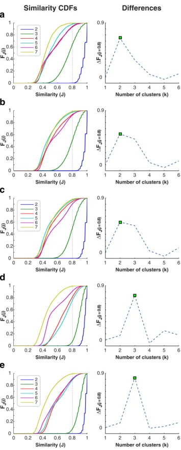
FJ (j ) ∆ FJ (j = 0.8) FJ (j ) ∆ FJ (j = 0.8) FJ (j ) ∆ FJ (j = 0.8) FJ (j ) ∆ FJ (j = 0.8) 2 3 4 5 6 7 2 3 4 5 6 7 2 3 4 5 6 7Figure 3. The number of clusters. A stability-based validation technique was used to deter-mine the optimal number of clusters for multiple FFA definitions based on varying localizer thresholds: a, p⬍1⫻10⫺6. b, p⬍5⫻10⫺6. c, p⬍1⫻10⫺5. d, p⬍5⫻10⫺5. e, p⬍ 1⫻ 10⫺4. For each FFA definition, the cluster stability was determined separately for several numbers of clusters (k). This validation technique measures the cluster stability against random perturbations in the dataset. Specifically, stability was measured as the similarity of clustering solutions that are performed on random subsamples (i.e., 80%) of FFA voxels pooled across subjects. The pairwise similarities (J) between the clustering solutions were histogrammed to generate the cumulative distribution functions (CDFs) shown in the left column. If the solutions are stable, then the distributions will be concentrated around 1. If the solutions are instead
4
unstable, the distributions will be widespread. Thus, the optimal number of clusters can be identified by a sudden transition from narrow to more widespread distributions. To detect such transitions, we calculated the percentage of similarity measurements that were below a high similarity threshold (i.e., J⬍0.8)foreachnumberofclusters.Thedifferencesinthispercentage value between consecutive numbers of clusters are plotted in the right column. The optimal number of clusters was determined as the point where the difference in maximized (green dot).
The similarity of the two clustering results, C(1)and C(2), were then
computed using the Jaccard Index (Jaccard, 1908):
J共C共1兲,C共2兲兲 ⫽ C
共1兲: C共2兲
C共1兲: C共1兲 ⫹ C共2兲: C共2兲 ⫺ C共1兲: C共2兲 (4) here “:” denotes the Frobenious innerproduct for matrices. The proba-bility distribution functions P( j) and thereby cumulative distribution functions FJ( j) were obtained by calculating the normalized histograms (with a bin width of 0.005) of 5000 similarity values.
Finally, the optimal number of clusters was determined from the re-sulting cumulative distribution functions (Ben-Hur et al., 2002). The optimal value can be identified by a sudden transition from distributions concentrated around a similarity of 1 (i.e., stable clustering solutions) to more widespread distributions (i.e., unstable clustering solutions). We used a quantitative rationale to detect such transitions as follows:
Rationale
For each distribution of similarity FJ( j)⫽ P(J ⬍ j), determine the value
of FJ(0.8)⫽ P(J ⬍ 0.8).
Compute the finite differences of these values across consecutive num-bers of clusters (k),⌬FJk⫽ FJk⫹1(0.8)⫺ FJk(0.8).
The optimal k is chosen to maximize the finite difference⌬FJk.
Unstable clustering solutions will generate more uniform distribu-tions of similarity, and P(J⬍ 0.8) will be relatively small. In contrast, stable solutions will have narrower distributions and yield higher P(J⬍ 0.8). Therefore, there will be a relatively big jump in P(J⬍ 0.8) values during the transition from stable to unstable solutions. This technique will successfully detect the absence of clusters in the data, as in this case the distributions for k⬎ 1 will all be considerably widespread.
Repeatability. By selecting the optimal number of clusters based on stability, a stringent criterion is enforced on the repeatability of the clus-tering results. This criterion assures that clusclus-tering labels are reliable against perturbations in the dataset. However, the stability of labels does not provide direct information about the variability in the cluster centers, which is critical for the interpretation of the results. Such variability may arise from the k-means step in spectral clustering that relies on random initializations. Therefore, the clustering analysis may potentially yield different cluster centers in each run.
To assess the repeatability of the cluster centers, the spectral clus-tering analysis was repeated 10,000 times using the entire dataset (instead of subsamples) and the optimal number of clusters deter-mined in the previous step. Apart from variations in the centers re-sulting from k-means, the cluster labels can also be randomly permuted in between iterations. Therefore, the corresponding cluster labels were matched by maximizing the overlap between the identities of the voxels assigned to each cluster. In other words, clusters that
shared the largest number of voxels were matched. The similarity between matched pairs of cluster centers were then quantified by correlation coefficients (Pearson’s r). Fi-nally, bootstrap tests were performed to de-termine whether these correlations were significantly above a stringent threshold of 0.95.
Visualization in model space
To interpret the results of the clustering analysis, the cluster centers were individually visualized with graphs in the model space. These graphs were constructed by plotting the objects and actions in our category model with separate tree structures. Each graph ver-tex was used to denote a distinct feature in the category model. Meanwhile, graph edges were used to represent the hierarchical WordNet relations between superordinate and subordinate categories. The locations of the vertices and the length of the edges were manually assigned for ease of visualization and do not convey informa-tion about semantic distances between categories. The size and color of the vertices indicate the magnitude and sign of the predicted responses to the corresponding categories, respectively.
Visualization on cortical flatmaps
To examine the organization of category representation across the cortex, flatmaps of the cortical surface were generated from anatom-ical data. The category tuning profiles were then visualized on cortanatom-ical flatmaps. For this purpose, a principal components analysis was first used to recover the dimensions of the semantic space represented by FFA. The tuning profile of each voxel was then projected into this semantic space. Statistical significance of the projections was evalu-ated using the null models generevalu-ated by the aforementioned Monte Carlo procedure (see Category encoding model). The null models for each voxel were also projected into the semantic space. To improve the quality of the semantic space, the analysis was restricted to the first
10 principal components that individually explain⬎1% of the
re-sponse variance. The category tuning of a voxel was deemed statisti-cally significant if its projection into the semantic space was significantly separated from the projections of the null models (2
test based on Mahalanobis distance). The significance levels were corrected for multiple comparisons using FDR control.
Spatial distribution of clusters
To examine whether FFA clusters are spatially segregated, spatial loca-tions of FFA voxels were measured separately in the volumetric brain spaces of each subject. If clusters are spatially segregated, pairwise dis-tances between voxels should be smaller for voxels within the same clus-ter than for voxels in different clusclus-ters. The distribution of within- versus across-cluster distances was measured separately for each cluster. This distribution was compared with a null distribution obtained by ran-domly assigning voxels to three clusters. Significance of spatial segrega-tion was assessed using bootstrap tests.
To assess characteristic differences in the spatial distribution of indi-vidual FFA clusters, two functional ROIs that lie along the ventral collat-eral sulcus (CoS) and middle temporal sulcus (MTS), namely, PPA and EBA, were used as spatial landmarks. Voxelwise spatial locations were measured separately in the volumetric brain spaces of individual sub-jects. The centers of PPA and EBA were obtained by averaging the spatial locations of entailed voxels. A reference direction that linearly traverses from the center of EBA to PPA was computed in the volumetric space. The spatial location of each FFA voxel was projected onto this reference direction. Voxels that are spatially closer to PPA should have larger pro-jections, and voxels that are spatially closer to EBA should have smaller projections. Significance of differences in spatial locations was assessed using bootstrap tests.
1.0 S1 S2 S3 All S1 S2 S3 All
Cluster 1
S5 S4 S4 S5 S1 S2 S3 All S1 S2 S3 AllCluster 2
S5 S4 S4 S5 0.0 -1.0 S1 S2 S3 All S1 S2 S3 AllCluster 3
S5 S4 S4 S5Figure 4. Similarity of cluster centers across subjects. To examine whether the functional subdomains within FFA are consistent across subjects, clustering analysis was performed for each subject individually. The cluster centers computed in individual subjects were compared across subjects and compared with the group cluster centers. Similarity measurements were performed between cluster centers estimated separately from responses to the first and second halves of the movies. FFA voxels were defined using a localizer threshold of p⬍ 10⫺4. The similarities (as measured by correlation) of cluster centers are displayed with separate matrices. The row and column labels identify the group (All) and individual-subject (S1, S2, S3, S4, and S5) cluster centers. The color scale ranges from black for negative correlation (⫺1)towhiteforpositivecorrelation(1).Thegroupandindividual-subjectcluster centers are quite similar (p⬍ 10⫺4, bootstrap test). This indicates that the functional heterogeneity within FFA is reliable for individual subjects and consistent across subjects.
Silhouette width
The separability of the identified clusters was calculated using the average silhouette width (Peter, 1987). This average width reflects the quality of clustering and is quantified as the mean of voxelwise silhouette widths Si:
Si ⫽ min Z⫽Zi 共dij兲j⑀Z ⫺ 共d ij兲j⑀Zi max
冉
minZ⫽Zi 共dij兲j⑀Z,共d ij兲j⑀Zi冊
(5)Here Z denotes the set of voxels assigned to a given cluster and Zidenotes
cluster label for the ithvoxel.共d
ij兲j⑀Zis the average distance between the ith
voxel and all voxels in cluster Z.
Results
Category tuning of FFA voxels
The human FFA is commonly assumed to be involved in category
representation (
Kanwisher, 2010
). To measure FFA tuning for
hundreds of object and action categories, we fit separate category
u moveo ev m m ve jump j mum jump walk w travelavv t v travellel ungulateguuululla ung pedestrianrii p estriaiann talk ta communicatemunmumununicat carnivore carn re placental pl p en p place l pl rodent gesture groupuup athletet ath ath measure m colorllol r clo c
attributetritriibuiuteuute a iu a ue athmosphericth phenomenonhehhenh pp eventent e e e t ee persone so peerersonsosoon p pe persson organismn org birdddd bir b planta pl womanmananan childhi dilddddd chil road ro ro roooo
artifactrtifactiittiiffafacta
weapon objectobjojeecct
body bodd body bd part pa pa parrt prtyy truck motorcycley car airplanee ship
instrumentalityrumrumemennn lity i tr n y ins mnnt boat wheeled vehicle equipmentquqququuiipppm t eqippmpp nt structure ss uu stru ttucturu uuccctu s building b b b b b dooro room r ro ro grassland location looocaocati city beveragev aggegege sky water waat face material matterter ma desertsserses t prairieee parkingkingg lototttt clothingotthinggg furnitureni driving d i d communicationmuu catioaattitiio animalim devicee icvi dev cev e d deev de
containerntta naaineaiiinn
geological ge geooogo geolo formationo foor n fo g g g g g g g g vehicle turnu moveo ev m m ve jump j mum jump walk w wa travelavv t v travellel t ungulateguuul unula ug pedestrianrii na p striann talk ta communicatemumunuunicatt
carnivore carn placental p pla p en p pa l p rodent gesture grouprup athleteth at measure m colorlol r c o clo co attributetritribuiutuute aribu a ute athmosphericth phenomenonhhehen ph pp eventent e e eet eve person p serssso peer onsosoon p pe pers n organismn org birdid plant p an pl womanmananan childhildldlddddd road rro rod ro dd roa
artifactrtitifactiffaiffaiiffactt ar
weapon objectobjoobjeectcct
body bododyd bdy part pa pa part prtyy truck motorcycley car airplanee ship
instrumentalitytrrumrumemenen lityy inst m ntn boat wheeled vehicle equipmentqqququuiippp tt eqippmpp nt structure s utrtrru ureuccturctttuur st buildingi b b bu doororr room r ro ro r grassland location looocaati llooc cityy cii c beveragev agggege skyyy water waat face materialt matterter ma desertsserses tt d rt prairieee parkingrkingg lotoottt clothingotthinggg furnitureurnitur driving d i d di communicationmu ca iaattitiio animali devicee icvi dev ceve d deev de
containernntttta ntaaaiiiinnen c geological ge g oeoog geolo formation form n fo f g g g g g g g vehicle turnu moveo ev m m ve jump j mum j mpu walk w wa travelavv t v travellel t el ungulateguuululla ung pedestrianrii p estriaiann talk ta communicatemumunuunicat carnivore carn ore placental pl p en p place l pl rodent r gesture grouprup athletet ath ath measure m colorllol r cl
attributetritriibuiuteuute a i e athmosphericth phenomenonhehhenh pp eventent e e eet eve persone sos peerersonsosoon p pe persson organismn org birdddd bir b planta pl womanmananan
childhildildddddd ch l road rro roo ro roa
artifactrtifactiittiiffafacta
weapon objectobjojeecctc
body bododyyd b dy part part parrttyyy truck motorcycle car airplanee ship
instrumentalityrumrumemennn lity i r n in nt boat wheeled vehicle equipment eququq puiipppm t structure ss utru ttucturuuccctutu s building b b b b dooro room r r grassland location looocaati loc cityy c beverageaggegege sky water waat face material matterter ma desertsserses t prairiee parkingkingg lotottttt clothingthinngg furniturenin driving d i d communicationmu catioattittiio animalnimm deviceevvicvi dev cev e d dev
containerntta nnaaainain
geological ge geoooog geolo formationo form n fo g g g g g g g g vehicle
a
Cluster 1
b
Cluster 2
+
-Below Mean Above Mean P re dic ted Response
c
Cluster 3
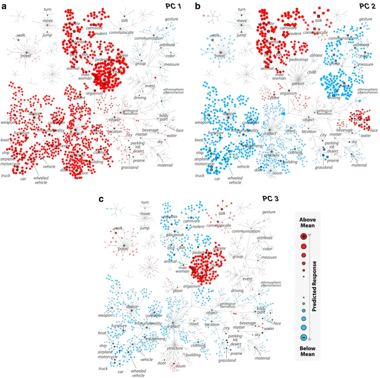
Figure 5. The cluster centers. Spectral clustering analysis among FFA voxels reveals three functional subdomains. a– c, Mean tuning profiles across voxels within each cluster are shown using a series of graphs for object (main tree, circular vertices) and action (smaller trees, square vertices) categories. Subsets of the categories are labeled to orient the reader. The size of each vertex indicates the magnitude, whereas its color indicates the sign (red represents⫹; blue represents ⫺) of the category response (see legend). a, Responses of the first cluster are strongly enhanced by humans and animals and weakly enhanced by man-made instruments, including vehicles ( p⬍ 0.05, Monte Carlo test, FDR corrected). b, Responses of the second cluster are strongly enhanced by humans and animals ( p⬍ 0.05) and weakly enhanced by body parts and communication verbs, including primary faces (faces that are the most salient object in the scene). c, Responses of the third cluster are strongly enhanced by humans, placental mammals, communication verbs, gestures (i.e., facial gestures), and faces but strongly suppressed by man-made artifacts, particularly structures, such as buildings and rooms ( p⬍ 0.05). Responses of all three clusters are suppressed by many natural objects, such as geological landscapes and natural materials (p ⬍ 0.05).
models to single FFA voxels in each individual subject (
Fig. 1
).
FFA definitions were obtained from functional localizer data by
first removing voxels with a positive body-versus-face contrast
and then applying varying p value thresholds to a
face-versus-object contrast (see Materials and Methods). We find that the
category models provide significant response predictions for all
FFA voxels ( p
⬍ 10
⫺4, jackknife test, FDR corrected).
Evidence from several fMRI studies implies that FFA might be
differentially tuned for nonface objects (
O’Toole et al., 2005
;
Reddy and Kanwisher, 2007
;
Huth et al., 2012
). If FFA exhibits
tuning for nonface categories, then nonface category responses
should account for a significant portion of the total response
variance in FFA voxels. To assess whether FFA is significantly
tuned for nonface categories, we performed two complementary
analyses. First, we separately fit a face-presence model to each
FFA voxel that captured responses to the graded presence of faces
in the movies (see Materials and Methods). We reasoned that, if
nonface category responses are significant, the full category
model should yield better predictions of the BOLD responses
than the face-presence model.
Figure 2
a shows the difference in
variance explained by the full category model versus the
face-presence model. We find that the proportion of explained
vari-ance across FFA voxels is R
2⫽ 0.359 ⫾ 0.070 (mean ⫾ SD across
subjects) for the full category model and R
2⫽ 0.308 ⫾ 0.074 for
the face-presence model. The average improvement in explained
variance across the population of FFA voxels is 18.2
⫾ 9.6%
(mean
⫾ SD across subjects). In every subject, the difference in
explained variance is significant ( p
⬍ 10
⫺4, bootstrap test). Thus,
tuning for nonface categories accounts for a significant and
sub-stantial part of the response variance in FFA.
Next, we performed a separate analysis to ensure that the
ad-ditional response variance explained by the full category model
over the face-presence model is not an artifact of scenes that were
correlated with the presence of faces. For this purpose, we refit the
full category model after removing all training data (including a
6 s safety margin to account for hemodynamic delays) collected
while humans, animals, or body parts were present in the movies
regardless of face presence. We reasoned that, if the difference in
explained variance between the category and face-presence
mod-els is the result of nonface category responses, then the category
model fit to face-absent data should explain a comparable
pro-portion of variance to this difference. Indeed, we find that the
proportion of variance explained by the category model fit to
face-absent data is R
2⫽ 0.058 ⫾ 0.034 (mean ⫾ SD across
sub-jects; p
⬍ 10
⫺4, bootstrap test), which is
nearly identical to the additional variance
explained by the category model fit to all
training data (
⌬R
2⫽ 0.051 ⫾ 0.021,
mean
⫾ SD). This finding affirms that
FFA tuning for nonface categories is not
an artifact of subjective face percepts.
One recent fMRI study proposed that
category tuning might be heterogeneously
distributed across voxels within FFA
(
Grill-Spector et al., 2006
). If FFA exhibits
spatially heterogeneous category tuning,
then intervoxel differences in category
re-sponses should account for a significant
portion of the total variance in FFA
vox-els. In turn, this would imply that each
voxelwise model should yield better
pdictions of that particular voxel’s
re-sponses compared with an aggregate
model averaged across the remaining voxels.
Figure 2
b shows the
difference in variance explained by each voxel’s own model
ver-sus the average FFA model. We find that the proportion of
ex-plained variance across FFA voxels is R
2⫽ 0.359 ⫾ 0.070
(mean
⫾ SD across subjects) for each voxel’s own model and R
2⫽ 0.266 ⫾ 0.049 for the average FFA model. In every subject, the
voxelwise model explains significantly more variance than the
average FFA model ( p
⬍ 10
⫺4, bootstrap test). The average
im-provement in explained variance across the population of FFA
voxels is 34.4
⫾ 4.6% (mean ⫾ SD across subjects). This
im-provement cannot be attributed to simple response baseline or
gain differences among FFA voxels because BOLD responses of
each voxel were individually z-scored before modeling and
be-cause prediction scores were measured using correlation. Thus,
this result demonstrates that differences in category tuning
among FFA voxels account for a significant portion of FFA
re-sponses.
Clustering analysis
To systematically assess variations of category tuning within FFA,
we used spectral clustering to analyze voxelwise tuning profiles in
individual subjects. A stability-based technique was used to select
the optimal number of clusters (k) without relying on external
information (see Materials and Methods for details). The optimal
k was determined separately for each FFA definition based on
varying localizer thresholds. We find that the FFA voxels fall into
three distinct clusters for every subject, even at stringent
thresh-olds (starting with p
⬍ 5 ⫻ 10
⫺5; see
Table 1
). Even at
exceed-ingly stringent thresholds down to p
⬍ 10
⫺10, FFA voxels fall into
two distinct clusters. Typical thresholds used to define FFA in
previous studies range from 10
⫺5to 10
⫺3(
Spiridon and
Kan-wisher, 2002
;
Grill-Spector et al., 2006
;
Reddy and Kanwisher,
2007
). To increase the sensitivity in verifying the optimal number
of clusters, we repeated the stability-based validation at the group
level after pooling FFA voxels across subjects. We find that the
FFA voxels fall into three distinct clusters at the group level,
con-sistent with the results obtained at the level of individual subjects
(
Fig. 3
). These results indicate that FFA has at least three
func-tional subdomains for category tuning.
To examine the consistency of FFA subdomains across
sub-jects, we compared the category tuning of the voxel clusters
iden-tified in separate subjects. The category tuning of each cluster was
taken as the mean tuning profile across FFA voxels within the
cluster (i.e., the cluster center). The stability of the cluster centers
Figure 6. Response levels to object and action categories in each cluster. The responses of each cluster to eight distinct categories were computed, including humans, animals, body parts, communication, vehicles, structures (e.g., building, room), natural materials (e.g., water, soil), and geographic locations (i.e., mountain, city). The response to each category was computed as the mean response to all of its subordinate categories. Individual voxel responses were averaged within each cluster to compute the average category responses (mean⫾ SEM, across voxels within each cluster). The first cluster is broadly tuned for humans, animals, and vehicles. The second cluster is tuned for humans and animals. Finally, the third cluster is tuned for humans, body parts, and communication.
was first evaluated using a bootstrap procedure (see Materials
and Methods). We find that all three cluster centers are highly
stable and repeatable in individual subjects ( p
⬍ 10
⫺4, bootstrap
test). The cluster centers were then compared across subjects. We
find that the cluster centers are highly correlated across subjects
(r
⫽ 0.73 ⫾ 0.15, mean ⫾ SD across subjects, p ⬍ 10
⫺4, bootstrap
test). We also find that the within-cluster correlations are
higher than the across-cluster correlations (
⌬r ⫽ 0.13 ⫾ 0.04,
p
⬍ 10
⫺4).
To facilitate intersubject comparisons and increase sensitivity,
we repeated the clustering analyses at the group level. We find
that all three group cluster centers are highly repeatable ( p
⬍
10
⫺4, bootstrap test) and that they are highly correlated with
individual-subject cluster centers (r
⫽ 0.86 ⫾ 0.15, mean ⫾ SD
across subjects, p
⬍ 10
⫺4, bootstrap test).
To ensure that intersubject consistency of the clusters is not
biased by spurious correlations in the movies, we also measured
the similarity of cluster centers estimated separately from
re-sponses to the first and second halves of the movies. We find that
the split-half cluster centers are highly correlated across subjects
(
Fig. 4
; r
⫽ 0.65 ⫾ 0.14, mean ⫾ SD, p ⬍ 10
⫺4, bootstrap test)
and with the group cluster centers (r
⫽ 0.73 ⫾ 0.14, mean ⫾ SD).
Together, these results suggest that functional heterogeneity
among FFA voxels is reliable for individual subjects and
consis-tent across subjects.
Finally, to reveal the aspects of category information that are
represented in each cluster, we assessed the differences in
cate-gory tuning across the clusters. For this purpose, we inspected the
three group cluster centers obtained when FFA was defined using
a localizer threshold of p
⬍ 10
⫺4(
Fig. 5
; see
Fig. 13
for
individual-subject cluster centers; see
Fig. 14
for raw model weights of the
group cluster centers). To highlight the key differences between
the cluster centers, we compared the average response levels of
each cluster with several important object and action categories
(
Fig. 6
). BOLD responses of the first cluster are strongly enhanced
by humans and animals and weakly enhanced by man-made
in-struments, including vehicles ( p
⬍ 0.05, Monte Carlo test, FDR
corrected). Responses of the second cluster are strongly enhanced
by humans and animals ( p
⬍ 0.05) and weakly enhanced by
communication verbs and body parts, including primary faces
(faces that are the most salient object in the scene). Responses of
the third cluster are strongly enhanced by humans, placental
mammals, communication verbs, gestures (i.e., facial gestures),
and faces but strongly suppressed by man-made artifacts,
partic-ularly structures, such as buildings and rooms ( p
⬍ 0.05).
Re-sponses of all three clusters are suppressed by many natural
objects, such as geological landscapes and natural materials ( p
⬍
0.05). These results suggest that the clusters in FFA are broadly
tuned for many nonface categories, and differ in their tuning for
these nonface categories.
2
S
1
S
4
S
3
S
S5
Cluster 1
Cluster 2
Cluster 3
anterior posterior left rightFigure 7. Spatial distribution of clusters. The spatial distribution of clusters shown in the volumetric brain spaces of individual subjects (S1–S5). FFA voxels were defined using a localizer threshold of p⬍ 10⫺4. Separate clusters are labeled with blue, green, and red colors overlaid onto anatomical images (see legend). Consecutive axial slices at the ventral occipitotemporal areas are grouped in montage format. The clusters are spatially segregated in the brain space of each subject ( p⬍10⫺5for S1–S3 and S5, p⬍0.02forS4,bootstraptest).Thefirstclusterthathasthestrongesttuning for instruments, vehicles, and structures among the three clusters is located anteriorly relative to the remaining clusters, and closer to regions along the ventral collateral sulcus that are assumed to be selective for scenes with man-made structures ( p⬍ 10⫺4, bootstrap test). The second cluster that has the strongest tuning for humans and animals is located posteriorly and closer to regions along the middle temporal sulcus that are known to be selective for animate motion and bodies ( p⬍ 10⫺4). Last, the third cluster that has the strongest tuning for communication verbs and human body parts and weakest selectivity for animals is located centromedially ( p⬍ 10⫺4). There is no significant hemispheric lateralization for any of the three clusters ( p⬎ 0.34, bootstrap test).