An integer programming based algorithm for the resource constrained project scheduling problem

(1)

İm m M İîi

м ш

í

.

íssísw m ш ■№! Ж Ѣ Ш Ш â t t î ü ; . . . - - · - ? » İ C T K i ä t t J Ä S J Ï ^ O B iS i *■*« i . i Z ^ ¡ 3 -V Л ^^''ilTT^D .ам il J M i< \¡J t. mMt *ni>'» -MM* ~ Ы ·.. 4 v m . · r* w < . ».« Т У /S '? * 5

•Я 83

(2)

AN INTEGER PROGRAMMING BASED ALGORITHM FOR THE RESOURCE CONSTRAINED PROJECT SCHEDULING PROBLEM

A THESIS

SUBMITTED TO THE DEPARTMENT OF INDUSTRIAL ENGINEERING

AND THE INSTITUTE OF ENGINEERING AND SCIENCES OF BILKENT UNIVERSITY

IN PARTIAL FULFILLMENT OF THE REQUIREMENTS FOR THE DEGREE OF

MASTER OF SCIENCE

By

İsmet Esra Büyüktahtakın January 2005

(3)

Jb;

.1 <Г5 ’ D . 8

T

О

(4)

I certify that I have read this thesis and that in my opinion it is fully adequate, in scope and in quality, as a thesis for the degree of Master of Science.

I certify that I have read this thesis and that in my opinion it is fully adequate, in scope and in quality, as/a thesis for/(he degree of Master of Science.

isst. Prof Mu at Fadiloglu

\

Approved for the Institute of Engineering and Sciences:

Prof Mehmet Baray y ' ,

Director of Institute of Engineering and Sciences

(5)

ABSTRACT

AN INTEGER PROGRAMMING BASED ALGORITHM FOR THE RESOURCE CONSTRAINED PROJECT SCHEDULING PROBLEM

İsmet Esra Büyüktahtakm M.S. in Industrial Engineering Supervisor: Assoc. Prof. Osman Oğuz

January 2005

In this thesis, we study the problem of scheduling the activities of a single project in order for all resource and precedence relationships constraints to be satisfied with an objective of minimizing the project completion time. To solve this problem, we propose an Integer Programming based approximation algorithm, which has two phases. In the first phase of the algorithm, a subproblem generation technique and enumerative cuts used to tighten the formulation of the problem are presented. If an optimal solution is not found within a predetermined time limit, we continue with the second phase that uses the cuts and the lower bound obtained in the first phase. In order to evaluate the efficiency of our algorithm, we used the benchmark instances in the literature and compared the results with the best known solutions available for these instances. Finally, the computational results are reported and discussed.

Keywords: Project Management, Scheduling, 0-1 Integer Programming

(6)

ÖZET

KAYNAK KISITLI PROJE ÇİZELGELEME PROBLEMİ İÇİN TAMSAYI PROGRAMLAMA TABANLI BİR ALGORİTMA

İsmet Esra Büyüktahtakm Endüstri Mühendisliği, Yüksek Lisans Tez Yöneticisi: Doç. Dr. Osman Oğuz

Ocak 2005

Bu tezde, bir projenin faaliyetlerini tüm kaynak ve ön ilişkiler kısıtlayıcılarını sağlayacak ve projenin bitiş zamanını enazlıyacak şekilde çizelgeleme problemini çalıştık. Bu problemi çözmek için iki fazlı tamsayı programlama tabanlı bir yaklaşıklama algoritması önerdik. Algoritmanın ilk fazında alt problem üretme tekniği ve problem formulasyonunu sıkılaştıraıak için kullanılan birerleyici kesmeler sunulmuştur. Önceden belirlemniş bir zaman limiti içinde eniyi çözüm bulunamaması halinde, ilk fazda üretilmiş kesmeleri ve alt sınırı kullanan ikinci faza geçilir. Algoritmamızın etkinliğini değerlendirebilmek amacıyla literatürdeki denektaşı niteliğindeki problemleri kullandık ve sonuçları bu problemlerin mevcut en iyi çözümleriyle kıyasladık. Son olarak, hesaba dayalı sonuçlara ve değerlendinnelere yer verilmiştir.

Anahtar Kelimeler: Proje Yönetimi, Çizelgeleme, 0-1 tamsayıh programlama

(7)

(8)

ACKNOWLEDGEMENT

I would like to express my sincere gratitude to Assoc. Prof. Osman Oğuz for his supervision and encouragement during my graduate study. His endless patience, understanding and guidance let this thesis come to an end.

I am indebted to Assoc. Prof Oya Ekin Karaşan, Asst. Prof Hande Yaman and Asst. Prof Murat Fadıloğlu for accepting to read and review this thesis and for their valuable comments and suggestions.

I would like to express my sincere thanks to Hayriye Çiçekçi for her friendship, encouragement and love.

I would like to take this opportunity to thank Duygu Pekbey, Mustafa Rasim Kılıç, Ayşegül Altın, Hakan Gültekin, Kürşad Derinkuyu and Mehmet AjTancı. I cannot forget their help and valuable support throughout this thesis work.

I would like to thank to Adife Yapça, Ağcagül Yılmaz, Zümbül Bulut, Gökhan Metan, Mehmet Oğuz Atan, Yasin Göçgün, Emrah Zarifoğlu and Banu Yüksel for their friendship and morale support. I am also thankful to my officemates and to all Industrial Engineering Department staff

Though I cannot list all of their names, there is a group of friends to whom I would also like to express my appreciation for their friendship and support.

Finally, I would like to express my deepest gratitude to my family. To my father Adem Büyüktahtakm for his encouragement, understanding, and confidence, to my mother Ayşe Büyüktahtakm and my brothers Ibrahim and Ömer Büyüktahtakm for their love and understanding. I feel lucky to have such a wonderful family, and without them the completion of this thesis would be impossible.

(9)

C O N T E N T S 1 INTRODUCTION 1 2 LITERATURE REVIEW 3 2.1 Optimization Procedures ... 4 2.1.1 Integer Programming... 4 2.1.2 Implicit Enumeration...6

2.1.3 Branch and Bound Techniques...7

2.2 Heuristic Approaches... 11

3 PROBLEM FORMULATION AND SOLUTION PROCEDURE 19 3.1 Problem Fonnulation...19

3.2 Algorithm...23

3.2.1 First Phase of the Algoritlim... 24

3.2.2 Second Phase of the Algorithm...29

3.3 An example... 31

3.4 Remarks...35

(10)

CONTENTS 4 COMPUTATIONAL RESULTS 4.1 Test Data, 36 ..36 4.2 Computational Results... 38

5 CONCLUSIONS AND RECOMMENDATIONS 45

BIBLIOGRAPHY 48

(11)

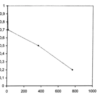
3.3: Example test problem with scheduling results... 31 4.2a: Increase in average CPU time as RS decreases with NC=1.5 and RF=0.25

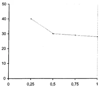
for J60...42 4.2b: Decrease in average number of problems solved to optimality as RF

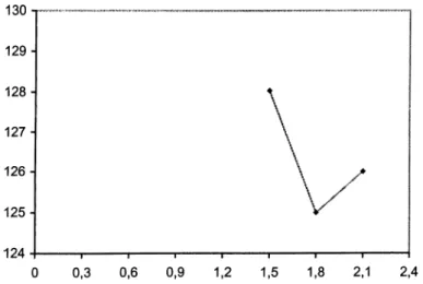
increases for N=30...43 4.2c: The change in average number of problems solved to optimality when

NC=1.5, NC=1.8 and NC=2.1 for J30... 44

L I S T O F F I G U R E S

(12)

L IS T O F T A B L E S

3.3: The integer values of the selected variables as part of the MIP relaxation

solution in each iteration...32

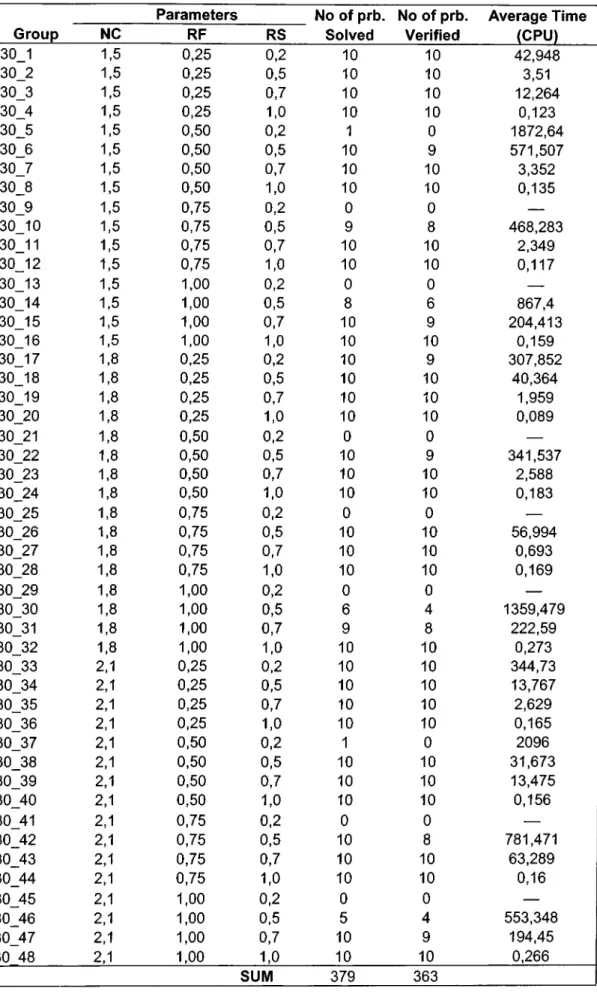
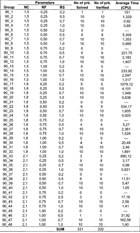
4.2a: PROGEN instances with N=30 and R=4...39

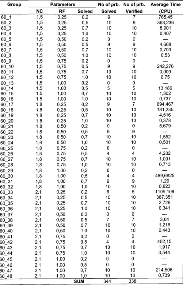
4.2b: PROGEN instances with N=60 and R=4... 40

(13)

Chapter 1 Introduction

The resource constrained project scheduling is a very popular research topic that has attracted wide interest of both practitioners and researchers. Its importance stems from its applications in diverse areas such as production planning and control, software development, and construction engineering. The resource constrained project scheduling problem (RCPSP) is beautifully formulated as an integer program; unfortunately its exact solution is almost impossible to find due to the fact that it is NP-complete (Blazewicz et al., 1983).

The popularity of project scheduling has been on the rise since the development of PERT (program evaluation and review technique) and CPM (critical path method) techniques in the mid 1950s. The major drawback of the CPM/PERT techniques is that these procedures do not provide feasible schedules for many real life projects since they assume that there is an infinite amount of resources available for each activity in the project network. With the introduction of the resource constraints, the problem becomes an NP-hard optimization problem and requires more advanced optimization techniques to be solved.

(14)

The research on resource constrained project scheduling problem has grown on various directions. Different versions of this problem can be classified according to the number of simultaneously scheduled projects (single, multiple), the nature of the optimizing objective function, the nature of resources and the activities in the project (Boctor, 1990). In this study we will focus on the classical resource constrained project scheduling problem in which the activities of a single project is scheduled subject to precedence and resource constraints with respect to the makespan minimization objective. Our problem is denoted by PS \prec \ C„,ax in the notation of Brucker et. al. (1999).

There are quite a few methods in the literature for solving the general RCPSP as a zero-one integer programming problem. The major drawback of these models is the excessive number of binary variables and constraints that make the problem computationally intractable. Many researchers such as Huber (1974) and Patterson (1984) conclude that zero-one programming is not an effective means of solving this problem since the early attempts at using IP to solve the exact version of this problem were unsuccessful. Therefore integer programming is not considered as an alternative for solving the RCPSP by many researchers. In our study we aim to show that with the appropriate cuts applied to the problem formulation, good results can be obtained in reasonable computational times. We present the enumerative cuts and a two phased approximation algorithm using Cplex as an IP solver and investigate the perfomiance of our algorithm, which is based on Integer Programming.

CHAPTER 1. INTRODUCTION 2

The thesis is organized as follows: In Chapter 2, a literature review for the classical resource constrained problem is provided. In Chapter 3, the problem formulation, the algorithm and an example problem are given. In Chapter 4, problem data and computational results are presented. Finally, some conclusions and remarks for future works are stated in Chapter 5.

(15)

Chapter 2 Literature Review

The solution techniques proposed for RCPSP can be divided into two major categories;

i. Optimization techniques that lead to the best schedule. These techniques are mathematical programming (linear, integer and dynamic programming) and enumeration approaches such as implicit enumeration and branch & bound.

ii. Heuristic or approximation approaches that will not lead to the optimal but good resource-feasible schedules.

For comprehensive reviews we refer the reader to Davis (1973), Herroelen et. al. (1997), Patterson (1984), Icmeli et. al. (1995), Elmaghraby (1995), Ozdamar and Ulusoy (1995) and Brucker et. al. (1999). Below we review exact and heuristic algorithms designed to solve the classical resource constrained project scheduling problem (RCPSP).

(16)

2.1 Optimization Solution Procedures:

2.1.1 Integer Programming

Pritsker et. al. (1969) propose an effective 0-1 integer programming formulation for the RCPSP. Their formulation is superior to the other known formulations in terms of computational tractability since it requires fewer variables and constraints to represent each scheduling problem. It is also a more general formulation, which can deal with the real life situations with three different objectives: the total throughput time minimization for all projects, makespan minimization and total lateness minimization. The fonnulation of Pritsker et. al. (1969) precedes and inspires the studies of Patterson and Huber (1974), Patterson and Talbot (1978), Talbot (1982) and many researchers use the various adaptations of this 0-1 formulation to represent the project scheduling problem they consider in their study. It is known that the major drawback of this formulation is that this formulation can only be used for very small problems since the number of variables increases very rapidly with the problem size. In our study, we used the modified version of this formulation with the makespan minimization objective and showed that this formulation could be used not for only small size problems but also for large size problems.

CHAPTER 2. LITERATURE REVIEW 4

Deckro et. al. (1991) propose a decomposition approach to solve the resource constrained multi-project scheduling problem. They model the problem as a block angular general integer program. They exploit the block angular structure of the general multi-project resource constrained problem by using the Sweeney-Murphy decomposition approach, which is a Lagrangean approach to solve the classical block-angular problem. By using this approach, they decompose the problem into a master problem, which is a linear program formed by the resource constraints and non-resource constrained single project sequencing problems fanned by the individual project constraints. The feasible solutions to the subproblems are used in the objective function of the master

(17)

problem. Since not all of the best solutions to each subproblem are used, the master problem is a restriction of the original problem thus the optimal solution of the restricted problem is not necessarily the optimal solution of the original problem. To overcome this problem, an optimality test is used. The authors report that the decomposition approach offers a computationally feasible procedure to solve large and complex multi-project, resource constrained problems.

Icmeli and Rom (1996) present three new models in which they relax the integrality assumption by imposing continuous activity durations, continuous resource consumption and continuous project life span. The resource availability assumptions differentiate each of these models. In the first model the resource availabilities are assigned to specific time milestones, which divide the project life span into some predetermined intervals whereas in the second, the resource availabilities are allocated to time intervals. However, in the third model, each activity is forced to start and end in the same interval and the resource availabilities are allocated to the time intervals. Two possible objective functions are used in the model: minimizing the makespan of the project and maximizing the net present value of the project cash flows. They use Optimization Subroutine Library from IBM to solve these models. They report a detailed analysis on a total of 1400 problems with different parameter settings to determine the factors that affect the computational efficiency of the code and the models. They also mention that they solve practical size project scheduling problems as well as MRP problems with a reasonable computational effort.

Carruthers and Battersby (1966) present a dynamic programming problem formulation, which is an interpretation of the conventional critical path method. In the disjunctive problem considered here, the activities compete for the same resource, which is available only for one period. They report that for more complex, practical problems, the amount of information to be stored in the dynamic programming method will be significant for the whole network, but dimensionality could be possibly reduced by the use of Lagrange multipliers.

(18)

2.1.2 Implicit Enumeration

The large number of 0-1 variables and constraints has led researchers to develop numerous enumerative approaches for solving the resource constrained project scheduling problem optimally.

Balas (1969) proposed an implicit enumeration algorithm, which uses disjunctive graph concept for solving the job shop scheduling problem. A disjunctive pair of arcs [(i, j), ()»i)] between operation i and j (performing a job on a machine is called an operation) expresses the condition that one of the two operations i, j must be finished before the other one is started. A feasible schedule is constructed by selecting exactly one arc from each pair with the set of fixed arcs. The feasible schedules are enumerated by an implicit enumeration algorithm, which selects the longest path in each feasible schedule as a feasible solution to the original problem. Among the feasible schedules, the one, with the minimum longest path, is selected.

Balas (1970) proves the job shop problem proposed in Balas (1969) is analogous to the project scheduling problem with resource constraints. However, in this problem the number of available resources may not be equal to one, thus one arc from each disjunctive pair of arcs need not to be selected. As a result, there are more possible selections in RCPSP than in the job shop scheduling case and therefore the problem is more difficult than the job shop scheduling problem. Balas (1970) gives some stability conditions in order to get a feasible solution. However, the implementation of the algorithm is not easy.

CHAPTER 2. LITERA TURE REVIEW 6

Patterson et. al. (1976) propose an implicit enumeration (zero-one programming) algorithm in which several steps in the enumeration tree are eliminated by exploiting the special structure of the problem. The implicit enumeration procedure begins by underlining the right most variable, which will be set to 1, and other variables except this variable are set to 0 for each activity. If the schedule is not feasible, this is eliminated from the search. If it is feasible and

(19)

a schedule length T, which is shorter than the heuristic schedule span HP (project deadline) is found, the HP-T right most variables in each variable set of each activity are examined and if not set to 0 and underlined, are set to 0 and underlined since these variables correspond to schedule durations greater than T. All non-underlined variables become free at each improved solution and the algorithm then begins by considering activity start times for activity 1 and attempts to find a sequence of activities with a schedule duration of T or shorter. Optimality is then established whenever the left-most variable is complemented and underlined. They propose an extension of their algorithm to the machine scheduling (job shop scheduling) problem. They report that their algorithm is a reliable optimization technique for scheduling multiple-resource projects involving up to 30 activities with reasonable amount of computer storage.

2.1.3 Branch and Bound Techniques

Most of the exact algorithms for RCPSP are branch and bound procedures in which the lower bound is obtained by relaxing the resource constraints and by computing critical path length. Together with this simple lower bound, most of the branch and bound algorithms use dominance rules to reduce the search space by eliminating the nodes that cannot lead to the optimal schedule. Generally, these branch and bound techniques differ from each other by their branching schemes and pruning rules.

Schräge et al. (1970) presents a bounded enumeration approach, which generates all active schedules for the resource constrained scheduling problem. A schedule is denoted “active” if there is no activity that can be started earlier without changing the start times of any other activities and without violating the precedence, resource and preemption or non-preemption constraints. The branch and bound algorithm proposed here implicitly enumerates all active schedules to select the optimal schedule. The simple resource and precedence-based lower bounds are used to reduce the search space. The algorithm is applied to a series of test problems including job shop and two-dimensional cutting stock problems.

(20)

Patterson (1984) presents a comparison of exact procedures that are mentioned to represent the state of art in its respective area for solving the resource constrained project scheduling problem. They evaluate the Bounded Enumeration Algorithm of Davis, the Stinson’s Branch and Bound Procedure and the Implicit Enumeration Algorithm of Talbot with respect to computer storage, solution time and the number of problems solved optimally within a reasonable computational time. The Stinson’s Branch and Bound procedure is found to be the best when computer memory is not limiting.

Davis et al. (1971) propose a branch and bound algorithm based on Assembly Line Balancing techniques where each activity is represented by a number of unit duration tasks equivalent to its duration. Nodes of the search tree represent subsets of tasks. Arcs connect subsets, which could be completed on adjacent days. Their procedure tries to determine a family of feasible sets, sets of tasks that could have been processed at a given time. But the number of such sets grows very rapidly and only small sized problems can be handled.

Talbot (1978) gives an integer programming formulation that avoids using large numbers of 0-1 variables by representing the problem in structured integer arrays, which are directly used by the implicit enumeration algorithm. All possible job finish times are evaluated. He also presents the idea of network cuts that are developed to discard partial schedules that cannot lead to an optimum solution earlier in the enumeration phase. The use of these network cuts reduces solution times further.

Stinson (1978) develops a branch and bound algorithm with a similar formulation in Talbot (1978) based upon precedence and resource constraints. The algorithm uses a four-element decision vector at each node that allows a significant reduction in the search tree and solution times.

Christofides et al. (1987) have developed CAT a depth first branch and bound algorithm that generates a branch and bound tree. The nodes of this tree

(21)

correspond to semi-active feasible partial schedules. Four different lower bounds are used to reduee the seareh tree and branching is done only to resolve a resource conflict. Backtracking is done when a schedule is completed or a branch is fathomed by the lower bound.

Demeulmeester et al. (1994) show that the procedure of Christofides et al. (1987) does not always produce the optimal solution.

Bell and Park (1990) present an algorithm, which is a best-first search procedure where each node of the search tree represents a set of precedence constraints. The starting node of the enumeration tree only eonsists of precedence constraints expressed in the original problem. Here the resouree eonstraints are not considered. A child node is generated by imposing a new disjunctive constraint to repair the resource conflicts. This approach differentiates their algorithm from the other algorithms that eonstructs detailed schedules by dispatching activities. The goal node in the search tree is a network, which satisfies resource constraints as well as preeedence constraints with the minimal makespan. Two pruning rules are given to reduce the search space. They solve the 110 problem instances of Patterson and report the number of generated and pruned nodes and CPU time.

Demeulmeester et. al. (1992) develop a depth first branch and bound tree whose nodes represent resouree and precedence feasible partial schedules. Branches emanating from a parent node correspond to exhaustive and minimal eombinations of activities, the delay of which resolves confliets at each parent node. Precedence and resource based bounds are combined with new dominance pruning rules to rapidly fathom major portions of the solution tree. They indicate that their proeedure is 11.6 times faster than the most rapid solution procedure reported in the literature while requiring less computer storage.

An extension of this study is also provided in the study of Demeulmeester et. al.(1995). In this study the DH-proeedure developed by Demeulmeester and

(22)

Herroelen (1992) for the classical RCPSP is extended to the generalized resource constrained project scheduling problem, in which it is assumed that a project activity is subject to technological precedence diagramming type of precedence constraints (finish-start, finish-finish, start-start and start-finish) and cannot be interrupted once begun.

Mingozzi et. al.(1998) present a new 0-1 linear programming formulation that requires an exponential number of variables, corresponding all feasible subsets of activities that can be simultaneously executed without violating resource or precedence constraints. The preemption allowance assumption differentiates their fonnulation from the previous ones. They present a new tree search algorithm, BBLB3, based on this formulation that uses new lower bounds and dominance criteria. They mention that their algorithm can solve the hard RCPSP instances provided by Kolisch et.al. (1995) that could not be solved by the DH-procedure of Demeulmeester and Herroelen (1992). They conclude that BBLB3 is competitive with the DH procedure on hard instances, while it does not dominate DH on easier problems.

Brucker et al. (1998) present a branch and bound algorithm in which each node is represented by a feasible schedule. The enumeration tree starts with a graph consisting of conjunctive arcs between the activities, which have precedence relations, and disjunctive arcs for all pairs of the activities, which cannot be processed, in parallel due to the resource constraints. Then the branching takes place by either introducing disjunctive constraints between pairs of activities or placing these activities in parallel. In addition, the immediate selection concept is introduced to analyze the inclusion of conjunctions in each node of the branch and bound tree. This analysis provides them to obtain new conjunctions, disjunctions or parallelity relations between the pairs of activities. The lower bound LB2 of Mingozzi et. al. (1994) and an upper bound obtained by a tabu search algorithm are used to reduce the search space. They report that 425 of the 480 PROGEN instances with J=30 and 326 of the 480 PROGEN instances with J=60 are solved by their algorithm within an hour.

(23)

Domdorf et. al. (2000) present a time-oriented branch and bound algorithm which enumerates possible activity start times. At a given node of the tree, an activity selected for branching either must start as early as possible or be delayed. Instead of using an explicit lower bound procedure, they reduce the search space by using constraint propagation techniques, which are systematic and computationally efficient applications of basic consistency tests. These techniques actively exploit the temporal and resource constraints of the problem. In addition, the search space is reduced by enforcing some necessary conditions that must be met by the active schedules. They report that on a data set of over thousand problem instances with one hundred activities each, their algoritlim finds feasible solutions for all problems and it solves more problems to optimality than other exact methods. In addition, they mention that the truncated version of their algorithm is a very good heuristic.

2.2 Heuristic Approaches:

Even the most powerful exact procedures are not able to find optimal schedules for highly resource constrained projects with 60 activities or more. The problem complexity caused by the exact procedures motivated researchers to develop effective heuristic procedures, which produce “good” feasible solutions.

Wiest (1967) develops a heuristic scheduling model, which determines the start time of each activity and the assignment of resources to activities in a project. The model basically assigns the available resources, period by period, to jobs listed in order of their early start times. The scheduling heuristic used in this study gives the highest probability of being scheduled first to the most critical jobs and tries to schedule as many jobs as available resources permit. If an available job cannot be scheduled in a period, it is postponed to the next period as to be the most critical job in the priority list of the available jobs. Some resource leveling techniques are applied to determine the optimum combination of shop

(24)

resource levels and resulting finish date. The schedule is evaluated by a total cost function including resource costs, overhead costs, which are directly, related to the length of the schedule and the costs of changing resource levels. The author mentions that their model can be applied to different project scheduling problems with varying constraints and scheduling rules by changing certain parameters and heuristics in the model. In the evaluation of the model part, the applications of the model to a number of fictitious and real projects are described.

Davis and Patterson (1975) makes a comparison of the effectiveness of eight different heuristic scheduling rules selected from the categories above, relative to an optimum solution which is calculated by a branch and bound algorithm. These heuristics including those found most effective in previous research on the project duration minimization with multi-resource problems are;

Minimum Job Slack (MINSLK) Resource Scheduling Method (RSM) Minimum Late Finish Time (LFT) Greatest Resource Demand (GRD) Greatest Resource Utilization (GRU) Shortest Imminent Operation (SIO) Most Jobs Possible (MJP)

Select Jobs Randomly (RAN)

The results of this study show that heuristic performance is dependent on the problem characteristics and it is quite difficult to predict and to choose the most efficient one. Davis and Patterson (1975) tried to determine the project and resource characteristics, which may determine the efficiency of some heuristic sequencing rules. The minimum slack heuristic, averaging 5.6% above optimum gave the best overall results.

Cooper (1976) discusses the parallel method, which produces just one schedule, and the sampling method, which generates a set of schedules using probabilistic techniques and selects the best schedule from this sample. A variety of priority rules are tested by these procedures. An experimental investigation of

(25)

these two heuristic methods, both using priority rules, is performed and the effects of the heuristic method, the project characteristics and the priority rules are evaluated. It is reported that with the parallel method the choice of priority rule is important, but with the sampling method, although it effects the distribution of the sample, the choice of the rule is not significant. Another result of this study reported by the author is that the sampling method, even with the relatively small sample size of 100, generally produces schedules that are at least 7% better than the corresponding schedules produced by the parallel method.

Holloway (1979) develops and evaluates the multi-pass heuristic project scheduling procedure, PSP, based on problem decomposition, which is applicable to single, and multiple project networks. PSP designed to find schedules satisfying given project due dates is an adaptation of the heuristic scheduling procedure (HSP) (Holloway, 1973) for the simple job shop model in which each operation has at most one immediate predecessor and at most one immediate successor. It is found that this procedure is much less sensitive to problem size than the branch and bound algorithm. In addition, this procedure is found to be superior in solution quality to the other procedures compared including the minimum slack heuristic whose performance is reported by Davis and Patterson (1975).

Kurtuluş and Davis (1982) summarize the important characteristics of the projects as to be the number of activities, number of parallel paths, activity time and resource requirement distributions and complexity. They provide a categorization process based on two project summary measures and the performance of the rules are classified according to values of these two measures. The first one of these measures identifies the location of the peak of total resource requirements and the second one is the rate of utilization of each resource type.

Bell and Han (1991) present a two-phase heuristic solution method, which is different from the previous researches in repairing resource conflicts rather than constructing detailed schedules by dispatching alternatives. In the first phase after a precedence feasible activity network is generated, new arcs are imposed

(26)

between the activities that violate resource constraints to obtain both resource and precedence feasible solution. In the second phase, they use a backtracking procedure, which is called a hill-climbing search post-analysis to find local improvements in the schedule found in stage one. They report that their heuristic produces better results than Davis and Heidom (1975).

Sampson and Weiss (1993) propose a local search procedure in which the precedence feasible solution is represented by a vector that specifies the start times for each of the activities. A neighborhood solution is obtained by increasing or decreasing start and finish times of an activity. They consider the resource infeasibility only through penalizing the objective function. They report that they find better solutions than the algorithm of the Bell and Han (1991), which gives the best heuristic results reported to date.

Bala and Oguz (1994) make a comparative study between the special and general purpose heuristics. Perfomiance of two new integer programming based heuristics (MIXED-heuristic and The Sciconic Optimization Software) and the MINSLK, SDFIRST, and LDFIRST-heuristics, which are the applications of minimum Job Slack Rule given in Patterson (1975), with three alternative prioritizing rules are tested from a computational point of view. The quality of solutions of these algorithms and their relative merits are investigated.

Kolisch (1995) considers the so-called parallel and serial method and give a formal description and an extensive literature review. He proves that the serial method generates active schedules while the parallel scheduling technique produces non-delay schedules. After doing some experimental analysis, he reports that while the parallel scheme is clearly superior for small and hard problems (i.e. less than 40 generated schedules), the serial scheme shows better results for large and easy samples. He also mentions that sampling improves the results of single pass scheduling up to 70% when pure random sampling is avoided.

(27)

Kolisch and Drexl (1996) propose an adaptive search, which combines priority rules with random search techniques by means of two types of adaptations. In the first type adaptation the method selects an appropriate solution space by choosing the scheduling method, parallel or serial scheduling method, while in the second type adaptation it controls the searched area of the chosen solution space. A new priority rule and lower bounding techniques are used to enhance the general solution scheme. They report that their method is highly competitive to existing heuristics and can be easily employed to the more realistic and more complicated project scheduling problems, which incorporate e.g., multiple execution modes, deadlines and set-up times.

Lee and Kim (1996) present the priority scheduling procedure in which a solution is represented by a vector of positive numbers each of which denotes priority of each activity. Positions of the numbers correspond to indexes of the activities and the values of the numbers represent priorities of their corresponding activities. After they determine the priority values of the activities, they generate a complete schedule with the priority scheduling method that they propose. To find a good set of priority values, they use simulated annealing, tabu search and genetic algorithms.

Cho and Lee (1997) mention that the algorithm of Lee and Kim (1996) in which delay schedules are left out of consideration, always fails to find optimal solutions of the problems for which only delay schedules are optimal. They extend the study of Lee and Kim (1996) to develop a priority scheduling based heuristic which considers delay schedules as well as non-delay schedules. The method used by Cho and Lee (1997) differs from the algorithm of Lee and Kim (1996) in that Cho and Lee use negative numbers in the priority vector for the activities, which are to be delayed intentionally although they can be started. They call these activities as delayed activities. They use simulated annealing algorithm to determine how many activities should be included in the set of delayed activities. They make experiments with Patterson test problems as well as

(28)

randomly generated problem instances and report that they find better solutions than those of the algorithms tested on the Patterson test problems so far.

Hartman (1998) provides a genetic algorithm (GA) in which permutation based genetic encoding is employed and compares it with the two other GA procedures that apply priority value based and priority rule based representation, respectively. For these three procedures, although the genetic encodings and encoding-specific genetic operators are different, the serial scheduling scheme, which is used to determine the initial schedule, and the genetic operators that are not encoding specific are the same. In the pennutation based encoding rule the initial generation is detennined by a random sampling method in which LPT is used to derive the probabilities of selecting the next job for the activity list. The priority value based genetic algorithm assigns a priority value to each of the activity, which is scheduled according to the activity list computed by the serial scheduling scheme. In the priority rule representation, each priority rule in the list is assigned to an activity, which is selected from the set of eligible activities. Two point crossover operator and the 0.05 mutation probability are used for all the three procedures. The most important result of this study which is pointed out by the authors is that the choice of an appropriate representation is far more important than other configuration decisions such as crossover and selection type and mutation rate.

Hartman and Kolisch (2000) presents a survey in which they summarize the basic components of heuristic procedures such as schedule generation schemes, priority rules, schedule representations, operators and search strategies, the methods combining these operators such as X-pass methods (single pass methods, multi-pass methods, sampling procedures) and different types of metaheuristics (simulated annealing, genetic algorithms, and tabu search). They also evaluate the performance of several state-of-the-art heuristics from the literature on the basis of a standard set of test instances and point out to the most promising procedures. The behavior of the heuristics with respect to their components such as priority rules and metaheuristic strategy is analyzed. In

(29)

addition, the impact of the problem characteristics such as project size and resource scarceness on the performance is examined.

These heuristics investigated in this research are:

• Simulated Annealing Algoritlim of Bouleimen and Lecocq (1998) • Genetic Algorithm of Hartmann (1998)

• Tabu Search of Baar et. al. (1998)

• Adaptive Sampling Technique of Kolisch and Drexel (1996)

• Single pass/ sampling with LFT and WCS rule used by Kolisch (1996) • Random sampling method of Kolisch (1995)

• Genetic Algorithm of Naphade (1997)

They report that the most successful approaches in their numerical evaluation are metaheuristics, namely the simulated annealing procedure of Bouleimen and Lecocq (1998) and the genetic algorithm of Hartmann (1998) both of which use activity list representation and the serial SGS (schedule generation scheme). They point out that the solution representation is more important than the metaheuristic strategy used. They investigate the impact of problem parameters on the problem complexity.

K. Bouleimen and Lecocq (2003) present a new simulated annealing algorithm in which all parameters are set after some preliminary statistical experiments are done on test instances. The solution representation used in this procedure is the activity list representation in which precedence and resource feasible solution is represented by an ordered list of activities. As a scheduling procedure, the serial schedule generation scheme (SGS) based on an alternated activity and time incrementing process is used to determine the priority and start time of each activity. A neighborhood is generated by randomly selecting an activity and moving this activity anywhere between its latest predecessor and earliest successor. Also all other activities between the new and the old positions are shifted. The procedure uses multiple cooling chains, where each chain allows enough time for deep exploration of the path followed by the procedure with increasing number of visited solutions and decreasing temperature. They make computational experiments with the benchmark instances in the PSPLIB with

(30)

30-CHAPTER 2. LITERATURE REVIEW 18

90 activities and Patterson problems. They report that they found optimal solutions for easy or small sized (Patterson set and set with J = 30) with aceeptable process times. For larger and more eomplex problems, they obtain an average deviation of less than 1%.

Fleszar and Hindi (2004) propose an algorithm, which is based on variable neighborhood seareh. Aetivity list representation is applied with the serial scheduling scheme, which is used to obtain start times of the activities. This serial scheduler turns the sequences into valid active schedules. Initial solution is obtained by the one-pass, sampling based priority rules. The neighborhood is constructed by moving one aetivity to a new position whose margins are determined by the set of all direct, indirect successors and predecessors of that activity. Also the activities that do not have any precedence relation with the moved activity jump to the other side of that activity. The neighborhood search is done by repeatedly generating a random point from the neighborhood of the current point until finding a local optimum. The solution space is reduced by improving lower bound and discovering additional valid precedenees to augment the existing set. They report that they have improved the best solution in the PSPLIB for 48 instances and the best known lower bounds for 148 problem instanees.

(31)

Chapter 3 Problem Formulation and

Solution Procedure

In this chapter, we provide the 0-1 formulation of the problem first. Then, we describe our Integer Programming based approximation algorithm, which has two phases. The first phase of the algorithm constitutes the main part in which a subproblem generation technique is used to obtain the enumerative cuts. If an optimal solution is not found in the first stage, we switch to the second phase that exploits the cuts and the lower bound obtained in the first phase. Each stage of the algorithm is explained and an application of the first stage to a small example is presented.

3.1 Problem Formulation

The formulation used in this study is partially extracted from the study of Oguz and Bala (1994). This is a modified version of Pritsker et al.’s (1969) formulation with the following assumptions:

• Single project consisting of a given set of activities.

(32)

• No activity can start unless all its predecessors are completed, • Job splitting is not allowed - nonpreemptive case,

• Limited multiple resources,

• Resouree consumptions are constant over the scheduling horizon, • No substitution between resources.

The definitions related to the formulation are as follows;

CHAPTER 3. PROBLEM FORMULA TION AND SOLUTION PROCEDURE 20

Definitions:

Indices:

]: Activity index; j = l,2,...,N ; N = number of activities in project k; Resource index; k =l , 2, . . . , K; K= number of different resouree types t : Time period; t= 1,2,..., T; T = project due date

Problem parameters:

dj : Duration of activity j

rjk : Amount of resource type k required by activity j Rkt : Amount of resource type k available in period t

Ij : Earliest possible period by which activity j could be completed Uj ; Latest possible period by which activity] could be completed Hj : {set of all immediate predecessors for activity]}

Notes:

1. Ij- and Uj- values are computed through the CPM calculations.

2. We should ensure that the project due date T, should be long enough not to cause infeasibility.

3. The last activity in the project is the dummy finish activity, N, with

duration 0. In this study, the dummy start activity is not considered in the calculations.

(33)

CHAPTER 3. PROBLEM FORMULATION AND SOLUTION PROCEDURE 21

Decision variables:

Xjt = ^

1 if activity j is completed in period t

0 o.w.

Note that Xjt is set to 0 in periods where t < Ij and t > uj. So, the problem is formulated as below.

Objective function:

The choice of an appropriate performance measure differs for various scheduling environments. In our study, the objective is chosen to minimize the project completion time. That is, we try to schedule the last activity in the project as early as possible. So, the objective function is to minimize

un z = E tXN,t t=lN (1) Constraints: Activity completion:

Each activity has exactly one completion period:

E

Xjt = j - l , . . . , N

t=li

(34)

Precedence relationships:

Assume that activity m must precede activity n. Let Tm and Tn denote the completion periods of activities m and n respectively. Then

Um Un

Tni + dn < Tn where T,n = X tx^t and T,, = 2 tXnt .

t^lm t~ln

So, the constraint becomes

Un

S t^rnt df, ^ t^nt

t = ln t = ln

Vme Hn and Vn (3)

Resource Constraints:

In any period, the amount of resource k used by all activities cannot exceed the available resource k. An activity j is being processed in period t if the activity is completed in period q where t < q < t + dj -1. So, the resource constraints are written as

N t+dj-1

E E TjkXjq < Rkt j=l q=t

k = l,...,K t= l,...,T (4)

The above formulation has N activity completion, K-T resource and | | precedence constraints. Out of the N-T variables, Z^j=i (T-Uj+lj-l) variables are set to 0. Therefore, it makes a total of (N+ K.T+Zn.^j | h, |+Z^j=i (T-Uj+lj-1)) constraints.

(35)

3.2 Algorithm

To solve the resource constrained project scheduling problem whose fonnulation is given in section 3.1, we apply a two phased algorithm which is based on enumerative cuts. In the first phase of the algorithm, we generate subproblems by inserting the integer values of some previously selected variables into the original problem. Then we try to solve the subproblem. If a feasible solution cannot be found for the subproblem, we obtain a cut consisting of variables that are fixed to integer values. We call these cuts as enumerative cuts. The first stage of our algoritlim seeks to improve the lower bound at each step by adding these cuts into the formulation. A feasible solution to the subproblem generated by our algorithm is at the same time an optimal solution to the original problem as stated and proved in the theorem at the end of section 3.2.1. If any feasible solution is not found in the first stage within half an hour, we go to the second phase, in which the cuts obtained in the first phase are added to the modified version of the original problem. Then we use the IP solver of CPLEX 9.0 to solve this modified problem including the cuts previously obtained. This procedure at least provides a lower bound.

CHAPTER 3. PROBLEM FORMULA TIONAND SOLUTION PROCEDURE 23

The detailed description of the algorithm with two stages is given in the following sections.

(36)

3.2.1 First Phase of the Algorithm

In the first stage of the algorithm we consider the 0-1 integer programming formulation of the resource constrained project scheduling problem proposed in section 3.1. Firstly, we select three activities with the maximum earliest finish times. Our purpose for selecting these activies is obtaining a cut consisting of the variables corresponding to the selected activities since we observe that these cuts improve the lower bound. One of these three activities should be the dummy finish activity because it has the maximum earliest finish time, which is equal to the critical path length. Then we relax the integrality constraints except the variables corresponding to these selected activities and solve the MIP relaxation of the original problem. In this way, the variables of the selected activities are guaranteed to take integer values in the solution of the relaxed problem.

The number of the variables corresponding to the selected activities determines the partition size since we fix the integer values of these variables obtained as part of the MIP relaxation solution and by inserting these values into the original problem we generate a subproblem. If we increase the number of the fixed variables, the subproblem gets smaller. We select exactly three activities for any instance since the experimental results show that three is the ideal number of activities that should be selected. With more than three activities selected, we observe that the iteration number increases rapidly and the efficiency of the cuts decreases. With less than three, the s i ^ of the subproblem gets larger since the number of the non-fixed variables increases and Cplex may have difficulties to solve the subproblem.

After obtaining the subproblem, we solve it by using CPLEX. If it is feasible, we terminate the algorithm since we find the optimal solution as stated in the theorem at the end of this section. If the subproblem is infeasible, we realize that a solution including the integer values of the fixed variables will not lead to a feasible solution. Thus to eliminate this solution we add a cut consisting of the

(37)

fixed variables to the original problem. This cut will be presented in step 5, and the validity of it will be explained.

The step by step description of the first phase of the algorithm is given below:

Consider the following 0-1 integer programming formulation of the resource constrained project scheduling problem:

CHAPTER 3. PROBLEM FORMULA TION AND SOL UTION PROCEDURE 25

un Minimize 2 IXn t t=lN (5) Subject to Uj 2 Xj.t = 1 t=li j= l,...,N ₍₆₎ Un X tXm,t + dn ^ S tXn^t Vme Hn , Vn t ~ Im ^ ~ ^11 (7) N t+dj-l E E fj,kXjq < Rk,t t= 1,...,T k=l,...,K j=l q=t (8) Xj.t s {0,1}, j= l,...,N t= l,...,T

1. Calculate the earliest finish time of each activity (ignoring resource

(38)

activities with the maximum earliest finish times. If there is a tie between two activities, select the one with greater activity number. Put the indexes of these selected activities to set S. Define S’ as:

S’ = { j,t| je S a n d t = l j , . . . , U j }

2. Set the value of the incumbent solution Zi„c to oo.

3. Relax the integrality constraints of the above problem except the variables corresponding to the activities in S. Solve the relaxed problem plus any cuts generated so far by using the MIP solver of CPLEX. Let X* = (xi,i*,...,X],t*, X2,i*v,X2,t*v·· xn.i*,—,x N,t*) denote the solution to the MIP

relaxation of the problem. Stop, if the problem is infeasible.

4. Set the variables of the activities in S to their respective integer values in

X*. Partition the problem according to S and solve the associated problem P(S):

CHAPTER 3. PROBLEM FORMULATION AND SOLUTION PROCEDURE 26

Un Minimize X tXN,t* t=İN (9) Subject to £ Xj.t = 1 t=li jeI\S (10) U,n Un Z tXmt* + dn < E tX; t = l,n t = l lit msHnnS,ne(I\S) (11)

(39)

Um U„

^ tXmt + dn < X tXnt* me HnO (I\S), ne S (12) t = Im t = In

2 ] tXmt + dn <

Z

tXnt me HnO (I\S), ne (I\S) (13)

t = l„ t = ln t+dj-1 1 Z Z ^jk^jq — ^kt " Z Z Ijk^jq* t= 1,...,T k=l,...,K (14) je I\S q=t jeS q=t X jte { 0 ,l} , jeI\S where I = {1,.",N }

by CPLEX v9.0 in MIP mode.

If a feasible solution is found to P (S), terminate the algorithm. Otherwise go to 5.

5. Append a new cut to the original problem as,

Z Xj,t+ Z ^ I S’ I-I

j,teS’nS| j.teS’nS,

where S| = {j,t | xj,i* = 1} and S2 - {j,t | xj,t* - 0}

Go to 3.

' The cuts described in section 3.2.1 are adapted from the cuts proposed by Oguz, 2002,’’Search and Cut: New Class of Cutting Planes for 0-1 Programming”

(40)

An explanation for the cut proposed in step 5 is given below:

The following equality X Xj t* + S ) = I S’ | holds

j,t€S’nS| j,teS’nS2

for S’ = {j, t| je S and t = Ij S| = {j,tU.j,i* = 1} and S2 = {jdUj.t* = 0}. Suppose that the subproblem P (S) is infeasible. Then no solution containing the fixed variables is feasible for the original problem. And suppose that there exist a feasible solution to the original problem and it is represented by X = (xi,i,...,xi,t, X2,i,.-,X2.tv Xn j vA N,t), then

E Xj,t+ E (1-Xj,t) ^ I S’ 1-1

j,teS’nS| j,t€S’nS2

must hold, because at least one Xj_i must be different than Xj^t’*' for j,t e S’.

Before stating the theorem, we should remind that set S is defined so as to contain the indexes of the three activities with the maximum earliest finish times, and set S necessarily contains the dummy finish activity, N since activity N has the maximum earliest finish time.

Theorem:

For all S C {1,...,N} such that NgS, a feasible solution to P (S), which is a subproblem of the original problem, is an optimal solution for the original problem.

Proof:

Suppose that is a feasible solution to the subproblem P (S). Then, is also optimal since the objective function of P (S) is a constant due to fixed variables. Let Xn^ t “ 1 be the part of the optimal solution to the MIP relaxation of the

original problem where t is the completion period of the dummy finish activity, N. Then t is equal to the optimal objective value of the relaxed problem. Xn,i is set to

(41)

corresponding integer values in the optimal solution of the MIP relaxation and subproblem P (S) is obtained in this way.

Now suppose S* is not optimal for the original problem. Then there should be t ’ such that Xn, t’ “ 1 and t’< t in the optimal solution to the original problem.

However this contradicts with the fact that the optimal value of the MIP relaxation of a minimization problem cannot be greater than the optimal value of that problem.

Thus, S* is optimal for the original problem.

We execute the algorithm presented in this section at most half an hour for a single instance. If we do not find a feasible solution that is also an optimal solution within this time limit, we proceed with another algorithm, which will be explained below.

3.2.2 Second Phase o f the Algorithm

In the first part of the algorithm, we generate enumerative cuts and obtain a lower bound for our problem. By using this lower bound, we add the following cuts to the cut file including the previous cuts:

XN,t ^ 0 t= In,.··,lb-1

where lb is the lower bound obtained in the first part of the algorithm.

CHAPTER 3. PROBLEM FORMULA TION AND SOLUTION PROCEDURE 29

In the second stage, we modify the objective function of the original problem whose formulation is given in section 3.1 so as to minimize the completion time of the activity, which immediately preceeds the dummy finish activity and has the maximum earliest finish time. Thus here we aim to minimize the finish time of this activity instead of the dummy finish activity. Constraints and the binary variables are the same with the original problem. However we add the cuts obtained in the first stage together with the cuts generated from the lower

(42)

bound to the modified problem and solve this modified problem by using Cplex. A feasible or an optimal solution to the modified problem is a feasible solution for the original problem since the completion time of the selected activity whose finish time is minimized cannot be larger than the finish time of the dummy finish activity in any feasible solution. If the finish times of these two activities are equal in the optimal solution of the modified problem, the solution is also optimal for the original problem and thus the optimality is verified.

The step by step description of the second stage of the algorithm is given below:

1. Select the activity with the maximum earliest finish time among the

immediately preceding activities of the dummy finish activity. Modify the objective function of the original integer problem by minimizing the finish time of the selected activity instead of dummy finish activity as shown below:

Minimize ^ tXj t t=lj

(15)

where j is the selected activity.

2. Add the cuts in the cut file to the modified problem.

3. Impose a time limit of 1800 seconds on the CPU time. Solve the associated problem by CPLEX v9.0 in MIP mode.

4. If an optimal solution is found to the original problem or if the time limit is

(43)

CHAPTER 3. PROBLEM FORMULA TION AND SOL UTION PROCEDURE 31

3.3 An Example

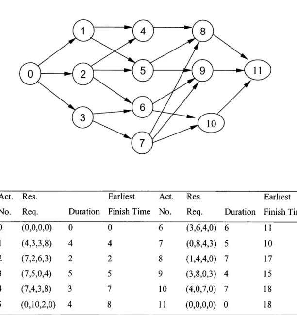
Act. No. Res. Req. Duration Earliest Finish Time Act. No. Res. Req. Duration Earliest Finish Time 0 (0,0,0,0) 0 0 6 (3,6,4,0) 6 11 1 (4,3,3,8) 4 4 7 (0,8,4,3) 5 10 2 (7,2,6,3) 2 2 8 (1,4,4,0) 7 17 3 (7,5,0,4) 5 5 9 (3,8,0,3) 4 15 4 (7,4,3,8) 3 7 10 (4,0,7,0) 7 18 5 (0,10,2,0) 4 8 11 (0,0,0,0) 0 18

Figure 3.3. Example test problem with scheduling results

A typical problem is illustrated in Figure 3.3. Precedence relationships between the activities are depicted on the activity-on-nodes (AON) network. Activities 0 and 11 are the dummy start and finish activity with duration 0, respectively. The durations of the other activities, number of units required by each activity and resource requirements are shown in the table below the network. There are four

(44)

different resource types. Resource availabilities are 27, 18, 25 and 22. Earliest finish times and the critical path duration are computed by perfonning CPM calculations in which the resource constraints are not considered. In this example, critical path is equal to 18. The absolute due date, T is set to 20.

CHAPTER 3. PROBLEM FORMULATION AND SOLUTION PROCEDURE 32

Iter. Activity 8 Activity 10 Activity 11

No

X8,17 X8.18 X8,I9 X8,20 X|0,I8 Xl0,19 Xl0,20 Xll,18 X||,I9 Xll,20

1 0 1 0 0 1 0 0 1 0 0 2 0 0 1 0 1 0 0 0 1 0 3 0 0 1 0 0 1 0 0 1 0 4 0 1 0 0 1 0 0 0 1 0 5 0 1 0 0 0 1 0 0 1 0 6 0 1 0 0 1 0 0 0 0 1 7 0 1 0 0 0 1 0 0 0 1 8 0 1 0 0 0 0 1 0 0 1 9 0 0 0 1 0 0 1 0 0 1

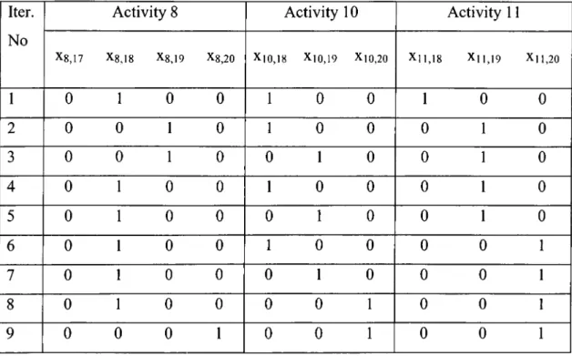
Table 3.3: The integer values of the selected variables as part of the MIP relaxation solution in each iteration

The IP model of this problem contains 220 variables 155 of which are previously set to 0 since these variables represent the activity finish times that are not between earliest and latest finish time periods. There are 11 activity completion, 18 precedence relationship and 80 resource constraints. We have 155 more constraints due to the variables set to 0. In order to decide which variables will be fixed to the integer values among the remaining 65 variables, we order the earliest finish times of the activities in the example and select activity 8, 10 and 11 that have the maximum earliest finish times. These activities have 10 active

(45)

variables, which are not set to 0. These 10 variables will be fixed to the corresponding integer values in the MIP relaxation optimal solution.

We relax the integrality constraints of variables except the fixed variables of activities 8, 10 and 11. The relaxed problem has a non-integral solution with the objective value 18. In table 3.3, in the first iteration the integral values of these variables, which are fixed, are shown. We put these values to the original problem; we obtain a subproblem, which does not explicitly contain the fixed variables of the activity 8, 10 and 11. We solve the problem with Cplex MIP version and it is found infeasible. Therefore, we add the following cut to the original problem:

- Xg,I7 + XS.18 - X8,I9 - X8,20 + Xl0,18 ' X|0,19 ‘ Xl0,20+ Xl 1,18'Xl 1,19 - Xll,20 ^ 2 (16)

When we resolve the relaxation of our original problem together with the new cut we added, the solution and the objective value change. The new objective value is 19. Therefore, lower bound increases by one and becomes 19. The integral values of the fixed variables as part of the MIP relaxation solution are shown in the second iteration on table 3.3. We fix these variables to their values and solve the subproblem. The subproblem is found infeasible. Therefore, we append one more cut to the original problem:

- X8,I7 -X8,18 + X8,I9 ‘ X8,20 + Xl0,18 ' Xl0,19 ’ Xl0,20- Xl 1,18 + Xl 1,19 - Xll,20^ 2 (17)

The relaxation of the original problem together with these two cuts is solved. The objective function stays the same in the third iteration. In the same manner, we generate the subproblem by fixing the values of the variables on the table, solve it, find the subproblem infeasible and generate a new cut. In this way, we added the following cuts until we reach the 6"’ iteration.

- X8,17 -X8,18 + X8,19 ' X8,20 ‘ Xl0,18 + Xl0,19 ' Xl0,20- Xl 1,18 + Xl 1,19 ‘ Xll,20 ^ 2 (18) - X8,17 + X8,18 - X8,19 " X8,20 + Xl0,18 ' Xl0,19 " Xl0,20- Xll,18 + Xll,19- Xll,20 ^ 2 (19)

(46)

-X8,I7+X8,I8 - X8,19 - X8,20-X|0,I8 +X|0,I9 * X|0,20 " Xl 1,18 + Xl 1,19 ‘ X| 1,20 ^ 2 (20)

In iteration 6, with the cuts added to the problem, the lower bound becomes 20. Therefore, the lower bound is improved by one.

In iteration 6,7 and 8, we obtain and add the following cuts respectively;

-X8,17 + X8,I8 - X8,19 " X8,20 + Xl0,18 " Xl0,19 ‘ Xl0,20 Xl 1,18 “Xl 1,19 + X| 1,20 ^ 2 (21) - Xg,|7 + X8,18 - X8,19 -X8,20-Xl0,18 + Xl0,19 ' Xl0,20 ' Xl 1,18 "Xl 1,19 +Xl 1,20 ^ 2 (22) - Xg,l7 + X8,18 - X8.19 - X8,20-Xl0,18 - Xl0,19 + Xl0,20 " Xl 1,18 ' Xl 1,19+Xl 1,20 ^ 2 (23)

CHAPTER 3. PROBLEM FORMULA TION AND SOL UTION PROCEDURE 34

In iteration 9, we find a feasible solution to the subproblem generated and thus a feasible solution to the original problem. The objective function of the solution is 20. Then we stop, since we find the optimal solution in which lower bound is equal to the upper bound. The optimal solution with schedule length of 20 is X|,4 = 1, X2,2 - 1, X3,5 = 1, X4,13~ 1, Xs,8 = 1, X6,ll ’ 1, X7,13 ~ 1, X8,20= 1,X9,20 = 1, X10,20 = 1, xii,2o = 1 with other variables that are found to be 0. The computational time needed to solve this problem is 0.46 CPU seconds.

(47)

3.4 Remarks

In this chapter, we presented the IP formulation of the problem and the two phased approximation algorithm. In the first phase, we tried to solve this problem, which contains a large number of constraints and variables. Since LP relaxation of the problem is too weak, we tried to add enumerativo cuts proposed in the first stage of the algorithm to the problem to tighten the formulation and to improve the lower bound. If we cannot find an upper bound, which will be equal to the optimal solution in the first stage, we continue with the second stage in which we make use of the enumerativo cuts and the lower bound obtained in the first stage. Here, the objective of the problem formulation is modified so as to minimize the finish time of the activity with the maximum earliest finish time in the set of immediately preceding activities of the dummy finish activity.

We think that the search may be extended to the other immediately preceding activities of the dummy finish activity. We observe that the cuts related with these activities and the dummy finish activity will be very useful to cut the search space. In addition, the cuts obtained from the lower bound found at the end of the second stage may be used with the cuts obtained before to solve the exact version of the problem. By doing this, we were able to solve some of the instances in at most two hours while Cplex could not even find a feasible upper bound in one week. Since the implementation time of the algorithm for a single instance is limited to 1 hour, we did not present the results with longer than one hour.

(48)

Chapter 4 Computational Results

In this chapter, we present some computational results of the algorithm proposed in Chapter 3. In seetion 4.1, the problem instances used to test the efficiency of the algorithm are described. In section 4.2, we discuss and analyze the eomputational results.

4.1 Test data

In order to evaluate the performanee of our algorithm, we used three benchmark data sets of Kolisch et. al. (1995) and Kolisch and Sprecher (1997), which can be downloaded from the project scheduling library (PSPLIB) site at the following address ; http://www.bwl.uni-kiel.de/Prod/psplib/.These benchmark data sets J30, J60 and J90 consist of RCPSP instances with 30,60 and 90 aetivities, respectively. To generate these test problems, Kolisch et. al. (1995) and Kolisch and Sprecher (1997) develop instanee generator PROGEN that produces problem instanees with controlled difficulty by utilizing previously defined eontrol parameters, i.e. projeet characteristics. The PROGEN allows generating instances with different number