Hub Location Problem with Allowed Routing between Nonhub Nodes

Hub Location Problem with Allowed Routing

between Nonhub Nodes

Ali I˙rfan Mahmutog˘ulları, Bahar Yetis Kara

In this study, we relax one of the general assumptions in the hub location literature by allowing routed flows between nonhub nodes. In hub networks, different flows are consoli-dated and routed via collection, interhub, and distribution arcs. Due to consolidation, some flows travel long paths despite closeness of their origin and destination. In this study, we allow direct flows by penalizing by a scalar factor of original cost of transshipment between these arcs. We present mathematical models for median, center, and set covering versions of the problem for single- and multi-allocation cases. We test the models with the CAB and TR data sets. We discuss the properties of established direct connections for different models by using another mathematical model where the number of direct flows is bounded and interpret the effect of changes in problem parameters.

Introduction

Hub facilities are consolidation and dissemination points in many-to-many flow network systems. Instead of serving each origin–destination (O–D) pair directly, transshipments are made via hubs. As a result of this consolidation, economies of scale arise in interhub transitions. Transportation cost (or time) is discounted by a factorα (0 ≤ α ≤ 1) between two hub nodes.

Hubs are widely used in different areas of industry, such as cargo delivery, passenger transportation, and telecommunication networks. The hub location problem is to find optimal locations of hub facilities and allocations of nonhub nodes to hub nodes over a network. O’Kelly (1986a, b) motivated different versions of the hub location problem and the problem is one of the most attractive areas of study in the transportation and logistics literature. O’Kelly (1987) proposed first mathematical model to minimize the total cost of transportation over a network where the number of hubs to be opened is p (later referred to as the p-hub median problem). Different studies have been conducted for the p-hub median problem, such as O’Kelly (1992), Campbell (1996), Ernst and Krishnamoorty (1996, 1998, 1999), Skorin-Kapov, Skorin-Kapov, and O’Kelly (1996), Ebery (2001), Boland et al. (2004), and Marin, Canovas, and Landete

Correspondence: Bahar Yetis Kara, Department of Industrial Engineering, Bilkent University, Bilkent, 06800 Ankara, Turkey

e-mail: [email protected]

(2006). Recent surveys (Campbell, Ernst, and Krishnamoorty 2002; Alumur and Kara 2008; Kara and Taner 2011) give a detailed history and synthesis of recent trends in the hub location literature.

Campbell (1994) proposed center and cover version of the problem. The p-hub center problem is to minimize the maximum travel distance between two nodes by locating p hub facilities on a network. Kara and Tansel (2000) and Meyer, Ernst, and Krishnamoorthy (2009) presented different integer models for the p-hub center problem. The hub covering problem is to minimize the required number of hubs to ensure that travel time between each node pair on the network is less than a prespecified covering radius. Kara and Tansel (2003), Ernst, Jiang, and Krishnamoorty (2005), and Wagner (2008) introduced different models for the hub covering problem.

Hub location problems can be divided into two mainstream allocation structures: single- and multi- allocation. In single-allocation models, each nonhub node is allocated to only a single hub. In the multi-allocation case, the flow originating from or destinated to a node can be transferred via different pairs of hubs.

Many studies in the hub location literature include three common assumptions due to Alumur and Kara (2008). The first assumes that the hub network is fully connected, that is, an arc exists between every pair of hubs. The second assumes that interhub transition is dis-counted by a factorα as a result of economies of scale. The third assumes that no direct flow is allowed between nonhub nodes. Studies exist in the literature where the first assumption is relaxed. O’Kelly and Miller (1994) introduced various hub network designs, including a sub-graph induced by hubs, which is incomplete. Nickel, Schobel, and Sonneborn (2001) dealt with a multi-allocation version of the problem, considering the costs of building hubs and hub arcs separately. Campbell, Ernst, and Krishnamoorty (2005a, b) proposed construction of a fixed number of hub links with reduced unit costs. Alumur, Kara, and Karasan (2009) defined incomplete versions of single-allocation p-hub median, hub location with fixed costs, hub covering, and p-hub center network design problems. The effect of the discount factor is also considered in different studies in the literature. Although most of the hub location studies focus on a constant discount factor for interhub transition, O’Kelly and Bryan (1998) consid-ered an increasing cost at a decreasing rate as flow increases. Horner and O’Kelly (2001) presented another cost function that requires a sufficient flow to discount interhub transition. Racunicam and Wynter (2005) presented a nonlinear concave cost function and economies of scale is generated for interhub and hub-to-node transitions. Aykin (1994, 1995) and Sasaki, Furuta, and Suzuki (2008) studied different types of flows between each origin–destination pairs. The different allocation strategies of nodes to hubs are investigated in Aykin (1994, 1995). In these studies, one-hub-stop, two-hub-stop, and direct services were considered and these service types were determined by the allocations of nodes. Mathematical models and algorithms were presented for these different service types in Aykin (1995) and capacity con-straints were relaxed in Aykin (1994). Sasaki, Furuta, and Suzuki (2008) proposed a location problem where customers may attend to facilities directly or via one transfer point. In this article, we propose flow-based models for p-hub median problems and mathematical models for center and cover versions of the hub problems that have not been studied in the existing literature.

Various different hub location problems were considered, including competitive aspects (Marianov, Serra, and ReVelle 1999; Eiselt and Marianov 2009), queueing systems (Marianov and Serra 2003), and uncertainty of problem parameters (Contreras, Cordeau, and Laporte 2011;

Alumur, Nickel & Saldanha da Gama 2012). The extensions such as capacitated network, thresholds, and flow-dependent cost functions were investigated by Bryan (1998).

Hub networks with direct flows can alleviate some drawbacks of consolidation in practice. Since flows are consolidated at hub nodes and transferred via hub links, some flows travel longer paths when compared to distance between their origin and destination. For some flows, routing without visiting any hub between nodes may be considered as a practical solution to decrease the cost due to this long travel of flow (for an example, see the Results for median models section). Moreover, center and cover versions of hub location problems are related to the traveling times of flows, for example, in cargo delivery applications, some thresholds should be satisfied as a target service levels (e.g., overnight delivery). By sending some flows directly from their origins to destinations, the maximum traveling times can be reduced or the number of hubs can be decreased to ensure feasibility. Also, in air transportation industry for some cargo requiring VIP service, leased aircrafts could be used as sending the flow directly for this pair of nodes.

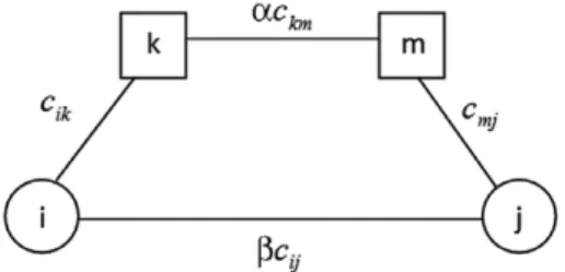
In this study, we relax one of the basic assumptions by allowing direct flow between two nonhub nodes. Fig. 1 explains the discount and penalty structure over the network for interhub and direct connections if nodes i and j are allocated to hubs k and m, respectively. cijis the unit travel time or cost between nodes i and j. Consider the flow from node i to node j. The flow can be routed via hubs with cost of cik+ αckm+ cmjper unit flow where the first term is collection, the second term is interhub transportation, and the third one is distribution cost. If routing between nonhub nodes is allowed, sending the flow over the link arc (i, j) becomes an alternative way to route the flow. However, establishing this direct flow will require some effort due to absence of consolidation and should be penalized to allow this direct flow in only extreme cases. Hence, we may assume that the cost of direct flow isβcijper unit flow whereβ ≥ 1. The cost of sending flow over arc (i, j) should be proportional to physical cost (which means thatβ ≥ 1) and the penalty of sending the flow directly bypassing the hub network.

The article is organized as follows: in the second, third, and fourth sections, we propose integer programming models for single- and multi-allocation cases of median, center, and hub covering models, respectively. In the fifth section, we present results of computational analysis of these models with CAB and TR data sets. The article ends with concluding remarks in the last section.

In the rest of the article, the fivefold taxonomy proposed by Kara and Taner (2011) is used to represent the problems. This taxonomy is in the form ofε/ϕ/κ/λ/ω, where these parameters represent objective criterion, allocation structure, capacity, interhub connectivity, and other restrictions, respectively. The parameter ε can be pH-median, pH-center and H-cover with respect to the minimum, minimax, and covering versions of the objective.ϕ is the allocation

structure of nonhub nodes. Either the single- or multi-allocation structure can be used for nonhub nodes. In the classical uncapacitated models,κ is U, λ is full, and ω entity is left blank.

p-hub median with allowed direct flow

Let G= (N, A) be a complete network, where N is the set of nodes {1, 2, . . . , n} and A is the set of arcs (i, j) such that i, j∈ N. The following parameters will be used in the models in the rest of the article:

p= number of hubs to be located, cij= length of arc (i, j) ∈ A,

wij= total flow originating from node i and destined to node j.

The classic p-hub median problem is to locate p hubs over the network and allocate nonhub nodes to hub nodes to minimize total cost of the traffic flow. In our model, there can be direct flows (not via hubs) between nodes. The maximum number of allowed direct transitions is q. Then, we define pH-median/single/U/full/direct and pH-median/multi/U/full/direct problems and present mathematical models for these problems in the following two subsections. Both models utilize multicommodity network flow variables similar to the ones presented in Ernst and Krishnamoorty (1998).

pH-median/single/U/full/direct problem

Let Oibe the total flow originating from node i, that is, Oi= ∑jwij. The decision variables used

in the model are as follows:

x if node i is allocated to hub j otherwise ij= ⎧⎨ ⎩ 1 0 , ,

y if direct connection is constructed between nodes i and j ot ij= 1 0 , , hherwise ⎧ ⎨ ⎩

fkmi =the amount of flow from hub k to hub m originating from node i gmj the amount of flow from hub m to node j originating from node i

i ₌

hik=the amount of flow from node i to hub k

Then, the mixed integer programming (MIP) model for pH-median/single/U/full/direct is as follows: min c hik ik c f c g w c y k i km km i m k i mj mj i j m i ij ij ij j i

∑

∑

∑

∑

∑

∑

∑

∑

∑

∑

∑

xkk p k

∑

∑

∑

∑

∑

∑

∑

∑

{ }

The first three terms in the objective value represent the collection, interhub transportation, and distribution costs, respectively. The last term stands for the cost of direct flow. Constraints (2) and (3) ensure that each node is allocated to a single hub facility. Constraint (4) guarantees that the number of hubs is p. Constraints (5) and (6) ensure the collection of nondirect (through hubs) flow from each node to its assigned hub. Similarly, constraints (7) and (8) are for the distribution. Constraint (9) is the flow balance equation. Constraint (10) allows consolidated flow between hub nodes only. Constraints (11) and (12) stand for non-negative and binary variables, respectively. pH-median/multi/U/full/direct problem

For the problem with multi-allocation, we additionally define xk, which takes the value of 1 if k is a hub node and 0 otherwise in this model. Because in the multi-allocation model a node can be allocated to more than one hub, a single-index variable xkis defined to identify whether node k was selected to be a hub or not. Definitions of parameters and other decision variables are the same as the single-allocation version of the model. The MIP for pH-median/multi/U/full/direct (multi-allocation p-hub median with allowed direct flows) is as follows:

min s t xk p k ( ) . . 1

∑

fkmi O x i k m i k

∑

Constraints (13), (14), (15), and (16) are similar versions of constraints (4), (6), (8), and (10), respectively. Constraint (4) is modified as constraint (13), which ensures the number of hubs to be open is p. Constraints (5), (7), and (9) adjust the flow balance based on whether a node is a hub or not.

p-hub center with allowed direct flow

The p-hub center problem is to minimize the maximum distance between pairs of nodes by locating p hubs and allocating nonhub nodes to hubs. In the following two subsections, we define single- and multi- allocation versions of the p-center problem with direct flows and present MIP models for these problems.

pH-center/single/U/full/direct problem

We define the decision variables xijand yijin similar manner as in the pH-median/single/U/full/ direct problem section. Let M= (2 + α)maxi,jcijbe a the maximum possible distance a flow can travel by using hubs. Value of M is obviously greater than travel disance of any flow and this fact is use to linearize the necesssary constraints. We also define Z as a free variable to keep the objective value of the model. Then, we can define MIP model for pH-center/single/U/full/direct as follows: min Z (18) s t Z cik ckm xik c x y M i j m k jm jm ij . . ≥

∑

The objective function (18) minimizes the maximum travel time between nodes whether via hubs or not. Constraints (19) and (20) define the distance between nodes i and j depending on the value of yij. If yij= 0, no flow from nonhub node i to nonhub node j is directly and the distance between these nodes is calculated based on the transition through hubs. Therefore, constraint (20) becomes redundant and constraint (19) stands for the distance between these two nodes. On the contrary, if yij = 1, constraint (19) becomes redundant since the LHS of the constraint gets negative value and the travel time of the direct flow is kept by constraint (20). Other constraints are used as in the previous models.

pH-center/multi/U/full/direct problem

In addition to the direct connection variable yij, we again must define the variables xk for hub nodes and Xijkmequals to 1 if flow from node i to node j is routed via hubs k and m in this order and 0 otherwise. As in the median case of multi-allocation,

min s t Z Xijkm cik ckm cmj y Mij i j m k ( ) . . ( ) 18 ≥

∑

∑

∑

∑

∑

∑

∑

∑

∑

∑

Constraints (20) and (21) correctly determine the distance between each pair of nodes. Regarding the value of yij, one of the constraints (20) and (21) become redundant. Constraint (22) ensures that each transition is made either via hubs or flow is sent directly and constraint (23) does not allow allocating a node to a nonhub node, where 2|N|3_x

kis the greatest value that the LHS of the constraint can take.

Hub set covering with allowed direct flow

The hub set-covering problem is to minimize the number of hubs to ensure that the length of the path between each pair of nodes is less than or equal to a predefined cover radius B. In the following two subsections, we define the H-cover/single/U/full/direct and H-cover/multi/U/full/ direct problems and present MIP models for these problems. As in the classic location literature, the models are similar to their center counterparts.

H-cover/single/U/full/direct problem The MIP model is as follows:

min xkk k

∑

The model minimizes the number of hubs (25). Constraints (26) and (27) together cor-rectly ensure that each pair of nodes is covered within the cover radius. If a direct connection is established between a pair of nodes, constraint (26) becomes redundant. On the contrary, if flow is sent directly, then constraint (27) gets redundant for corresponding node pair. Also, constraint (26) is valid for hubs to which nodes are allocated and redundant for other nonhub nodes and other hub facilities. Due to constraints (2) and (3), each node is allocated to exactly one hub.

H-cover/multi/U/full/direct problem

The MIP model for the H-cover/multi/U/full/direct problem can be presented as follows: min xk k

∑

∑

∑

Objective (28) minimizes the number of hubs to open. One of constraints (27) and (29) become redundant and the other one ensures that each pair of nodes is covered within the cover radius. Constraints (17), (22), and (23) are used in a similar manner as the model presented in the pH-center/multi/U/full/direct problem section.

Computational analysis

In this section, we present some computational results for the proposed models. We used the CAB data set presented by O’Kelly (1987) and TR data set presented by Tan and Kara (2007). All computational experiments are conducted on a 4× AMD Opteron Interlagos 16C 6282SE 2.6G 16M 6400MT PC running under LINUX. CPLEX version 12.4.0.0 was used to solve the models. Since the existence or absence of flow values in the objective has an impact on the results, the results will be discussed separately for median models (where flow values do appear in the objective function), and center and cover models (where flow values do not appear in the objective function).

Results for median models

Computational experiments for pH-median/single/U/full/direct and pH-median/multi/U/full/ direct problem on CAB data set, the instances are generated by varying the number of hubs p∈ {2, 3, 4, 5} and interhub discount factorα ∈ {0.2, 0.4, 0.6, 0.8}.

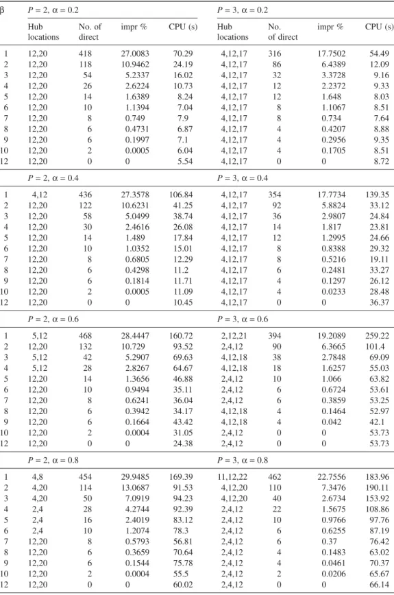
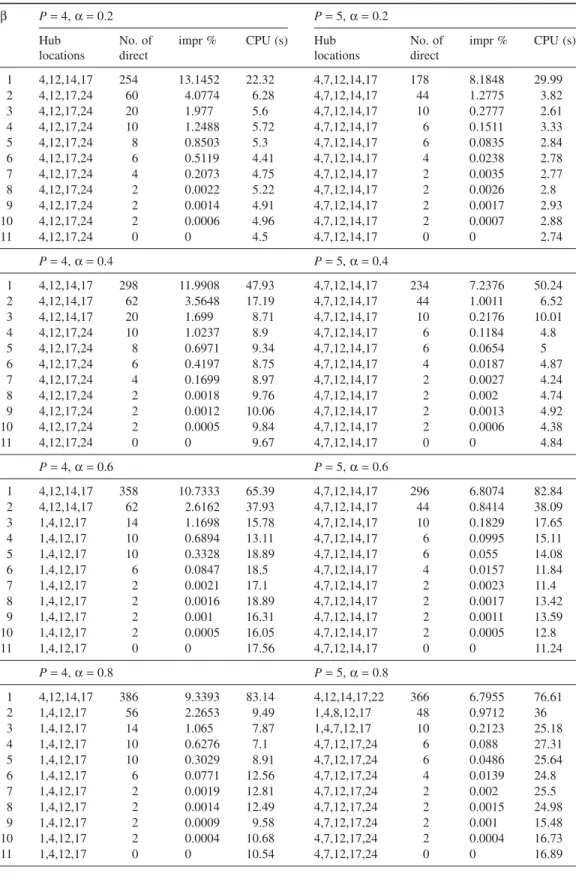
Tables 1–4 summarize the computational experimental results for pH-median/single/U/full/ direct and pH-median/multi/U/full/direct on CAB data set. For each parameter setting, that is, number of hubs to be opened (p), interhub discount factor (α), and direct flow penalty coefficient (β) following results are presented: hub locations, number of direct flows for the given parameter setting (no. of direct), decrease in the optimal objective value when compared to the optimal solution of classical problem where no direct flow is allowed (impr %), and CPU time required to solve the problem. Direct flow penalty coefficientβ is increased from 1 one-by-one up to 10 and in the last row for each p andα setting result for the minimum β value where no direct flow is sent.

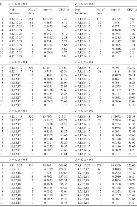
Sending flows directly from their origin to destination is more cost-efficient when discount factor α increases as a direct consequence of results. Moreover, when the number of hubs increases, a flow may benefit discounting more since there exists more hubs and discounted hub links in the network. When single- and multi-allocation strategies are compared, we observe that the number of direct flows is less than that in multi-allocation setting. This is a direct consequence of the possibility that a flow may possibly find a less costly path via hubs in multi-allocation setting.

Table 1 pH-Median/Single/U/Full/Direct Results on CAB Data Set with P= 2 and 3 β P= 2, α = 0.2 P= 3, α = 0.2 Hub locations No. of direct

impr % CPU (s) Hub

locations No. of direct impr % CPU (s) 1 12,20 418 27.0083 70.29 4,12,17 316 17.7502 54.49 2 12,20 118 10.9462 24.19 4,12,17 86 6.4389 12.09 3 12,20 54 5.2337 16.02 4,12,17 32 3.3728 9.16 4 12,20 26 2.6224 10.73 4,12,17 12 2.2372 9.33 5 12,20 14 1.6389 8.24 4,12,17 12 1.648 8.03 6 12,20 10 1.1394 7.04 4,12,17 8 1.1067 8.51 7 12,20 8 0.749 7.9 4,12,17 8 0.734 7.64 8 12,20 6 0.4731 6.87 4,12,17 4 0.4207 8.88 9 12,20 6 0.1997 7.1 4,12,17 4 0.2956 9.35 10 12,20 2 0.0005 6.04 4,12,17 4 0.1705 8.51 12 12,20 0 0 5.54 4,12,17 0 0 8.72 P= 2, α = 0.4 P= 3, α = 0.4 1 4,12 436 27.3578 106.84 4,12,17 354 17.7734 139.35 2 12,20 122 10.6231 41.25 4,12,17 92 5.8824 33.12 3 12,20 58 5.0499 38.74 4,12,17 36 2.9807 24.84 4 12,20 30 2.4616 26.08 4,12,17 14 1.817 23.81 5 12,20 14 1.489 17.84 4,12,17 12 1.2995 24.66 6 12,20 10 1.0352 15.01 4,12,17 8 0.8388 29.32 7 12,20 8 0.6805 12.29 4,12,17 8 0.5216 19.11 8 12,20 6 0.4298 11.2 4,12,17 6 0.2481 33.27 9 12,20 6 0.1814 11.71 4,12,17 4 0.1297 26.12 10 12,20 2 0.0005 11.09 4,12,17 4 0.0233 28.48 12 12,20 0 0 10.45 4,12,17 0 0 36.37 P= 2, α = 0.6 P= 3, α = 0.6 1 5,12 468 28.4447 160.72 2,12,21 394 19.2089 259.22 2 12,20 132 10.729 93.52 2,4,12 90 6.3665 101.4 3 5,12 42 5.2907 69.63 4,12,18 38 2.7848 69.09 4 5,12 28 2.8267 64.67 4,12,18 18 1.6257 55.03 5 12,20 14 1.3656 46.88 2,4,12 10 1.066 63.82 6 12,20 10 0.9494 35.11 2,4,12 6 0.6724 53.61 7 12,20 8 0.6241 36.04 2,4,12 6 0.3859 53.25 8 12,20 6 0.3942 34.17 4,12,18 4 0.1464 52.97 9 12,20 6 0.1664 43.42 4,12,18 4 0.042 42.1 10 12,20 2 0.0004 31.05 2,4,12 0 0 53.73 12 12,20 0 0 24.38 2,4,12 0 0 53.73 P= 2, α = 0.8 P= 3, α = 0.8 1 4,8 454 29.9485 169.39 11,12,22 462 22.7556 183.96 2 4,20 114 13.0687 91.53 4,12,20 110 7.3476 190.11 3 4,20 50 7.0919 94.23 4,12,20 40 2.6734 153.92 4 2,4 28 4.2744 92.39 2,4,12 22 1.5675 108.86 5 2,4 16 2.4019 83.12 2,4,12 10 0.9766 97.76 6 2,4 10 1.2074 78.3 2,4,12 6 0.6255 87.19 7 12,20 8 0.5793 56.81 2,4,12 6 0.37 76.42 8 12,20 6 0.3659 70.64 2,4,12 4 0.1483 63.02 9 12,20 6 0.1544 75.78 2,4,12 4 0.0461 70.37 10 12,20 2 0.0004 55.5 2,4,12 2 0.0206 65.67 12 12,20 0 0 60.02 2,4,12 0 0 66.14

Table 2 pH-Median/Single/U/Full/Direct Results on CAB Data Set with P= 4 and 5 β P= 4, α = 0.2 P= 5, α = 0.2 Hub locations No. of direct

impr % CPU (s) Hub locations No. of direct impr % CPU (s) 1 4,12,14,17 254 13.6724 17.22 4,7,12,14,17 178 8.7775 9.68 2 4,12,17,24 64 4.4687 8.17 4,7,12,14,17 52 1.6451 3.7 3 4,12,17,24 22 2.1455 6.66 4,7,12,14,17 12 0.3731 3.29 4 4,12,17,24 10 1.3404 7.16 4,7,12,14,17 6 0.1638 3.24 5 4,12,17,24 8 0.949 6.19 4,7,12,14,17 6 0.0973 3.22 6 4,12,17,24 6 0.6165 5.21 4,7,12,14,17 4 0.0385 3.28 7 4,12,17,24 6 0.314 6.72 4,7,12,14,17 4 0.0147 3.87 8 4,12,17,24 4 0.0214 5.65 4,7,12,14,17 2 0.0025 3.71 9 4,12,17,24 2 0.0014 5.67 4,7,12,14,17 2 0.0016 3.86 10 4,12,17,24 2 0.0006 6.72 4,7,12,14,17 2 0.0007 3.24 11 4,12,17,24 0 0 6.8 4,7,12,14,17 0 0 4.1 P= 4, α = 0.4 P= 5, α = 0.4 1 4,12,14,17 302 13.11 113.6 4,7,12,14,18 240 9.0961 102.47 2 4,12,14,17 78 3.715 62.34 4,7,12,14,17 58 1.818 44.88 3 1,4,12,17 22 1.4612 50.27 4,7,12,14,17 18 0.4059 26.11 4 1,4,12,17 12 0.8088 43.49 4,7,12,14,17 8 0.1691 16.74 5 1,4,12,17 10 0.398 25.04 4,7,12,14,17 6 0.098 16.25 6 1,4,12,17 6 0.1251 21.97 4,7,12,14,17 4 0.0533 14.2 7 1,4,12,17 4 0.0316 22.6 4,7,12,14,17 4 0.0352 11.2 8 1,4,12,17 4 0.0154 34.26 4,7,12,14,17 4 0.0171 13.08 9 1,4,12,17 2 0.0011 19.85 4,7,12,14,17 2 0.0012 10.69 10 1,4,12,17 2 0.0005 20.67 4,7,12,14,17 2 0.0006 13.09 11 1,4,12,17 0 0 17.16 4,7,12,14,17 0 0 12.72 P= 4, α = 0.6 P= 5, α = 0.6 1 4,12,14,18 350 13.9904 213.3 4,7,12,14,18 298 11.1672 228.38 2 1,4,12,17 82 3.9102 106.72 4,7,12,14,17 78 2.2964 122.64 3 1,4,12,17 26 1.5418 66.53 4,7,12,14,17 20 0.5724 97.35 4 1,4,12,17 12 0.7343 78.1 4,7,12,14,17 8 0.1968 78.28 5 1,4,12,17 10 0.3518 56.87 4,7,12,14,17 6 0.099 73.91 6 1,4,12,17 6 0.1229 53.46 4,7,12,14,17 4 0.0624 59.67 7 1,4,12,17 4 0.0446 48.41 4,7,12,14,17 4 0.0478 53.88 8 1,4,12,17 4 0.031 53.29 4,7,12,14,17 4 0.0332 55.97 9 1,4,12,17 4 0.0173 59.57 4,7,12,14,17 4 0.0186 58.67 10 1,4,12,17 4 0.0037 52.63 4,7,12,14,17 4 0.0039 58.23 11 1,4,12,17 0 0 54.81 4,7,12,14,17 0 0 64.7 P= 4, α = 0.8 P= 5, α = 0.8 1 8,11,12,22 420 18.362 206.07 7,8,11,12,22 378 14.8369 225.06 2 1,2,4,12 76 4.6329 174.3 1,4,6,12,17 68 3.1843 220.19 3 1,4,12,18 32 1.6251 130.83 1,4,7,12,18 26 0.7562 127.37 4 1,4,12,18 18 0.7908 137.36 1,4,7,12,18 14 0.2919 116.24 5 1,4,12,18 12 0.3973 102.31 1,4,7,12,18 10 0.1064 126.72 6 1,4,12,18 6 0.1868 96.35 1,4,7,12,18 4 0.0568 100.92 7 1,4,12,18 2 0.0425 99.29 1,4,7,12,18 2 0.0448 99.53 8 1,4,12,18 2 0.0312 93.64 1,4,7,12,18 2 0.0328 85.48 9 1,4,12,18 2 0.0199 88.78 1,4,7,12,18 2 0.0209 101.42 10 1,4,12,18 2 0.0085 85.33 1,4,7,12,18 2 0.009 81.85 11 1,4,12,18 0 0 85.45 1,4,7,12,18 0 0 114.8

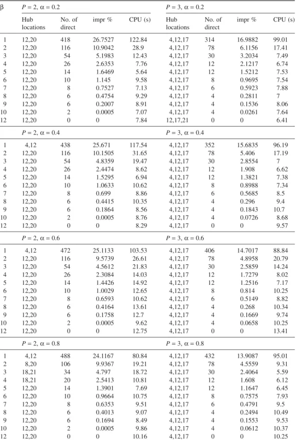
Table 3 pH-Median/Multi/U/Full/Direct Results on CAB Data Set with P= 2 and 3 β P= 2, α = 0.2 P= 3, α = 0.2 Hub locations No. of direct

impr % CPU (s) Hub

locations No. of direct impr % CPU (s) 1 12,20 418 26.7527 122.84 4,12,17 314 16.9882 99.01 2 12,20 116 10.9042 28.9 4,12,17 78 6.1156 17.41 3 12,20 54 5.1983 12.43 4,12,17 30 3.2034 7.49 4 12,20 26 2.6353 7.76 4,12,17 12 2.1217 6.74 5 12,20 14 1.6469 5.64 4,12,17 12 1.5212 7.53 6 12,20 10 1.145 9.58 4,12,17 8 0.9695 7.54 7 12,20 8 0.7527 7.13 4,12,17 6 0.5923 7.88 8 12,20 6 0.4754 9.29 4,12,17 4 0.2811 7 9 12,20 6 0.2007 8.91 4,12,17 4 0.1536 8.06 10 12,20 2 0.0005 7.07 4,12,17 4 0.0261 7.64 12 12,20 0 0 7.84 12,17,21 0 0 6.41 P= 2, α = 0.4 P= 3, α = 0.4 1 4,12 438 25.671 117.54 4,12,17 352 15.6835 96.19 2 12,20 116 10.1505 31.65 4,12,17 78 5.406 17.19 3 12,20 54 4.8359 19.47 4,12,17 30 2.8554 7 4 12,20 26 2.4474 8.62 4,12,17 12 1.908 6.62 5 12,20 14 1.5295 6.94 4,12,17 12 1.3821 7.38 6 12,20 10 1.0633 10.62 4,12,17 8 0.8988 7.34 7 12,20 8 0.699 8.86 4,12,17 6 0.5685 8.5 8 12,20 6 0.4415 10.35 4,12,17 4 0.296 9.4 9 12,20 6 0.1864 8.56 4,12,17 4 0.1843 10.7 10 12,20 2 0.0005 8.76 4,12,17 4 0.0726 8.68 12 12,20 0 0 8.29 4,12,17 0 0 9.57 P= 2, α = 0.6 P= 3, α = 0.6 1 4,12 472 25.1133 103.53 4,12,17 406 14.7017 88.84 2 12,20 116 9.5739 26.61 4,12,17 78 4.8958 20.79 3 12,20 54 4.5612 21.83 4,12,17 30 2.5859 14.24 4 12,20 26 2.3084 14.03 4,12,17 12 1.7279 8.02 5 12,20 14 1.4426 14.92 4,12,17 12 1.2516 7.17 6 12,20 10 1.0029 12.65 4,12,17 8 0.814 10.25 7 12,20 8 0.6593 10.62 4,12,17 6 0.5149 8.82 8 12,20 6 0.4164 13.61 4,12,17 4 0.268 10.34 9 12,20 6 0.1758 12.7 4,12,17 4 0.1669 9.74 10 12,20 2 0.0005 9.62 4,12,17 4 0.0658 10.25 12 12,20 0 0 12.75 4,12,17 0 0 13.41 P= 2, α = 0.8 P= 3, α = 0.8 1 4,12 488 24.1167 80.84 4,12,17 432 13.9087 95.01 2 8,20 106 9.9367 19.21 4,12,17 78 4.5559 9.31 3 18,21 34 4.797 18.72 4,12,17 30 2.4064 5.59 4 18,21 20 2.5413 10.81 4,12,17 12 1.608 6.12 5 12,20 14 1.3901 7.69 4,12,17 12 1.1647 6.45 6 12,20 10 0.9664 10.75 4,12,17 8 0.7575 7.93 7 12,20 8 0.6353 9.51 4,12,17 6 0.4791 9.5 8 12,20 6 0.4013 9.07 4,12,17 4 0.2494 10.49 9 12,20 6 0.1694 8.49 4,12,17 4 0.1553 9.53 10 12,20 2 0.0005 9.86 4,12,17 4 0.0612 10.37 12 12,20 0 0 10.16 4,12,17 0 0 10.25

Table 4 pH-Median/Multi/U/Full/Direct Results on CAB Data Set with P= 4 and 5 β P= 4, α = 0.2 P= 5, α = 0.2 Hub locations No. of direct

impr % CPU (s) Hub locations No. of direct impr % CPU (s) 1 4,12,14,17 254 13.1452 22.32 4,7,12,14,17 178 8.1848 29.99 2 4,12,17,24 60 4.0774 6.28 4,7,12,14,17 44 1.2775 3.82 3 4,12,17,24 20 1.977 5.6 4,7,12,14,17 10 0.2777 2.61 4 4,12,17,24 10 1.2488 5.72 4,7,12,14,17 6 0.1511 3.33 5 4,12,17,24 8 0.8503 5.3 4,7,12,14,17 6 0.0835 2.84 6 4,12,17,24 6 0.5119 4.41 4,7,12,14,17 4 0.0238 2.78 7 4,12,17,24 4 0.2073 4.75 4,7,12,14,17 2 0.0035 2.77 8 4,12,17,24 2 0.0022 5.22 4,7,12,14,17 2 0.0026 2.8 9 4,12,17,24 2 0.0014 4.91 4,7,12,14,17 2 0.0017 2.93 10 4,12,17,24 2 0.0006 4.96 4,7,12,14,17 2 0.0007 2.88 11 4,12,17,24 0 0 4.5 4,7,12,14,17 0 0 2.74 P= 4, α = 0.4 P= 5, α = 0.4 1 4,12,14,17 298 11.9908 47.93 4,7,12,14,17 234 7.2376 50.24 2 4,12,14,17 62 3.5648 17.19 4,7,12,14,17 44 1.0011 6.52 3 4,12,14,17 20 1.699 8.71 4,7,12,14,17 10 0.2176 10.01 4 4,12,17,24 10 1.0237 8.9 4,7,12,14,17 6 0.1184 4.8 5 4,12,17,24 8 0.6971 9.34 4,7,12,14,17 6 0.0654 5 6 4,12,17,24 6 0.4197 8.75 4,7,12,14,17 4 0.0187 4.87 7 4,12,17,24 4 0.1699 8.97 4,7,12,14,17 2 0.0027 4.24 8 4,12,17,24 2 0.0018 9.76 4,7,12,14,17 2 0.002 4.74 9 4,12,17,24 2 0.0012 10.06 4,7,12,14,17 2 0.0013 4.92 10 4,12,17,24 2 0.0005 9.84 4,7,12,14,17 2 0.0006 4.38 11 4,12,17,24 0 0 9.67 4,7,12,14,17 0 0 4.84 P= 4, α = 0.6 P= 5, α = 0.6 1 4,12,14,17 358 10.7333 65.39 4,7,12,14,17 296 6.8074 82.84 2 4,12,14,17 62 2.6162 37.93 4,7,12,14,17 44 0.8414 38.09 3 1,4,12,17 14 1.1698 15.78 4,7,12,14,17 10 0.1829 17.65 4 1,4,12,17 10 0.6894 13.11 4,7,12,14,17 6 0.0995 15.11 5 1,4,12,17 10 0.3328 18.89 4,7,12,14,17 6 0.055 14.08 6 1,4,12,17 6 0.0847 18.5 4,7,12,14,17 4 0.0157 11.84 7 1,4,12,17 2 0.0021 17.1 4,7,12,14,17 2 0.0023 11.4 8 1,4,12,17 2 0.0016 18.89 4,7,12,14,17 2 0.0017 13.42 9 1,4,12,17 2 0.001 16.31 4,7,12,14,17 2 0.0011 13.59 10 1,4,12,17 2 0.0005 16.05 4,7,12,14,17 2 0.0005 12.8 11 1,4,12,17 0 0 17.56 4,7,12,14,17 0 0 11.24 P= 4, α = 0.8 P= 5, α = 0.8 1 4,12,14,17 386 9.3393 83.14 4,12,14,17,22 366 6.7955 76.61 2 1,4,12,17 56 2.2653 9.49 1,4,8,12,17 48 0.9712 36 3 1,4,12,17 14 1.065 7.87 1,4,7,12,17 10 0.2123 25.18 4 1,4,12,17 10 0.6276 7.1 4,7,12,17,24 6 0.088 27.31 5 1,4,12,17 10 0.3029 8.91 4,7,12,17,24 6 0.0486 25.64 6 1,4,12,17 6 0.0771 12.56 4,7,12,17,24 4 0.0139 24.8 7 1,4,12,17 2 0.0019 12.81 4,7,12,17,24 2 0.002 25.5 8 1,4,12,17 2 0.0014 12.49 4,7,12,17,24 2 0.0015 24.98 9 1,4,12,17 2 0.0009 9.58 4,7,12,17,24 2 0.001 15.48 10 1,4,12,17 2 0.0004 10.68 4,7,12,17,24 2 0.0004 16.73 11 1,4,12,17 0 0 10.54 4,7,12,17,24 0 0 16.89

Another observation is the effect of direct links on the location of hubs. In many instances, allowing direct links changes the location of hubs. For example, in pH-median/single/U/full/ direct instance with p= 2 and α = 0.8, the hub sets when β = 1 and no direct flow is allowed are completely different.

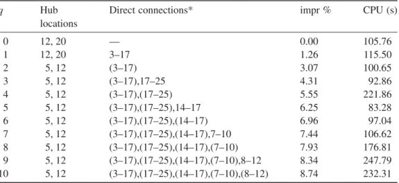
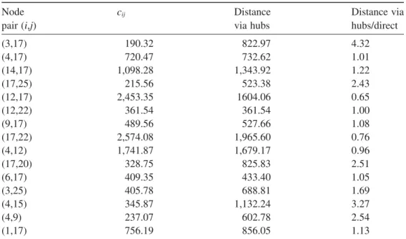
To observe the characteristics of direct flows, we conducted another analysis whereβ value is set to 1 and number of direct flows is bounded by a constant, q. Table 5 summarizes the results of this analysis for pH-median/single/U/full/direct with p= 2, α = 0.6 and q ∈ {1, . . . , 10}, and Table 6 presents the top 15 highest flow entity in CAB data set in decreasing order of flow with distance cij, distance via hubs values, and the ration between them. When both flows from 3 (Boston) to 17 (New York) and 17 to 3 are sent directly, the hub located at node 20 (Pittsburgh) is moved to the opposite direction and relocated at node 5 (Cincinnati). Fig. 2 depicts this situation. Sending some flows directly can be regarded as a decrease in the flow that should be carried via hub links in the corresponding area. Therefore, the locations of hubs are moved to the opposite direction to be able to get closer to the area where flow concentration is higher. By getting closer to the areas where flow values are greater, the cost of routing them via hubs decreases.

Also, for the node pair (3, 17), the optimal path via hubs is 3→ 20 → 17 and the resulting cost (882.97) is more than four times greater than the distance between these nodes (190.32) because they are both allocated to the same hub. In this case, then, direct flow between nodes 3 and 17 is preferable. The ratio of costs of sending one unit via hubs and directly is 4 32 822 97

190 32

. .

.

= for this pair of nodes. As this ratio increases, a flow is more likely to be sent directly rather than routed via hubs. This result can be verified from Tables 5 and 6 as well. Another observation from Table 5 is for odd values of q, the model chooses one node pair i and j, and flow from i to j is sent directly, whereas flow from j to i is routed via hubs.

Also, the flows are more likely to be sent directly since the objective is weighted average of cost of sending one unit of flow. We can see that this proposition holds true for flow from node 3 to node 17. The same situation does not apply to node pair 4 (Chicago) and 17, however, even though the flow between them is the second highest flow. Since the distance between them and Table 5 pH-Median/Single/U/Full/Direct Model for P= 2, α = 0.6 and β = 1 if the Number of Direct Flows is Bounded

q Hub

locations

Direct connections* impr % CPU (s)

0 12, 20 — 0.00 105.76 1 12, 20 3–17 1.26 115.50 2 5, 12 (3–17) 3.07 100.65 3 5, 12 (3–17),17–25 4.31 92.86 4 5, 12 (3–17),(17–25) 5.55 221.86 5 5, 12 (3–17),(17–25),14–17 6.25 83.28 6 5, 12 (3–17),(17–25),(14–17) 6.96 97.04 7 5, 12 (3–17),(17–25),(14–17),7–10 7.44 106.62 8 5, 12 (3–17),(17–25),(14–17),(7–10) 7.93 176.81 9 5, 12 (3–17),(17–25),(14–17),(7–10),8–12 8.34 247.79 10 5, 12 (3–17),(17–25),(14–17),(7–10),(8–12) 8.74 232.31

the traveling cost via hub is very close, sending the flow directly from 4 to 17 is not very profitable. Moreover, as q increases, hub set remains the same and marginal improvement in the objective decreases.

Another observation from Table 5 is for odd values of q, the model chooses one node pair i and j, and flow from i to j is sent directly, whereas flow from j to i is routed via hubs. Since the flow and cost values in CAB data set are symmetric, ties can be broken arbitrarily.

Our experiments also revealed that multi-allocation instances are solved in shorter CPU times even though the constraints that force single allocation in the pH-median/single/U/full/ direct model and the single-index hub variable are the only difference between the single- and multi-allocation models.

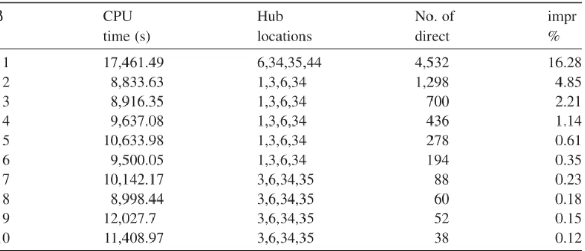
Since solution times of pH-median/single/U/full/direct are reasonable, we also observed the performance of the models on a larger data set. TR data set consisting of 81 nodes and 22 possible hub locations is used for the experiment. Table 7 presents some part of these experiment showing the required CPU time to solve pH-median/single/U/full/q-direct model on TR data set with Table 6 Top-15 Highest-Volume Flows in the CAB Data Set

Node pair (i,j) cij Distance via hubs Distance via hubs/direct (3,17) 190.32 822.97 4.32 (4,17) 720.47 732.62 1.01 (14,17) 1,098.28 1,343.92 1.22 (17,25) 215.56 523.38 2.43 (12,17) 2,453.35 1604.06 0.65 (12,22) 361.54 361.54 1.00 (9,17) 489.56 527.66 1.08 (17,22) 2,574.08 1,965.60 0.76 (4,12) 1,741.87 1,679.17 0.96 (17,20) 328.75 825.83 2.51 (6,17) 409.35 433.40 1.05 (3,25) 405.78 688.81 1.69 (4,15) 345.87 1,132.24 3.27 (4,9) 237.07 602.78 2.54 (1,17) 756.19 856.05 1.13

p= 4, α = 0.6, and β ∈ {1, . . . , 10}. We were able to solve the problem for a relatively great data set in a reasonable amount of time with and average of 10,756 s. As in CAB instances, allowing direct connection changes hub locations. However, node 6 (Ankara) and node 34 (Istanbul) have always been as hubs due to their geographical importance and density of flow. Since the network is large, the number of direct locations is much greater than CAB instances.

Results for center and cover models

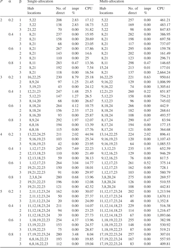
In Table 8, the results of computational experiments for center models are presented. As in the previous results for each parameter setting, hub locations decrease in the optimal objective value when compared to the optimal solution of classical problem where no direct flow is allowed (impr %), and CPU time required to solve the problem is presented. The first observation in center problems is the fact that the improvement in the objective is at most 8.79% and forβ value greater that or equal to 3, the optimal solution coincides with the optimal solution of the classical center models (impr % is 0%).

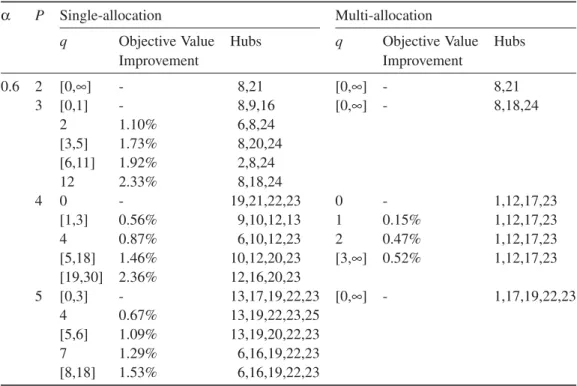
An important observation in these experiments is having alternative optimal solutions due to the fact that the objective is determined by one of the hub pairs and sending direct flow only for a small number of hub pairs can change the optimal solution. Then, the number of direct connections in Table 8 is misleading. Therefore, we conducted another analysis by fixing the β value to 1 and setting an upper bound on the number of direct flows where q is defined as number of allowed direct flow again. Table 9 presents the results for single- and multi-allocation center problems where β value is set to 1 and the number of direct connections is bounded by q.

In the center models, increasing the number of allowed direct flows does not always yield an improvement in the objective function value. We propose another mathematical model which is used to observe the points where the objective strictly improves as q increases. Assume that for a given value of q′, the problem is solved and the objective value of this problem turns out to be Z(q′). The following model can be used to find the next q value that the objective can improve in pH-center/single/U/full/direct problem:

Table 7 Solution Times of pH-Median/Single/U/Full/Direct on TR Data Set with P= 4 and α = 0.6 β CPU time (s) Hub locations No. of direct impr % 1 17,461.49 6,34,35,44 4,532 16.28 2 8,833.63 1,3,6,34 1,298 4.85 3 8,916.35 1,3,6,34 700 2.21 4 9,637.08 1,3,6,34 436 1.14 5 10,633.98 1,3,6,34 278 0.61 6 9,500.05 1,3,6,34 194 0.35 7 10,142.17 3,6,34,35 88 0.23 8 8,998.44 3,6,34,35 60 0.18 9 12,027.7 3,6,34,35 52 0.15 10 11,408.97 3,6,34,35 38 0.12

Table 8 pH-Center/Single/U/Full/Direct and pH-Center/Multi/U/Full/Direct Results on CAB Data Set P α β Single-allocation Multi-allocation Hub locations No. of direct impr % CPU Hub locations No. of direct impr % CPU 2 0.2 1 5,22 208 2.83 17.12 5,22 257 0.00 461.21 2 5,22 138 2.83 18.73 5,22 169 0.00 483.17 3 21,22 70 0.00 31.82 5,22 98 0.00 847.83 0.4 1 8,21 237 0.00 15.95 8,21 282 0.00 386.95 2 8,21 158 0.00 20.69 8,21 198 0.00 697.58 3 8,21 68 0.00 23.05 8,21 117 0.00 737.07 0.6 1 8,21 267 0.00 17.86 8,21 295 0.00 159.78 2 8,21 143 0.00 14.6 8,21 202 0.00 161.49 3 8,21 110 0.00 25 8,21 123 0.00 296.71 0.8 1 8,11 283 0.47 13.36 8,11 298 0.47 146.65 2 8,21 192 0.00 7.54 15,24 213 0.01 177.01 3 8,21 118 0.00 16.54 8,21 137 0.00 2,664.24 3 0.2 1 16,22,25 230 8.79 25.18 16,22,25 221 0.63 950.61 2 8,9,24 97 1.25 21.45 9,16,22 129 0.00 1,006.99 3 5,19,23 43 0.00 24.12 9,16,22 74 0.00 1,305.61 0.4 1 12,21,23 247 1.48 25.5 12,21,23 260 0.22 851.87 2 5,12,23 147 1.27 26.5 5,12,23 158 0.00 754.21 3 8,14,20 68 0.00 26.67 5,12,23 96 0.00 745.02 0.6 1 8,18,24 264 4.12 10.75 8,18,24 266 0.00 442.9 2 8,18,24 156 2.33 17.21 8,18,24 182 0.00 268.61 3 8,16,20 93 0.00 25.87 8,18,24 108 0.00 493.57 0.8 1 8,9,24 292 1.97 12.07 8,17,24 290 0.47 83.94 2 6,8,16 194 0.00 13.39 8,17,24 194 0.00 177.15 3 6,8,16 115 0.00 17.76 8,17,24 121 0.00 364.68 4 0.2 1 13,22,24,25 211 2.02 44.94 13,14,22,25 224 2.02 896.41 2 9,16,19,23 103 0.00 25.34 9,16,19,23 120 0.00 1,107.43 3 9,16,19,23 42 0.00 23.95 9,16,19,23 64 0.00 1,085.53 0.4 1 1,12,17,23 245 7.69 22.23 1,3,12,23 235 1.95 652.59 2 12,13,18,23 110 0.00 21.49 9,12,16,23 129 0.00 946.29 3 12,13,18,23 59 0.00 38.13 9,12,16,23 76 0.00 817.5 0.6 1 1,12,17,23 264 3.04 14.77 1,12,17,23 261 0.52 375.14 2 19,21,22,23 150 0.00 18.01 1,12,17,23 162 0.00 728.1 3 19,21,22,23 91 0.00 29.97 1,12,17,23 103 0.00 580.79 0.8 1 2,3,8,24 280 0.68 13.96 3,8,20,24 275 0.00 269.57 2 19,21,22,23 196 0.00 12.08 3,8,20,24 126 0.00 510.55 3 19,21,22,23 121 0.00 42.52 3,8,20,24 108 0.00 442.81 5 0.2 1 2,11,12,23,24 162 0.00 30.07 11,12,17,23,24 202 0.00 1,213.94 2 2,11,12,23,24 50 0.00 27.37 11,12,17,23,24 87 0.00 1,670.11 3 2,11,12,23,24 20 0.00 24.09 11,12,17,23,24 48 0.00 1,352.8 0.4 1 11,12,18,23,24 211 0.00 14.07 11,12,14,18,23 229 0.00 516.38 2 11,12,18,23,24 94 0.00 23.25 11,12,14,18,23 114 0.00 1,216.47 3 11,12,18,23,24 39 0.00 27.73 11,12,14,18,23 67 0.00 1,093.66 0.6 1 1,18,19,22,23 254 4.37 13.96 1,18,19,22,23 255 0.00 382.98 2 13,19,22,23 153 0.00 24.57 1,18,19,22,23 148 0.00 530.92 3 13,19,22,23 75 0.00 28.87 1,18,19,22,23 87 0.00 519.21 0.8 1 17,19,22,23,24 280 3.48 8.04 17,19,22,23,24 257 0.00 307.01 2 6,8,16,22,23 193 0.00 19.85 17,19,22,23,24 167 0.00 557.93 3 6,8,16,22,23 112 0.00 19.04 17,19,22,23,24 83 0.00 409.81

min q (30) s t. . Z q( )′ − ≥ εZ (31) yij q i j<

∑

The optimal value of objective (30) represents the next q value with q> q′ that improves the objective of the problem. Constraint (31) ensures that the decrease in the objective allows for small enough values ofε > 0. Constraint (31) limits the number of direct flows. Constraints (2), (3), (4), (12), (19) and (20) were used as defined in the previous sections. We use a similar model to determine the improvement step points for the multi-allocation version of the problem.

Despite the median version of the model in the center problems, direct flow is between distant origin–destination pairs. Our computational studies reveal that in center models, the hubs are located farther apart when the allowed number of direct connections increases. The reason behind this result is because more discount can be achieved by distant hubs. Direct flows are routed to compensate for the increase in the objective that arises from of hubs farther apart.

Another important point is in multi-allocation center problem; we cannot achieve so much improvement since multi-allocation already gives us the opportunity to route the flows over different hub links.

Table 9 pH-Center/Single/U/Full/Direct and pH-Center/Multi/U/Full/Direct Models forα = 0.6 if the Number of Direct Flows is Bounded

α P Single-allocation Multi-allocation

q Objective Value Improvement

Hubs q Objective Value

Improvement Hubs 0.6 2 [0,∞] - 8,21 [0,∞] - 8,21 3 [0,1] - 8,9,16 [0,∞] - 8,18,24 2 1.10% 6,8,24 [3,5] 1.73% 8,20,24 [6,11] 1.92% 2,8,24 12 2.33% 8,18,24 4 0 - 19,21,22,23 0 - 1,12,17,23 [1,3] 0.56% 9,10,12,13 1 0.15% 1,12,17,23 4 0.87% 6,10,12,23 2 0.47% 1,12,17,23 [5,18] 1.46% 10,12,20,23 [3,∞] 0.52% 1,12,17,23 [19,30] 2.36% 12,16,20,23 5 [0,3] - 13,17,19,22,23 [0,∞] - 1,17,19,22,23 4 0.67% 13,19,22,23,25 [5,6] 1.09% 13,19,20,22,23 7 1.29% 6,16,19,22,23 [8,18] 1.53% 6,16,19,22,23

In Table 10, hub locations, optimal objective value (number of hubs to be opened), and required CPU times results of our computational experiments for the H-cover/single/U/full/direct and H-cover/multi/U/full/direct problems are presented. The experiments are conducted forα = 0.6 and 0.8 since for these values, cover radii are available in Kara and Tansel (2003). As previously observed in center models, direct flows are sent between distant O–D pairs in cover models. Also, due to the structure of cover type objective, the problem can be solved within seconds for all instances.

Table 11 presents the outputs in the bounded number of direct flows forα = 0.8 since in cover problem, there exist alternative optima and the number of direct flows is larger unless it is bounded. The instance with andβ = 2,307 is noteworthy since we require 22 direct flows in order to decrease the objective by one. On the contrary, allowing routing between nonhub pairs does not yield significant improvements in the multi-allocation case, wherein only one of the instances the objective improves as q increases (α = 0.8 and β = 2,713). In other instances, no improvement is observed.

Center and cover models are also tested with TR data set. However, the models that require four-index variables or constraints with four dimension cannot be solvable due to memory Table 10 H-Cover/Single/U/Full/Direct and H-Cover/Multi/U/Full/Direct Results on CAB Data Set

α B β Single-allocation Multi-allocation

Hub locations Objective CPU Hub locations Objective CPU

0.6 2557 1 22,23,25 3 0.24 22,23,25 3 0.18 2 8,13,25 3 1.04 8,21,23 3 0.86 3 7,8,25 3 1.3 1,5,8 3 0.86 2336 1 2,8,24 3 0.29 2,8,24 3 0.25 2 8,14,18 3 0.82 8,18,24 3 0.74 3 8,9,18,24 4 1.2 5,8,18,24 4 1.15 2184 1 12,18,23,24 4 0.32 1,2,12,23 4 0.24 2 19,21,22,23 4 0.8 19,21,22,23 4 0.87 3 19,21,22,23 4 1.21 19,21,22,23 4 0.88 2002 1 6,14,19,22,23 5 0.34 19,20,22,23,24 5 0.31 2 1,19,21,22,23,25 6 0.72 1,19,21,22,23,25 6 0.58 3 6,11,13,19,22,23 6 1.21 8,9,12,16,22,23 6 0.84 0.8 2713 1 15,23 2 0.24 15,23 2 0.15 2 8,11,23 3 0.75 8,11,23 3 0.61 3 5,8,11 3 0.99 8,21,23 3 0.7 2552 1 8,14,25 3 0.38 6,8,14 3 0.16 2 4,8,13,23 4 0.83 2,3,11,14 4 0.61 3 19,21,22,23 4 0.99 8,13,17,23 4 0.73 2457 1 8,14,17,23 4 0.32 3,8,24,25 4 0.41 2 12,21,22,23 4 0.75 12,21,22,23 4 0.59 3 19,21,22,23 4 0.98 19,21,22,23 4 0.74 2307 1 6,12,22,23,24 5 0.28 6,12,22,23,24 5 0.2 2 11,18,19,22,23,24 6 0.58 11,18,19,22,23,24 6 0.6 3 7,19,20,22,23,24 6 0.98 11,17,19,22,23,24 6 0.75

requirement. Thus, only pH-center/single/U/full/direct problem can be solved for TR data set. Table 12 presents the results for TR instances with p= 4 and α = 0.6 for this problem.

All computational experiments showed that when the model constraints becomes stronger such as when the number of hubs to be located is small and each node is allocated to only one hub, better improvements in objective values can be made by allowing direct flow between nonhub nodes.Transferring via hubs is quite economical when multi-allocation is allowed. When compared to the direct connection cost, especially for small values ofα and great values of β, hubbing is a cheaper way to connect O–D pairs.

To deal with larger data sets, some heuristic approaches may be developed. Many heuristic approaches can be adopted for the case where routing between nonhub nodes is allowed. As pointed in Aykin (1995), if hub locations are given, pH-median/multi/U/full/direct problem decomposes in subproblems for each pair of nodes. Therefore, a promising selection with a heuristic approach would give a near-optimal solution. Moreover, as in TA_A and TA_B heuristic in Chen (2013), some heuristics can be improved that first selects hub nodes, then give allocation decision and finally determine routes between nonhub nodes.

An interested reader may find maps and detailed information about CAB and TR data sets in O’Kelly (1987) and Tan and Kara (2007), respectively.

Conclusion

In this study, we relaxed one of the common assumptions in the hub location literature by allowing traffic flow between nonhub nodes. We present mathematical models and discuss Table 11 H-Cover/Single/U/Full/Direct and H-Cover/Multi/U/Full/Direct Models forα = 0.8 if the Number of Direct Flows is Bounded

α B Single-allocation Multi-allocation

q Objective Hub locations q Objective Hub locations

0.8 2713 0 3 11,12,23 0 3 4,8,11 [1,∞] 2 8,11 [1,∞] 2 8,11 2552 [0,1] 4 4,8,13,23 [0,∞] 3 8,14,17 [2,∞] 3 4,8,24 2457 [0,∞] 4 19,21,22,23 [0,∞] 4 8,15,17,24 2307 [0,21] 6 9,11,12,22,23,24 [0,∞] 5 17,19,22,23,24 [22,∞] 5 9,12,22,23,24

Table 12 Solution Times of pH-Center/Single/U/Full/Direct on TR Data Set with P= 4 and α = 0.6

β CPU time (s) Hub locations No. of

direct impr % 1 2,081.02 3,25,34,65 2,955 1.71 2 26,195.2 3,5,21,34 1,663 0.92 3 33,082.16 21,25,34,68 393 0.00 4 19,837.34 21,25,34,68 191 0.00 5 49,916.32 21,25,34,68 87 0.00

median, center, and cover objectives under single- and multi-allocation strategies. Hub networks benefit from economies of scale generated from consolidation and a decreased number of established links. However, in some cases, allowing direct flow between nonhub nodes may result in improved objectives. Allowing a direct flow between with a cost penalty, O–D pairs may change allocations and even the locations of hubs on the network.

We conducted computational experiments to observe the solutions where direct flow is penalized and deduce the properties of candidate locations for direct flows where the number of direct flows is bounded. For median-objective models, the amount of flow and the allocation decisions affect the direct flow decisions. On the contrary, in center- and cover-objective models, direct flow decisions are made based on the distances and the allocation structure.

As a future research direction, there can be some extensions of the problem. For example, instead of sending all flows from one to another, one can consider the case where some portion of the flow is sent directly. Also, direct flow decisions are highly dependent on the interhub discount factor. Another interesting research would be the case where interhub cost decreases as the flow increases, as in O’Kelly and Bryan (1998).

References

Alumur, S., and B. Y. Kara. (2008). “Network Hub Location Problems: The State of the Art.” European Journal of Operational Research 190(1), 1–21.

Alumur, S., S. Nickel, and F. Saldanha da Gama. (2012). “Hub Location under Uncertainty.” Transpor-tation Research Part B: Methodological 46(4), 529–43.

Alumur, S. A., B. Y. Kara, and O. E. Karasan. (2009). “The Design of Single Allocation Incomplete Hub Networks.” Transportation Research Part B: Methodological 40(10), 936–51.

Aykin, T. (1994). “Lagrangian Relaxation Based Approaches to Capacitated Hub-and-Spoke Network Design Problem.” European Journal of Operational Research 79(3), 501–23.

Aykin, T. (1995). “Networking Policies for Hub-and-Spoke Systems with Application to the Air Trans-portation System.” TransTrans-portation Science 29(3), 201–21.

Boland, N., M. Krishnamoorty, A. T. Ernst, and J. Ebery. (2004). “Preprocessing and Cutting for Mul-tiple Allocation Hub Location Problems.” European Journal of Operational Research 155(3), 638–53.

Bryan, D. (1998). “Extensions to the Hub Location Problem: Formulations and Numerical Examples.” Geographical Analysis 30(4), 315–30.

Campbell, J. F. (1994). “Integer Programming Formulations of Discrete Hub Location Problems.” Euro-pean Journal of Operational Research 72, 387–405.

Campbell, J. F. (1996). “Hub Location and P-Hub Median Problem.” Operations Research 44(6), 1–13. Campbell, J. F., A. T. Ernst, and M. Krishnamoorty. (2002). “Hub Location Problems.” In Facility

Loca-tions Application and Theory, 373–407, edited by Z. Drezner and H. W. Hamacher. Berlin: Springer.

Campbell, J. F., A. T. Ernst, and M. Krishnamoorty. (2005a). “Hub Arc Location Problems: Part I—Introduction and Results.” Management Science 51(10), 1540–55.

Campbell, J. F., A. T. Ernst, and M. Krishnamoorty. (2005b). “Hub Arc Location Problems: Part II—Formulations and Optimal Algorithms.” Management Science 51(10), 1556–71.

Chen, J. (2013). “Heuristics for Hub Location Problems with Alternative Capacity Levels and Allocation Constraints.” In Intelligent Computing Theories, 207–16, edited by D.-S. Huang, V. Bevilacqua, J. C. Figueroa, and P. Premaratne. Nanning: Springer.

Contreras, I., J. Cordeau, and G. Laporte. (2011). “Stochastic Uncapacitated Hub Location.” European Journal of Operational Research 212(3), 518–28.

Ebery, J. (2001). “Solving Large Single Allocation P-Hub Problems with Two or Three Hubs.” European Journal of Operational Research 128(2), 447–58.

Eiselt, H. A., and V. Marianov. (2009). “A Conditional P-Hub Location Problem with Attraction Func-tions.” Computers and Operations Research 36(12), 3128–35.

Ernst, A. T., and M. Krishnamoorty. (1996). “Efficient Algorithms for the Uncapacitated Multiple Allo-cation P-Hub Median Problem.” LoAllo-cation Science 4(3), 139–54.

Ernst, A. T., and M. Krishnamoorty. (1998). “Exact and Heuristic Algorithms for the Uncapacitated Multiple Allocation P-Hub Median Problem.” European Journal of Operational Research 104, 100–12.

Ernst, A. T., and M. Krishnamoorty. (1999). “Solution Algorithms for the Capacitated Single Allocation Hub Median Problem.” Annals of Operations Research 86, 141–59.

Ernst, A. T., H. Jiang, and M. Krishnamoorty. (2005). Reformulations and Computational Results for Uncapacitated Single and Multiple Allocation Hub Covering Problems. Clayton South Vic: CSIRO Mathematical and Information Sciences.

Horner, M. W., and M. E. O’Kelly. (2001). “Embedding Economies of Scale Concepts for Hub Network Design.” Journal of Transport Geography 9(4), 255–65.

Kara, B. Y., and M. R. Taner. (2011). “Hub Location Problems: The Location of Interacting Facilities.” In Foundations of Location Analysis, 273–88, edited by H. A. Eiselt and V. Marianov. London: Springer.

Kara, B. Y., and B. C. Tansel. (2000). “On the Single Assignment P-Hub Center Problem.” European Journal of Operational Research 125, 648–55.

Kara, B. Y., and B. C. Tansel. (2003). “The Single-Assignment Hub Covering Problem: Models and Lin-earizations.” Journal of the Operational Research Society 54, 59–64.

Marianov, V., and D. Serra. (2003). “Location Models for Airline Hubs Behaving as m/d/c Queues.” Computers & Operations Research 30(7), 983–1003.

Marianov, V., D. Serra, and C. ReVelle. (1999). “Location of Hubs in a Competitive Environment.” European Journal of Operational Research 114(2), 363–71.

Marin, A., L. Canovas, and M. Landete. (2006). “New Formulations for the Uncapacitated Multiple Allocation Hob Location Problem.” European Journal of Operational Research 172(1), 274–92. Meyer, T., A. T. Ernst, and M. Krishnamoorthy. (2009). “A 2-Phase Algorithm for Solving the Single

Allocation P-Hub Center Problem.” Computers & Operations Research 36(12), 3143–51. Nickel, S., A. Schobel, and T. Sonneborn. (2001). Hub Location Problems in Urban Traffic Networks.

Boston: Kluwer Academic Publishers.

O’Kelly, M. E. (1986a). “Activity Levels at Hub Facilities in Interacting Networks.” Geographical Analysis 18(4), 343–56.

O’Kelly, M. E. (1986b). “The Location of Interacting Hub Facilities.” Transportation Science 20(2), 92–105.

O’Kelly, M. E. (1987). “A Quadratic Integer Program for the Location of Interacting Hub Facilities.” European Journal of Operational Research 32, 393–404.

O’Kelly, M. E. (1992). “Hub Facility Location with Fixed Costs.” Papers in Regional Science 71(3), 293–306.

O’Kelly, M. E., and D. L. Bryan. (1998). “Hub Location with Flow Economies of Scale.” Transportation Research Part B 32(8), 605–16.

O’Kelly, M. E., and H. J. Miller. (1994). “The Hub Network Design Problem—A Review and Synthe-sis.” Journal of Transport Geography 2(1), 31–40.

Racunicam, I., and L. Wynter. (2005). “Optimal Locations of Intermodel Freight Hubs.” Transportation Research Part B 39(5), 453–77.

Sasaki, M., T. Furuta & A. Suzuki. (2008). Exact optimal solutions of the minisum facility and transfer points location problems on a network. International Transactions in Operational Research 15(3), 295–306.

Skorin-Kapov, D., J. Skorin-Kapov, and M. O’Kelly. (1996). “Tight Linear Programming Relaxations of Uncapacitated P-Hub Median Problems.” European Journal of Operational Research 94, 582–93. Tan, P. Z., and B. Y. Kara. (2007). “A Hub Covering Model for Cargo Delivery Systems.” Networks

49(1), 28–39.

Wagner, B. (2008). “Model Formulations for Hub Covering Problems.” Journal of the Operational Research Society 59(7), 932–8.