Investigation of Hourly and Daily Patterns for
Lithosphere-Ionosphere Coupling Before Strong
Earthquakes
Seçil KARATAY1, Feza ARIKAN2, Orhan ARIKAN3
1Fırat University, Department of Physics, [email protected] 23100, Elazığ, Turkey
2Hacettepe University, Department of Electrical and Electronics, [email protected] 06800, Beytepe, Ankara, Turkey
3 Bilkent University, Department of Electrical and Electronics Engineering, [email protected] 06800, Bilkent, Ankara, Turkey
Abstract—The ionosphere can be characterized with its electron density distribution which is a complex function of spatial and temporal variations, geomagnetic, solar and seismic activity. An important measurable quantity about the electron density is the Total Electron Content (TEC) which is proportional to the total number of electrons on a line crossing the atmosphere. TEC measurements enable monitoring variations in the space weather. Global Positioning System (GPS) and the network of world-wide receivers provide a cost-effective solution in estimating TEC over a significant proportion of global land mass. In this study, five earthquakes between 2003–2008 that occurred in Japan with different seismic properties, and the China earthquake in May 2008 are investigated. The TEC data set is investigated by using the Kullback-Leibler Divergence (KLI), Kullback-Leibler Distance (KLD) and L2-Norm (L2N) which are used for the first time in the literature in this context and Cross Correlation Function (CCF) which is used in the literature before for quiet day period (QDP), disturbed day period (DDP), periods of 15 days before a strong earthquake (BE) and after the earthquake (AE). In summary, it is observed that the CCF, KLD and L2N between the neighbouring GPS stations cannot be used as a definitive earthquake precursor due to the complicated nature of earthquakes and various uncontrolled parameters that effect the behavior of TEC such as distance to the earthquake epicenter, distance between the stations, depth of the earthquake, strength of the earthquake and tectonic structure of the earthquake. KLD, KLI and L2N are used for the first time in literature for the investigation of earthquake precursor for the first time in literature and the extensive study results indicate that for more reliable estimates further space-time TEC analysis is necessary over a denser GPS network in the earthquake zones.
Keywords-component; Ionosphere, Total Electron Content, Kullback-Leibler, L2-Norm, Earthquke, Coupling
I. INTRODUCTION
Earth’s ionosphere is a dominant factor in space weather and the variability of the ionosphere is important for the ionospheric physics and radio communications. The ionosphere can be characterized with its electron density distribution which is a complex function of spatial and temporal variations, geomagnetic, solar and seismic activity. An important measurable quantity about the electron density is the Total Electron Content (TEC) which is proportional to the total number of electrons on a line crossing the atmosphere. The unit of TEC is given in TECU where 1 TECU = 1016el/m2. TEC measurements enable monitoring variations in the space weather. Global Positioning System (GPS) and the network of world-wide receivers provide a cost-effective solution in estimating TEC over a significant proportion of global land mass [1].
Recent studies in the literature indicate that there is a possible coupling between lithosphere and ionosphere before strong earthquakes [2-5]. In these studies, it is suggested that seismic activity causes several disturbances and variations in the ionosphere especially in the frequency and electron and ion compositions. To investigate this interaction, different statistical and physical models have been presented by using some parameters like electron density, Total Electron Content and critical frequency of F2-Layer. In the literature, the statistical tools that are used to investigate the effect of presismic activity on the ionosphere can be grouped into Correlation Analysis [3,4], Inter Quartile Range Analysis [6,7], TEC Difference Analysis [8] and Ionospheric Correction [8,9]. Among these studies, the most dominant and successful to provide pre-earthquake information is shown to be Correlation Analysis.
Kullback-Leibler Divergence (KLI), Kullback-Leibler Distance (KLD) [10,11] and L2-Norm (L2N) [12] are used in various description to define the similarity and the difference between two distributions. In this study, the Cross-Correlation Coefficient (CCF), KLI, KLD and the L2N are applied to TEC data for detailed investigation of lithosphere-ionosphere coupling. KLI, KLD and the L2N are used for the first time in the literature in this context. In addition, sliding window statistical properties of TEC are observed using moving average and standard deviation. In this study, five earthquakes between 2003–2008 that occurred in Japan with different seismic properties, and the China earthquake in May 2008 are chosen. TEC values are estimated for periods of 15 days before a strong earthquake (BE) and after the earthquake (AE) with a time resolution of 2.5 minutes and for all the GPS stations positioned near and far from the earthquake epicenter. TEC values are also obtained for the same GPS station group and with the same time resolution for the days when Ionosphere is under the influence of strong disturbances (disturbed day period-DDP) and also for the periods when there are no significant disturbances, geomagnetic storm or seismic activity in the regions (quiet day period-QDP). The statistical method used in the study and the results on the data are summarized in Section 2 and Section 3 respectively.
II. DESCRIPTIONOFTHEMETHOD
Vertical Total Electron Content (VTEC) is the sum of the free electrons estimated in the direction of the local zenith angle of the GPS receiver location. Let
[
(N)]
T d u; x (n)... d u; x (1)... d u; x d u; = x (1)represent the set of VTEC data of length N estimated for day of the d. Here, u indicates the receiver, n is the sample number (1≤ n ≤ N) and T is transpose of the operator.
In order to compare the behavior of TEC for the QDP period with those from the DDP, BE and AE periods, an average quiet day TEC estimate (AQDT) for each GPS station is obtained. From the overall amount of Nd days of uth station, AQDT is defined as:
∑
= = − s d i d n d n d u; d s d i d u; N1 x x (2)where di is the initial day and ds is the final day of QDP. To eliminate the seasonal and annual effects, the data vectors are normalized. For the day d, the experimental Probability Density Function (PDF), s d i d u; ˆ − P of the s d i d u; −
x
vector, can be approximated as follows: 1 s N i N n s d i u;d s d i u;d s d i u;d (n) ˆ x − = − − − ⎟⎟ ⎟ ⎟ ⎠ ⎞ ⎜⎜ ⎜ ⎜ ⎝ ⎛ = x∑
P (3)where Ni is the initial sample and Ns is the final sample Using this approximation described in Equation 3, the Kullback-Leibler Divergence KLI is defined as:
∑
∑
= − − − = − = − ⎟ ⎟ ⎠ ⎞ ⎜ ⎜ ⎝ ⎛ ⎟ ⎟ ⎠ ⎞ ⎜ ⎜ ⎝ ⎛ = s N i N n Pˆu;d(n) (n) s d i d u; Pˆ (n)ln s d i d u; Pˆ ) d u; ˆ s d i d u; ˆ KLI s N i N n Pˆu;di ds(n) (n) d u; Pˆ (n)ln d u; Pˆ ) s d i d u; ˆ d u; ˆ KLI P \ \ P ( P \ \ P ( (4)From the Equation 4, the symmetric Kullback-Leibler Distance KLD can be defined as follows [10,11-15]:
) d u; ˆ \ \ s d i d u; ˆ ( KLI ) s d i d u; ˆ \ \ d u; ˆ ( KLI ) s d i d u; ˆ ; d u; ˆ KLD(P P − = P P − + P − P (5)
For the energy normalized TEC distribution, the L2-Norm can be given as [12]: 2 s N i N n (n) s d i d u; Pˆ (n) d u; Pˆ ) s d i d u; ˆ d u; ˆ L2N
∑
= ⎟ ⎠ ⎞ ⎜ ⎝ ⎛ − = − -P \ \ P ( (6)The cross correlation coefficients (CCF) are determined by an correlation function as:
⎟ ⎠ ⎞ ⎜ ⎝ ⎛ − = ⎟ ⎠ ⎞ ⎜ ⎝ ⎛ = − − − −
∑
u;di ds u;di ds s i d u; d u; s d i d u; d u; T s d i d d, ; u Pˆ (n) ˆ N N n ˆ -(n) Pˆ N 1 σ σ r P P (7) where ˆPu ;d and s d i d ; u ˆ −P denote the average of
d ; u ˆP , s d i d ; u ˆ − P for
day d and the period di-ds, respectively NT is the total number of TEC values, σu ;d and
s d i d ; u
σ − are standard deviations of d ; u ˆP and s d i d ; u ˆ −
P vectors. Sliding rectangular moving average (MAQDT) and standard deviation (STDQDT) of estimates of the normalized s d i d ; u ˆ − P can be given as [16]: (n) i) (n N 1 (n) i) (n s d i d u; N 1 (n) 2 2 1 w N 2 1 w N -i 2 s d i d u; w 2 2 1 w N 2 1 w N -i w μˆ Pˆ ˆ Pˆ μˆ − + = + − =
∑
∑
− + = − − + = σ (7)where Nw is the sliding window size, which is chosen as an
odd number. The normalized MAQDT μˆ(n)is compared with the normalized TEC estimates for the QDP, DDP, BE and AE periods by using the bounds derived from the STDQDTσˆ2(n).
For station u, the Kullback-Leibler Divergence ) ˆ \ \ ˆ (
KLIPu;d Pu;d+1 andKLI( Pˆu;d+1\\ Pˆu;d), the Kullback-Leibler Distance KLD( Pˆu;d\\ Pˆu;d+1) and KLD( Pˆu;d+1\\ Pˆu;d) , L2-Norm
) ˆ \ \ ˆ (
L2NPu;d+1 Pu;d and Cross Correlation Coefficient 1
d d, ; u
r + functions are computed between the consecutive d and d+1 days in QDP, DDP, BE and AE periods. The results of KLI, KLD, L2N and CCF applications are presented in the next section.
III. RESULTS
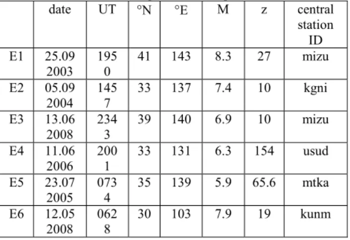
In this study, five earthquakes between 2003–2008 that occurred in Japan with different seismic properties, and the China earthquake in May 2008 are investigated. This earthquakes are composed in Table I as date, time (Universal Time-UT), geographical location (latitude, longitude: in degrees), magnitude in Richter Scale (M), depth (z-km) and central station which is chosen as the nearest recording GPS station to the epicenter [17]. The epicenters which are coded as E1, E2, E3, E4, E5 and E6 represent Hokkaido, Honshu, Honshu, Kyushu, Honshu and Sichuan earthquakes, respectively.
TABLE I :Indicator of date, time, geographical location, magnitude and depth of the earthquakes.
date UT °N °E M z central
station ID E1 25.09 2003 195 0 41 143 8.3 27 mizu E2 05.09 2004 145 7 33 137 7.4 10 kgni E3 13.06 2008 2343 39 140 6.9 10 mizu E4 11.06 2006 2001 33 131 6.3 154 usud E5 23.07 2005 0734 35 139 5.9 65.6 mtka E6 12.05 2008 062 8 30 103 7.9 19 kunm
There have been seven GPS stations that used in this study. These stations are given in Table II. The distance between IGS-GPS stations to the epicenter vary from 35 km to 1000 km.
Tablo II : GPS Stations that are used in the content of the study.
GPS Station Station ID Latitude Longitude
---
Koganei, Japan kgni 35.5 °N 139.4° E
Kashima, Japan ksmv 35.7 °N 140.6° E
Mizusawa, Japan mizu 38.9 °N 141.1° E
Mitaka, Japan mtka 35.4 °N 139.5° E
Tsukuba, Japan tskb 35.9 °N 140.0° E
Usuda, Japan usud 35.9 °N 138.3° E
Yuzh.-Sakh, Russia yssk 46.8 °N 142.7° E
Kunminimumg, China kunm 24.8 °N 102.8° E
The TEC is estimated using the Reg-Est method as IONOLAB-TEC [18,19,20]. There are no significant disturbances in the AE and BE periods [21]. 14 October-02 November 2003 and 23 August-21 September 2005 periods are chosen as DDP. 14 October-03 November 2006 and 27 April-21 May 2006 periods are chosen as QDP [21].
In the first group of the study, in order to compare the behavior of IONOLAB-TEC for the QDP period with those from the DDP, BE and AE periods, an average quiet day TEC estimate (AQDT) for each GPS station is obtained by Equation 2. Equations 4, 5, 6 and 7 are applied AE, BE, QDP and DDP data of seven stations in Table II. It is observed that days of the DDP and AQDT are highly correlated. In the both of the AE and BE periods (EA) and QDP, the correlation coefficients vary between 0.2 and 0.7. The values of EA – AQDT and QD-AQDT are lowly correlated. Difference between minimum and maximum values of KLI, KLD and L2N (D) are larger when the distance of the station decreases and the magnitude of the earthquake increases. If the distance of the station is less far from 150 km, the KLD and the L2N methods select the EA days from the QDP. At the distance less from 150 km, D difference of the KLD, KLI and L2N of DDP-AQDT is greater although there are highly correlation coefficients. For the kunm, KLD, L2N and CCF variations of E6-AQDT, QDP-AQDT and DDP-QDP-AQDT are shown at the Figure 1a, 1b, 1c, respectively. For the mizu, KLD, L2N and CCF variations of E3-AQDT, QDP-AQDT and DDP-AQDT are shown in the Figure 1d, 1e, 1f, respectively. At the E6, which is the greater earthquake than the E3, it is shown that KLD and L2N values of EAP have greater scale than the E3 and KLD and L2N values of both E6 and E3 are greater than the QDP and the DDP.
Figure 1. E6-AQDT, DDP-AQDT and QDP-AQDT of kunm for: a) KLD b) L2N c) CCF and E3-AQDT, DDP-AQDT and QDP-AQDT of mizu for: a)
KLD b) L2N c) CCF.
Figure 2a, and 2b show KLD variations of station mizu for DDP 23 August-21 September 2005, and QDP 14 October-11 November 2006, respectively. It is observed that even on QDP, KLD variation has low ranged scattered distribution. Even on DDP, KLD variation is different from QDP but has smaller level than AE and BE.
8 16 24 0 0.2 0.4 0.6 0.8 1 Days K LD (k unm ) 8 16 24 0 0.01 0.02 0.03 0.04 0.05 Days L2N (k unm ) 8 16 24 -0.9 -0.5 -0.10.1 0.5 0.9 Days C C F (k unm ) 8 16 24 32 0 0.05 0.1 0.15 Days KL D (m iz u) 8 16 24 32 0 0.008 0.016 Days L2 N (m iz u) 8 16 24 32 -0.9 -0.5 -0.10.1 0.5 0.9 Days CC F (m iz u) kunm-epicenter: 678 km mizu-epicenter : 43 km E6 DDP QDP E3 DDP QDP a) b) c) d) e) f)
Figure 2. KLD variations of mizu a) DDP-AQDT b) QDP-AQDT. In the second group of study, the Kullback-Leibler Divergence KLI( Pˆu;d\\ Pˆu;d+1) and KLI( Pˆu;d+1\\ Pˆu;d) , the Kullback-Leibler Distance KLD( Pˆu;d\\ Pˆu;d+1) and
) ˆ \ \ ˆ (
KLDPu;d+1 Pu;d , L2-Norm L2N( Pˆu;d+1\\ Pˆu;d) and Cross Correlation Coefficient ru ;d,d+1 functions are applied to the d and d+1 consequtive days of QDP, DDP, and BE and AE (EAP) periods for each earthquake given at the Table I and each GPS station given at the Table II. For the consequtive days, all of the CCF values of the QDP days vary between 0.8 and 1 and so consequtive QDP days are highly correlated. Consequtive EAP days become low correlated at the nearest stations to the epicenter. At the consequtive days, the values smaller than the 0.8 are %4 at E1, %17 at E2, %3 at E3, %1 at E5, %1 at E6, %5 at QDP and %6 at DDP. The effects of the EAP are observed better than DDP with CCF method for consequtive days. Difference between minimum and maximum values of KLI, KLD and L2N (D) are greater when the distance of the station decreases and the magnitude of the earthquake increases. D values of DDP are similar to the QDP, so KLI, KLD and L2N methods are less sensitive for the consequtive DDP days. Figure 3 shows the KLD and L2N variations of mizu and tskb for the E3. It is shown from Figure 3a and 3b that KLD values for mizu, which has 43 km distance to the epicenter and tskb which has 358 km distance to the epicenter, are very similar. It is also shown from Figure 3c and 3d, L2N values of both stations vary very similar level.
Figure 3. KLD variations of a) mizu b) tskb and L2N variations of c) mizu d) tskb .for consequtive days of E3.
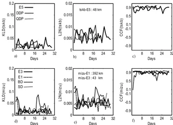
For the tskb, KLD, L2N and CCF variations of E6, QDP and DDP are shown at the Figure 3a, 3b, 3c, respectively. For the mizu, KLD, L2N and CCF variations of E6, QDP and DDP
are shown at the Figure 3d, 3e, respectively. It is shown for mizu that there is no significant difference for the KLD and L2N values of E5, DDP and QDP periods. For the mizu, KLD and L2N values of both E1 and E3 and QDP periods vary very similar level. Both E1 and E3 are the large scaled earthquakes and distances of mizu to the E1and E3 are 392 km and 43 km, respectively. There are no important difference on the KLD and L2N values of E1, E3 and QDP periods. For storm days in the DDP, KLD and L2N values are larger for mizu.
Figure 3. Variations of a) KLD b) L2N c) CCF for consequtive days of E5, DDP and QDP of tskb and variations of a) KLD b) L2N c) CCF.for
consequtive days of E1 E3, DDP and QDP of mizu.
Finally, in group four, the normalized MAQDT is compared with the normalized TEC estimates for QDP, DDP and EAP by using the bounds derived from SQDT in Equation 7 for each earthquake given at the Table I and each GPS station given at the Table II. It is observed that for the MAQDT comparisons and the EAP TEC estimates that are not bounded by STDQDT, especially for those stations that are closer to the epicenter. For the EAP, QDP and DDP of a station, TEC estimates can not be categorized by statistical differentiation because of abundance unbounded values in both of the EAP, DDP and QDP.
IV. CONCLUSION
In this study, the relation between earthquakes and the TEC obtained from GPS is examined. Five earthquakes between 2003-2008 occurred in Japan with different properties and China earthquake in May 2008 are chosen for the purpose. For the statistical analysis, the cross correlation function (CC) which is used in the literature before, and the Kullback-Leibler Divergence (KLD) with L2-Norm (L2N) methods which are used for the first time in this context, are applied to the data sets. It is observed that the CCF, KLD and L2N between the neighbouring GPS stations cannot be used as a definitive earthquake precursor due to the complicated nature of earthquakes and various uncontrolled parameters that effect the behaviour of TEC such as distance to the earthquake epicenter, distance between the stations, depth of the earthquake, strength of the earthquake and tectonic structure of the earthquake. The investigation of CCF, KLD and L2N for the consequtive days for each station indicates that when 0 2 4 6 8 10 12 14 16 18 20 22 24 26 28 30 0 0.01 0.02 0.03 0.04 0.05 0.06 0.07 0.08 0.09 0.1 0.11 0.12 23 August-21 September 2005 KL D( m iz u : DDP -AQDT ) a) 0 2 4 6 8 10 12 14 16 18 20 22 24 26 28 0 0.01 0.02 0.03 0.04 0.05 0.06 0.07 0.08 0.09 0.1 14 October-11 November 2006 KL D (m iz u : QD P-AQ D T ) b) 8 16 24 32 0 0.05 0.1 0.15 0.2 Days KL D (t sk b) 8 16 24 32 0 0.005 0.01 0.015 0.02 Days L2 N (ts kb ) 8 16 24 32 -0.9 -0.5 -0.10.1 0.5 0.9 Days CC F (t sk b) 8 16 24 32 0 0.05 0.1 0.15 0.2 Days KL D (m iz u) 8 16 24 32 0 0.005 0.01 0.015 0.02 Days L2 N (m iz u) 8 16 24 32 -0.9 -0.5 -0.10.1 0.5 0.9 Days CCF (m iz u) E5 DDP QDP E3 BD SD E1 tskb-E5 : 48 km mizu-E1 : 392 km mizu-E3 : 43 km a) b) d) e) c) f) 0 2 4 6 8 1012141618202224262830 0 0.01 0.02 0.03 0.04 0.05 0.06 0.07 0.08 29 May-28 June 2008 K LD( m iz u : c on s eq ut iv ed ay s of E 3) mizu-epicenter : 43 km a) 0 2 4 6 8 1012141618202224262830 0 0.01 0.02 0.03 0.04 0.05 0.06 0.07 0.08 29 May-28 June 2008 K LD( ts k b : c on s eq ut iv e da y s o f E 3) tskb-epicenter : 358 km b) 0 2 4 6 8 1012141618202224262830 0 0.01 0.02 0.03 0.04 29 May-28 June 2008 L2 N( m iz u : c ons equt iv e d ay s of E 3 ) c) 0 2 4 6 8 1012141618202224262830 0 0.01 0.02 0.03 0.04 29 May-28 June 2008 L 2N (t s k b : c on s equ ti v e day s of E 3) d)
similar disturbances occur for days in a row, these methods are inadequate in identifying the disturbance due to earthquakes. The most promising results are obtained for the analysis of Kullback-Leibler divergence between the AQDT and the TEC estimates for the BE. For this group of study, it is observed that the seismic activity before the strong earthquakes have a diurnal disturbance structure which can be distinguished from the ionospheric disturbances due to geomagnetic storms or solar flares. The increasing levels of KLD for preseismic activity is also a promising candidate for further investigation in this direction, especially for those GPS stations that are closer to the epicenter. Similar results are also observed for the MAQDT comparisons and the BE TEC estimates that are not bounded by STDQDT, especially for those stations that are closer to the epicenter. KLD, KLI and L2N are used for the first time in literature for the investigation of earthquake precursor for the first time in literature and the extensive study results indicate that for more reliable estimates further space-time TEC analysis is necessary over a denser GPS network in the earthquake zones.
ACKNOWLEDGMENT
This study is sported by TUBİTAK EEEAG Grant No: 105E171.
REFERENCES
[1] Nayir, H., Ionospheric total Electron Content Estimation
Using GPS Signals (in Turkish), M. Sc. Thesis, Hacettepe
Üniversity, Ankara, Turkey, 2007.
[2] Ondoh, T., “Seismo-Ionospheric Phenomena”, Advances in
Space Research, 26(8): 1267-1272, 2000..
[3] Pulinets, S.A., “Ionospheric precursors of earthquakes; recent
advances in theory and practical applications”, TAO,
15(3):413-435, 2004.
[4] Pulinets, S.A., Gaivoronska, T.B., Contreras L.A. and Ciraolo,
I., “Correlation analysis technique revealing ionospheric precusors of earthquake”, Natural Hazards and Earth Systems
Sciences, 4:697-702, 2004.
[5] Liu J.Y., Chen, Y.I., Pulinets S.A., Tsai Y.B. and Chuo Y.J.,
“Seismo-ionospheric signatures prior to M≥6.0 Taiwan earthquakes”, Geophysical Research. Letters, 27(19):
3113-3116, 2000.
[6] Liu, J.Y., Chuo Y.J., Shan, S.J., Tsai, Y.B., Chen, Y.I., Pulinets,
S.A. and Yu, S.B., “Pre-earthquake ionospheric anomalies registered by continuous GPS TEC measurements”, Annales
Geophysicae, 22(5): 1585-1593, 2004.
[7] Liu, J.Y., Chuo Y.J., Shan, S.J., Tsai, Y.B., Chen, Y.I., Pulinets,
S.A. and Yu, S.B., “Pre-earthquake ionospheric anomalies registered by continuous GPS TEC measurements”, Annales
Geophysicae, 22(5): 1585-1593, 2004.
[8] Chuo. Y.J., Chen, Y.I., Liu, J.Y. and Pulinets, S.A.,
“Ionospheric f0F2 variations prior to strong earthquakes in
Taiwan area”, Advances in Space Research, 27(6):1305-1310,
2001.
[9] Plotkin, V.V., “GPS detection of ionospheric perturbations
before the 13 February 2001 El Salvador earthquake”, Natural
Hazards and Earth Systems Sciences, 3: 249-253, 2003.
[10] Trigunait, A., Parrot, M., Pulinets, S.A.and Li, F., “Variations of the ionospheric electron density during the Bhuj seismic event”,
Annales Geophysicae, 22(12): 4123-4131, 2004.
[11] Fante, R.L., Signal Analysis and Estimation, John Wiley & Sons Inc., New York, 1988.
[12] Papoulis, A., Signal Analysis, McGraw-Hill Book Company, New York, 1977.
[13] Kreyszig, E., Advanced Engineering Mathematics, John Wiley & Sons Inc., New York, 1988.
[14] Inglada, J., “Change detection on SAR images by using a parametric estimation of the Kullback-Leibler Divergence,
IGARSS, 6(21-25): 4104-4106, 2003.
[15] Cho, C., Kim, S., Lee, J. And Lee, DW, “A tandem clustering process for multimodal datasets, European Journal of
Operational Research, 168(3): 998-1008, 2006.
[16] Erol, C.B., Arıkan, F., “Statistical characterization of the ionosphere using GPS signals”, Journal of Electromagnetic
Waves and Applications, 29(13): 373-387, 2005.
[17] http://earthquake.usgs.gov/regional/world
[18] Arıkan, F., Erol, C.B., Arikan O., “Regularized estimation of vertical total electron content from Global Positioning System data”, Journal of Geophysical Research-Space Physics,
108(A12): 1469-1480, 2003.
[19] Nayir, H., Arıkan, F., Arıkan, O. and Erol, C.B., “Total Electron Content Estimation with Reg-Est”, Journal of Geophysical
Research-Space Physics, 112: A11313, 2007.
[20] www.ionolab.org