IMAGE PROCESSING METHODS FOR FOOD
INSPECTION
a thesis
submitted to the department of electrical and
electronics engineering
and the graduate school of engineering and science
of b
˙Ilkent university
in partial fulfillment of the requirements
for the degree of
master of science
By
Onur Yorulmaz
I certify that I have read this thesis and that in my opinion it is fully adequate, in scope and in quality, as a thesis for the degree of Master of Science.
Prof. Dr. Enis C¸ etin (Supervisor)
I certify that I have read this thesis and that in my opinion it is fully adequate, in scope and in quality, as a thesis for the degree of Master of Science.
Assoc. Prof. Dr. U˘gur G¨ud¨ukbay
I certify that I have read this thesis and that in my opinion it is fully adequate, in scope and in quality, as a thesis for the degree of Master of Science.
Asst. Prof. Dr. Sinan Gezici
Approved for the Graduate School of Engineering and Sciences:
Prof. Dr. Levent Onural
ABSTRACT
IMAGE PROCESSING METHODS FOR FOOD
INSPECTION
Onur Yorulmaz
M.S. in Electrical and Electronics Engineering
Supervisor: Prof. Dr. Enis C
¸ etin
January 2012
With the advances in computer technology, signal processing techniques are widely applied to many food safety applications. In this thesis, new methods are developed to solve two food safety problems using image processing techniques. First problem is the detection of fungal infection on popcorn kernel images. This is a damage called blue-eye caused by a fungus. A cepstrum based feature ex-traction method is applied to the kernel images for classification purposes. The results of this technique are compared with the results of a covariance based feature extraction method, and previous solutions to the problem. The tests are made on two different databases; reflectance and transmittance mode image databases, in which the method of the image acquisition differs. Support Vec-tor Machine (SVM) is used for image feature classification. It is experimentally observed that an overall success rate of 96% is possible with the covariance ma-trix based feature extraction method over transmittance database and 94% is achieved for the reflectance database.
The second food inspection problem is the detection of acrylamide on cookies that is generated by cooking at high temperatures. Acrylamide is a neurotoxin
and there have been various studies on detection of acrylamide during the bak-ing process. Some of these detection routines include the correlation between the acrylamide level and the color values of the image of the cookies, resulting easier detection of acrylamide without the need of complex, expensive and time consuming chemical tests. Studies on the subject are tested on still images of the cookies, which are obtained after the cookies are removed from the oven. An active contour method is developed, that makes it possible to detect the cookies inside the oven or possibly on a moving tray, from the video captured from a regular camera. For this purpose, active contour method is modified so that elliptical shapes are detected in a more efficient manner.
Keywords: Fungal Infections on Popcorn Kernels, Cepstrum Features,
¨
OZET
GIDA ˙INCELEMES˙I ˙IC
¸ ˙IN ˙IMGE ˙IS
¸LEME Y ¨
ONTEMLER˙I
Onur Yorulmaz
Elektrik ve Elektronik M¨
uhendisli˘
gi B¨
ol¨
um¨
u Y¨
uksek Lisans
Tez Y¨
oneticisi: Prof. Dr. Enis C
¸ etin
Ocak 2012
Bilgisayar teknolojilerindeki geli¸smelerle birlikte, sinyal i¸sleme teknikleri gıda g¨uvenli˘gi alanında yaygın bir bi¸cimde kullanılmaya ba¸slanmı¸stır. Bu tezde, iki gıda g¨uvenli˘gi problemine imge i¸sleme teknikleri kullanılarak ¸c¨oz¨um ¨uretme amacıyla, yeni y¨ontemler geli¸stirilmi¸stir. Bu problemlerin ilki, patlamı¸s mısır imgeleri ¨uzerinden bir mantar enfeksiyonunun tespit edilmesidir. Mavi-g¨oz (blue-eye) adı verilen bu enfeksiyona bir t¨ur k¨uf sebep olmaktadır. Bu en-feksiyonun sınıflandırılması amacıyla, kepstrum temeline dayanan bir ¨oznitelik ¸cıkarımı y¨ontemi mısır tanelerinin imgelerine uygulanmı¸stır. Bu y¨ontem ile alınan sonu¸clar daha sonra, kovaryans temeline dayanan bir ba¸ska ¨oznitelik ¸cıkarımı y¨onteminin sonu¸clarıyla ve daha ¨onceki ¸calı¸smalarla kıyaslanmı¸stır. Testler iki veritabanı ¨uzerinde ger¸cekle¸stirilmi¸stir; yansıtma ve ge¸cirgenlik t¨ur¨u imge veritabanları, bu iki veri tabanı imgelerin elde edilme tekni˘giyle birbirinden ayrı¸sır. ˙Imgelerin ¨oznitelik sınıflandırması amacıyla, Destek Vekt¨or Makinası (SVM) kullanılmı¸stır. Yapılan deneyler g¨ostermektedir ki, kovaryans matrisi temelli ¨oznitelik ¸cıkarımı y¨ontemiyle, ge¸cirgenlik veritabanında %96, yansıtma veri tabanında ise %94 oranında genel tanıma ba¸sarısı elde edilebilmektedir.
˙Ikinci gıda incelemesi problemi ise y¨uksek sıcaklıklardaki pi¸sirime ba˘glı olarak, bisk¨uvilerde ortaya ¸cıkan akrilamidin tespit edilmesidir. Akrilamid bir n¨orotoksin
olup, pi¸sirim s¨urecinde akrilamidin tespiti i¸cin pek ¸cok ¸calı¸sma mevcuttur. Bu tespit y¨ontemlerinden bir kısmı akrilamid seviyesiyle, bisk¨uvi imgelerindeki renkler arasında kurulabilen ba˘glantıdan yola ¸cıkmakta ve bu sayede akril-amidin karı¸sık, pahalı ve zaman t¨uketen kimyasal testler olmadan kolayca tespit edilmesini sa˘glamaktadır. Ancak bu konudaki ¸calı¸smalar, fırından ¸cıkarılmı¸s bisk¨uvilerin ¨uzerinde test edilmi¸stir. Bisk¨uvileri fırın i¸cerisinde ve hatta hareketli fırın tepsisinden alınan video g¨or¨unt¨us¨u i¸cinde tespit etmek amacıyla, aktif kon-tur temeline dayanan bir y¨ontem geli¸stirilmi¸stir. Bu ama¸cla, elips ¸seklindeki b¨olgelerin daha etkili bir ¸sekilde tespit edebilmek i¸cin, aktif kontur algoritması de˘gi¸stirilmi¸stir.
Anahtar Kelimeler: Mısır Tanelerindeki Mantar Enfeksiyonu, Kepstrum ¨
Oznitelikler, Kovaryans ¨Oznitelikler, Akrilamid, Aktif Kontur Algoritması, Destek Vekt¨or Makinası
ACKNOWLEDGMENTS
I would like to express my gratitude to Prof. Dr. Enis C¸ etin for his supervision, guidance and suggestions throughout the development of this thesis.
I would also like to thank Assoc. Prof. Dr. U˘gur G¨ud¨ukbay and Asst. Prof. Dr. Sinan Gezici for reading, commenting and making suggestions on this thesis.
I would also like to thank to my friends and colleagues, especially Serdar C¸ akır, Osman G¨unay and Kıvan¸c K¨ose for their help through the development of this thesis.
It is a pleasure to express my special thanks to my mother, father and sister for their sincere love, support and encouragement.
Contents
1 Introduction 1
2 Fungus Detection in Popcorn Kernel Images 5
2.1 Related Work on Fungus Detection in Popcorn Kernels . . . 7
2.1.1 2D Cepstrum Analysis . . . 7
2.1.2 Covariance Features . . . 9
2.2 2D Cepstrum Based Methods . . . 10
2.3 Covariance Based Methods . . . 14
2.4 Image Acquisition and Pre-processing . . . 17
2.4.1 Kernel Image Extraction . . . 18
2.4.2 Image Orientation Correction . . . 20
2.5 Classification Method . . . 23
2.6 Experimental Results . . . 23
3 Active Contour Based Method for Cookie Detection on Baking
Lines 30
3.1 The Snake Algorithm . . . 32
3.2 Active Contours Based Elliptic Region Detection Algorithm for Cookie Detection . . . 35
3.2.1 Moving the Snaxels . . . 36
3.2.2 Energy Calculation on Elliptical Contours . . . 40
3.3 The Detection Procedure . . . 42
3.4 Experimental Results . . . 44
3.5 Summary . . . 48
4 Conclusions 49
List of Figures
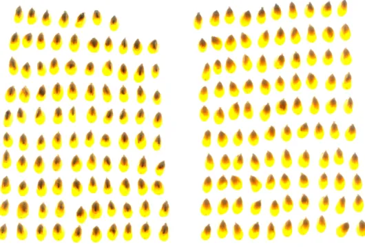
2.1 Images of blue-eye-damaged (left) and undamaged (right) popcorn kernels. . . 6
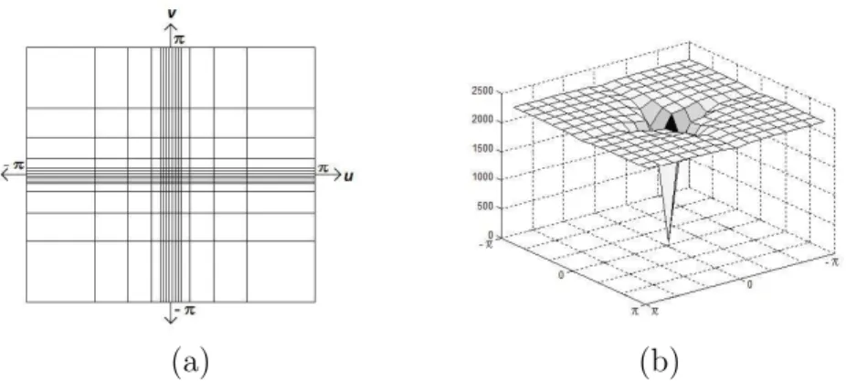
2.2 (a) A sample grid and (b) its corresponding sample weight. . . 11
2.3 The process of applying a grid to the 2D Fourier transform coef-ficients of a given image. . . 11
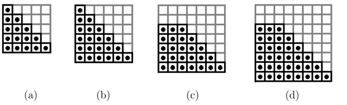
2.4 Illustration of the entry selection from covariance matrices. En-tries extracted from covariance matrices are shown as black dots: Eqs. (2.7), (2.8); Eqs. (2.9), (2.10); Eqs. (2.11), (2.12) and Eqs. (2.13), (2.14) produce the matrices shown in (a), (b), (c) and (d) respectively. . . 16
2.5 (a) Damaged (left) and undamaged (right) popcorn kernel images acquired in the reflectance mode. (b) Damaged (left) and undam-aged (right) kernel images that were obtained in the transmittance mode. . . 18
2.6 Output image of the document scanner for transmittance mode. . 19
2.7 Output image of the document scanner for reflectance mode. . . . 19
2.8 The cropping operation was performed in proportion to the size of each kernel image. . . 20
2.9 (a) The thresholded image of a popcorn kernel and (b) the bound-ary of the kernel obtained from the filtered image. The center of the mass is marked with a (+) sign in both images . . . 21
2.10 (a) The distance from the center of the mass of popcorn to its boundary with respect to angle (Radians) and (b) the derivative of the function in (a) . . . 22
3.1 Cookie inside the oven after 5 minutes of baking. . . 35
3.2 (a)Ellipses with different orientations and (b) ellipses with differ-ent rL
rS values. . . 36
3.3 The initial positions of the snaxels on the contour for N = 32. . . 37
3.4 Any translation of a snaxel should affect other snaxels to keep the elliptical shape. . . 38
3.5 (a) The contour sits on a part of the boundary and (b) extending toward the center of the bright region causes some snaxels to leave the boundary and increases total energy. . . 39
3.6 (a) Visualization of dj displacement vectors for each jth snaxel.
(b) The gj vectors for the same snaxels (N = 16). . . . 40
3.7 (a) The contour sits on a part of the boundary. (b) Extending toward the center of the bright region causes some snaxels to leave the boundary. (c) The translation of all snaxels in the direction of
gj moves the snaxels back to the boundaries decreasing the total
energy. . . 40
3.8 An image of two cookies being baked inside the oven . . . 43
3.10 Detection results on the image taken from 1st video at the 5th minute. . . 46
3.11 Detection of the cookie region with (a) the proposed method and (b) with the ordinary active contour method [1]. . . 46
List of Tables
2.1 The sizes of grids and the number of resulting features without the addition of intensity based feature. . . 24
2.2 Healthy, damaged and overall recognition rates of Mellin– cepstrum based classification method on transmittance and re-flectance mode popcorn kernel images. . . 24
2.3 Healthy, damaged and overall recognition rates of mel–cepstrum based classification method on transmittance and reflectance mode popcorn kernel images. . . 25
2.4 Comparison of the kernel recognition success rates using the prop-erty vectors defined in Eqs. 2.7 – 2.14 to derive image features from transmittance-mode images. . . 26
2.5 Comparison of the kernel recognition success rates using the prop-erty vectors defined in Eqs. 2.7 – 2.14 to derive image features from reflectance-mode images . . . 26
3.1 Active contour algorithm . . . 34
3.2 Active contour based algorithm for elliptical region detection . . . 42
Chapter 1
Introduction
Every year, millions of people experience serious and sometimes fatal health problems following consumption of unsafe or contaminated food. The contami-nation may involve foodborne disease or chemical hazards. Furthermore, billions of dollars are lost annually in the food industry to insect damage and inefficient production and inspection processes. The goal of this thesis is to introduce image processing techniques and provide solutions to some of the challenges that arise in food inspection. The traditional food-inspection techniques which rely on sample collection and subsequent offline analysis in a laboratory are slow in inspection and thus inefficient. However, with the advances in computers, newer approaches that use nondestructive methods to measure various quality parameters of food products in real time can be implemented.
In this thesis, two different cases of food inspection problems are investigated. The first problem is the detection of fungal damaged popcorn kernels that are hard to separate considering the sizes and the amounts of the kernels. All grain kernels are vulnerable to fungal infection, if not dried quickly before loading into a storage bin. Popcorn poses a particularly difficult problem in that the drying rate must not be too fast and the level of kernel moisture not reduced too much
or the kernels will not pop. Thus, popcorn processors have the difficult task of balancing the drying rate of incoming popcorn with the risk of inadequate drying and possible fungal infection. One type of prevalent fungus that infests popcorn at harvest time is the Penicillium fungi which causes a dark blue blemish on the germ of popcorn commonly referred to as “blue-eye” damage [2]. While this type of infection is not a health risk, it does produce very strong off flavors, causing consumers to reject the popcorn. Given the difficulty of balancing drying rate while maximizing the number of kernels that will pop, a certain percentage of blue-eye damaged popcorn kernels are inevitable every year. The blemish caused by the fungal infection is small and currently no automated sorting machinery can detect it. Thus, new methods for detecting and removing this type of defect is needed by the popcorn industry. It is possible to detect popcorn kernels infested by the fungi using image processing.
In this thesis, for the purpose of detection of fungus in popcorn kernels, two different methods are developed and compared to each other. The first method is based on two dimensional (2D) cepstrum. Cepstrum based methods are used in order to match images which are scaled versions of each other [3]. Addition-ally a non-uniform grid is used to reduce the total number of cepstral features and weights are applied to emphasize the important frequency components. It is observed that the method is effective for the detection of fungus. Fungus de-tection results of the cepstrum method is then compared with the results of the covariance based method which extracts features from groups of pixels of given image. A property vector is built from the intensity values, color values, first and second derivative values of intensity and color values, and the coordinate values. The covariance matrix of these property vectors is also found to be distinctive and is used to detect the existence of the fungus in popcorn kernels.
The second problem that is investigated is the detection of acrylamide level in cookies. Food inspection for acrylamide detection involves the detection of this
well-known neurotoxin in cookies using image processing. Acrylamide is classi-fied as a probable human carcinogen by the International Agency for Research on Cancer (IARC). In 2002, Swedish researchers [4] found that potato chips and French fries contain levels of acrylamide that are hundreds of times higher than those considered safe for drinking water by the Environmental Protection Agency (EPA) and the World Health Organization (WHO). Currently, chemical methods are used to estimate acrylamide levels in baked or fried foods. These methods usually entail extraction of acrylamide from food and purification of the extract prior to analysis by liquid chromatography or gas chromatography coupled with mass spectrometry. The associated analytical systems are very ex-pensive and not common in food inspection laboratories. On the other hand, chemical reactions on the surface of foods are responsible for the formation of color and acrylamide, giving them an opportunity to correlate with each other. A simple color-measurement device measuring CIE Lab parameters cannot be used to estimate meaningful parameters for acrylamide levels in a given food item because the color is not homogeneously distributed over the surface of the food item. Fortunately, the image of a food item can be analyzed in real time, and meaningful features correlated with the acrylamide level can be estimated from the image of the food item. After the cooking process, bright yellow, brown-ish yellow, and dark brown regions are clearly visible in cookie images. It is experimentally observed a high correlation between the normalized acrylamide level and the normalized ratio of brownish yellow regions to the total area in a cookie. This observation indicates that, by installing cameras in production lines, and analyzing cookie images in real time, one can detect and remove cook-ies with brownish yellow regions from a production line, significantly reducing the acrylamide levels that people consume.
The rest of the thesis is organized as follows. In Chapter 2, fungus detection problem in popcorn kernel images is investigated with cepstrum and covariance based methods. The procedure, classifiers, dataset and simulation results are
given in the same chapter. In Chapter 3, a cookie detection algorithm in video frames of a production line is developed. After detecting the cookie, it is possible to check its color to reject it or accept it. This will help reduce the average acrylamide level of a production line. Conclusions are made and contributions are stated in the last chapter.
Chapter 2
Fungus Detection in Popcorn
Kernel Images
The drying of grain kernels is an important issue in agriculture that requires precise timing. Grain kernels that are not dried properly may become infected by fungi, thereby greatly reducing the economic value of the product. In popcorn kernels, one of these problematic infections is called blue-eye damage and is caused by fungi from the Penicillium genus. Fungi can spread over the kernels after harvesting if they are not dried rapidly enough. However, popcorn cannot be dried rapidly with the use of high heat because it may crack and be unable to pop. If a balance between the time until storage and the time for proper drying is not achieved successfully, kernels may still be wet when they are sent for binning, thereby creating a favorable environment for fungal infections to spread. Blue-eye damage changes the taste of popped kernels and causes consumers to reject them, reducing the consumption of popcorn and resulting in economic losses for the popcorn industry. Although damaged kernels do not occur with high frequency, only a few infected kernels are required for consumers to stop buying popcorn.
Figure 2.1: Images of blue-eye-damaged (left) and undamaged (right) popcorn kernels.
Blue-eye-infected popcorn kernels have a small blue blemish on the kernels at the center of the germ. This blemish makes it possible to approximate the location of the infection and to detect infected kernels from images taken by regular color cameras. Figure 2.1 shows images of undamaged and damaged popcorn kernels that were obtained with a Canon Powershot G11 digital camera.
There have been various studies on the subject of separating blue-eye-damaged and unblue-eye-damaged kernels. Pearson developed a machine to detect the damaged kernels as they slide down a chute [2]. Three cameras located around the perimeter of the kernel simultaneously obtained images while a Field-Programmable Gate Array (FPGA) processed each image in real time. The array looked for rows in the image matrix in which the intensity values were greater at the borders of the germ and lower in the middle of the germ. The detection of this valley-like shape in image intensity values along a line of the image was used to confirm the existence of blue-eye damage. In this approach, the red channels of the images of the kernels were used, because the kernels are red-yellow, and the damage is more visible in this channel. However, the accuracy of this system, 74 % for the blue-eye damaged popcorn, was not adequate for the system to be useful for the popcorn industry.
The rest of the chapter is organized as follows. In Section 2.1, related work on fungus detection in popcorn images are presented. In Section 2.2, the cepstrum-based method that is developed is presented with details. Covariance-cepstrum-based fea-ture extraction methods that are applied to popcorn damage detection problem are presented in Section 2.3. The image acquisition steps for building the train-ing and test databases are detailed in Section 2.4. SVM classification method that is used in this thesis is reviewed in Section 2.5, and experimental results are presented in Section 2.6.
2.1
Related Work on Fungus Detection in
Pop-corn Kernels
In this part of the thesis, the blue-eye damaged popcorn kernel detection prob-lem is investigated through various image processing techniques. Two different feature extraction methods are developed and applied to the popcorn kernel images. The methods that are experimented are based on the cepstrum and co-variance features. In Section 2.1.1, the cepstrum method is introduced and the improvement made on this thesis is presented briefly which is explained in detail in Section 2.2. In Section 2.1.2, covariance based methods are presented that will be used in Section 2.3.
2.1.1
2D Cepstrum Analysis
Mel-cepstral analysis is a major tool for sound processing including important speech applications such as speech recognition and speaker identification [5], [6]. The two dimensional (2D) extension of the analysis method is also applied to images to detect shadows, remove echoes and establish automatic intensity
control [5], [7], and [8]. Recently the 2D cepstral analysis was applied to image feature extraction for face recognition [9] and man made object classification [10].
The 2D mel-ceptrum is defined as the 2D inverse Fourier transform of the logarithm of the magnitudes of 2D Fourier transform of an image. Cepstral analysis is useful when comparing two similar signals in which one of them is a scaled version of the other one. This is achieved through the logarithm operation.
As it is based on the magnitude of the Fourier transform, mel-cepstrum is shift invariant. If a given image is translated version of another, only the phase of the Fourier coefficients change. Therefore two images can be compared to each other using only the Fourier transform magnitude based mel-cepstrum.
The Mellin-ceptrum is similar to the mel-cepstrum method, where the differ-ence is that a log-polar conversion is applied to the logarithm of the magnitudes of the Fourier coefficients to provide rotational invariance. In log-polar conver-sion, the magnitude values which are represented in Cartesian coordinate indexes are converted to polar coordinate system representation. As a result of this con-version, rotational differences become shift differences. Shift differences can be taken out by Inverse Discrete Fourier Transform (IDFT) that is followed by an absolute value operation so that the Mellin-cepstrum of an image becomes rota-tion invariant.
In [10], a grid technique is introduced to reduce the number of total features in the classification phase. A grid is a set of bins with different sizes covering the matrix of Fourier transform coefficients. By averaging the Fourier coefficients in bins, it is possible to reduce the number of feature parameters representing a given image. In [10] this combination is achieved through power averaging.
As a part of this thesis, popcorn kernel images are represented in mel– and Mellin-cepstral domain. The details of the implementation procedure is given in Section 2.2.
2.1.2
Covariance Features
Covariance features are proposed and used for object detection by Tuzel et al. [11]. In [12] and [13], covariance features are applied to synthetic aperture radar (SAR) images for object detection purposes. Covariance features are introduced as a general solution to object detection problems in [11]. Seven image-intensity-based parameters were extracted from the pixels in image frames, and their covariance matrix was used as a feature matrix to represent an image or an image region. The distance between two covariance matrices was computed using generalized eigenvalues in [11]. However, this operation is computationally costly. To adapt the algorithm to real-time processing, the upper diagonal elements of the covariance matrix are used as features [12], [14].
In [11] the covariance feature extraction methods are applied to object detec-tion in videos. [15] used this method for image texture classificadetec-tion and forest fire smoke detection in videos. Damaged popcorn kernels have an image texture that is different from that of undamaged kernels; therefore, it is proposed that a texture classification method can be used to distinguish damaged kernels from undamaged kernels. The first step is to calculate the property vector of each pixel in the image. Next, the covariance matrix of all property vectors is obtained to represent an image or an image region. Typically, the property vector Θi,j of the
(i, j)’th pixel is composed of gray-scale intensity values or color-based properties and their first and second derivatives. After the property vectors are computed, the covariance matrix of an image is estimated by the following operation:
ˆ Σ = 1 N − 1 ∑ i ∑ j (Θi,j− Θ)(Θi,j− Θ)T (2.1)
where, ˆΣ is the estimated covariance matrix; N is the number of pixels in the region; Θi,j is the property vector of the pixel located at coordinates i and j; and
Θ is the mean of Θi,j in the given image region, which is calculated as follows:
Θ = 1
N
∑∑
The property vectors are defined to include various properties of the pix-els. These properties may be based on intensity and color values, first and second derivatives of intensity or color values and the coordinate information. The property vector elements used in this thesis will be detailed in Section 2.3. The covariance feature extraction from the covariance matrices of these property vectors will also be introduced in the same section.
2.2
2D Cepstrum Based Methods
In this section, popcorn kernel images are represented in 2D mel- and Mellin-cepstral domain. The 2D extension of the Mellin-cepstral analysis is defined as follows:
˜
x(p, q) = F2−1(log(|X(u, v)|2)) (2.3) where p and q are the 2D cepstrum domain coordinates, F2−1 denotes the inverse 2D Fourier transform, and X(u, v) denotes the Fourier transform coefficient of a given signal x at frequency locations given by u and v. In practice the Fast Fourier Transform (FFT) is used to calculate the Fourier transform of a signal while the Inverse Fast Fourier Transform (IFFT) is used to calculate the inverse Fourier transform.
As an extension of 2D cepstral analysis method, the mel-cepstrum method applies grids to the Fourier transform of the signal and sums the energies of Fourier transform components within grid cells before computing the logarithm [9]. The goal of this is to reduce the size of the data and to emphasize some frequency bands. In the mel-cepstrum method, there is also a weighting process that emphasizes the important frequency values and reduces the contribution of the noise to the final decision. Eight different grids are designed and studied for best grid selection. The weights are also selected to increase the higher frequency components’ contribution. The DC value was multiplied by a small weight value where other high frequency grid cell energies are multiplied by
(a) (b)
Figure 2.2: (a) A sample grid and (b) its corresponding sample weight.
Figure 2.3: The process of applying a grid to the 2D Fourier transform coefficients of a given image.
relatively larger numbers. A sample grid and corresponding weight matrix are shown in Figure 2.2.
In each grid cell the Fourier transform magnitudes are summed as follows;
g(m, n) = 1 size(B(m, n))
∑
u,v∈B(m,n)
|X(u, v)| (2.4)
where g(m, n) is the value of the grid in coordinate locations m and n, and
B(m, n) denotes the (m, n)-th grid bin. The size(B(m, n)) gives the total number
of frequency components that are in the bin B(m, n). Thus, the procedure of grid usage on the Fourier transform of an image can be illustrated as in Figure 2.3.
After finding the grid values, the cepstral feature parameters are calculated as follows:
˜
x(p, q) = F2−1(log(|g(m, n)|)) (2.5) Thus, the mel-cepstrum procedure is summarized in six steps:
• 2D Fourier transform of the given NxN image matrices are taken. Here N
is selected to be a power of 2 such that N=2k where k is an integer. The images are padded with zeros before Fourier transform so that the width and height values are increased to N.
• The absolute value of the Fourier coefficients are taken to apply grids. The
grid bins are placed so that each frequency component resides inside a certain bin according to the grid implementation.
• The grid features are taken by averaging. In this part of the procedure,
the average of the elements of each bin are calculated. Then the averages are taken to be single features to be used in the process. While taking the features, their locations in the grid are also untouched, so that an MxM grid features matrix is calculated.
• Each component of the grid features matrix is multiplied by a coefficient
taken from designed weights matrix. 5. Logarithm of the grid features are taken to make use of the cepstral analysis method.
• The inverse 2D Fourier transform is taken to find the final mel-cepstrum
features.
After taking the absolute values of 2D Fourier coefficients, the procedure becomes translation invariant, however, it is still sensitive to rotational transfor-mations. The rotational invariance is achieved in another method called Mellin-cepstrum that is an extension of the mel-Mellin-cepstrum. In Mellin-Mellin-cepstrum, after the application of grid process, a log-polar conversion is applied to achieve rotational invariance. The log polar conversion is defined as;
p(r, θ) = g(ercos(θ), ersin(θ)), (2.6) where g(m, n) is the calculated average power of the Fourier transform inside the bin at coordinates m and n: the grid value, p is the frequency coefficient
representation in polar coordinates and r and θ are the parameters of polar coordinate system. Here the parameters of the grid coefficient matrix may be non-integer values. This problem can be solved by finding the approximation of the values in those points through interpolation. The points in polar space that correspond to the outside of the Fourier matrix can be taken as zero.
The log-polar procedure is also given as follows:
• 2D Fourier transform of the given NxN image matrices are taken. Here N
is selected to be a power of 2 such that N=2k where k is an integer. The images are padded with zeros before Fourier transform so that the width and height values are increased to N.
• Logarithm of the absolute value of the Fourier coefficients are taken to
make use of the cepstral analysis method.
• Grids are applied to resulting features. The grid bins are placed so that
each frequency component resides inside a certain bin according to the grid implementation.
• The grid features are taken by averaging. In this part of the procedure,
the average of the elements of each bin are calculated. Then the averages are taken to be single features to be used in the process. While taking the features, their locations in the grid are also untouched, so that an MxM grid features matrix is calculated.
• Each component of the grid features matrix is multiplied by a coefficient
taken from designed weights matrix.
• Log-polar transformation is applied to make the classification method
ro-tation invariant.
• To remove imaginary parts in coefficients, absolute values of the resulting
coefficients are taken.
2.3
Covariance Based Methods
In this section, popcorn kernel images are represented by covariance and corre-lation matrix based features. For this purpose, various property vectors were tested and the classification performances of different combinations of properties were compared. The gray-scale intensity values may not contribute significantly to the popcorn classification results. However, the property values from separate color channels may improve the recognition rates. As was performed by Tuzel et al. [11], the color and gray-scale intensity-based properties were combined to build property vectors and were shown to give superior classification results in some applications.
In addition to the red- and blue-channel pixel values, the contributions of the first and second derivative values in the vertical and horizontal directions were tested by including them in the property vectors. The pixel locations were included and excluded in vector definitions to test their contributions to the results. The eight property vectors that were tested are given in Eqs. (2.7)-(2.14) as follows: Θi,j = [ R(i, j), ∂R(i, j) ∂x
, ∂R(i, j)∂y , ∂2R(i, j)∂x2
, ∂2R(i, j)∂y2 ]T (2.7) Θi,j = [ R(i, j), ∂B(i, j) ∂x
, ∂B(i, j)∂y , ∂2B(i, j)∂x2
, ∂2B(i, j)∂y2 ]T (2.8) Θi,j = [
R(i, j), B(i, j), ∂R(i, j) ∂x
, ∂R(i, j)∂y , ∂2R(i, j)∂x2
, ∂2R(i, j)∂y2 ]T (2.9) Θi,j = [
R(i, j), B(i, j), ∂B(i, j) ∂x
, ∂B(i, j)∂y , ∂2B(i, j)∂x2
, ∂2B(i, j)∂y2
Θi,j =
[
i, j, R(i, j), ∂R(i, j) ∂x
, ∂R(i, j)∂y , ∂2R(i, j)∂x2
, ∂2R(i, j)∂y2 ]T (2.11) Θi,j = [ i, j, R(i, j), ∂B(i, j) ∂x
, ∂B(i, j)∂y , ∂2B(i, j)∂x2
, ∂2B(i, j)∂y2 ]T (2.12) Θi,j = [
i, j, R(i, j), B(i, j), ∂R(i, j) ∂x
, ∂R(i, j)∂y , ∂2R(i, j)∂x2
, ∂2R(i, j)∂y2 ]T (2.13) and Θi,j = [
i, j, R(i, j), B(i, j), ∂B(i, j) ∂x
, ∂B(i, j)∂y , ∂2B(i, j)∂x2
, ∂2B(i, j)∂y2
]T (2.14) where R(i, j) and B(i, j) are, respectively, the red- and blue-channel color values of the pixel located at coordinates i and j. The first and second derivatives of the red- and blue-channel values are calculated by convolution with the [−1, 0, 1] and [1,−2, 1] filters, respectively; i.e., the image is horizontally (vertically) convolved with the [−1, 0, 1] vector to compute the horizontal (vertical) derivative. The resulting covariance matrices has sizes of 5× 5 for Eqs. (2.7) and (2.8), 6 × 6 for Eqs. (2.9) and (2.10), 7× 7 for Eqs. (2.11) and (2.12), and 8 × 8 for Eqs. (2.13) and (2.14), respectively. Coordinate values are also included in the feature vectors (2.11), (2.12), (2.13) and (2.14) because the blue-eye damage is usually located at the center of the popcorn kernel image. As a result, index-sensitive covariance parameters can be obtained from the feature matrix. Feature vectors (2.7) - (2.10) produced location-invariant feature matrices.
The covariance matrices of the image and video regions in either 2D or 3-dimensional spaces can be used as representative features of an object, and they can be compared for classification purposes. As stated in [11], covariance features do not lie in Euclidean space, and, therefore, the distances between covariance matrices cannot be calculated as if they are in Euclidean space. To overcome this problem, [16] developed a method based on generalized eigenvalues and used it to measure the similarity of matrices in [11]. However, this operation was computationally costly, and because real-time applications require computational
(a) (b) (c) (d)
Figure 2.4: Illustration of the entry selection from covariance matrices. Entries extracted from covariance matrices are shown as black dots: Eqs. (2.7), (2.8); Eqs. (2.9), (2.10); Eqs. (2.11), (2.12) and Eqs. (2.13), (2.14) produce the matrices shown in (a), (b), (c) and (d) respectively.
efficiency, the elements of the covariance matrices were calculated as if they were feature values in Euclidean space [14].
In [14], an SVM [17] was used as the classifier. The presence of the five ele-ments in the property vectors that were defined in Eqs. (2.7) and (2.8) results in 5× 5 = 25 features in the covariance matrix. Similarly, covariance matrices constructed from the property vectors in Eqs. (2.9) and (2.10) has 36 features; Eqs. (2.11) and (2.12) produce 49 features, and Eqs. (2.13) and (2.14) produce a total of 64 features. However, because the covariance matrices are symmetrical with respect to their diagonal elements, only the upper or lower diagonal ele-ments were included in the classification process. The eleele-ments of the covariance matrices corresponding to the covariance values of xy, xx and yy (at locations (1, 1), (1, 2) or (2, 1), and (2, 2), respectively) were omitted from the covariance matrices that were calculated by Eqs. (2.11)–(2.14) because those values do not provide any relevant information about the distributions of intensities. Figure 2.4 illustrates the entry selection process from covariance matrices that is computed using Eqs. (2.7)–(2.14).
In addition to the covariance matrix features, correlation coefficient descrip-tors that were defined in [18] were also applied to the classification problem. Correlation coefficient-based features were obtained by normalizing the covari-ance parameters from Eqs. (2.7)–(2.14) that were calculated from image pixel
values. The correlation coefficient C(a, b) of the (a, b)-th entry of the correlation coefficient matrix was calculated as follows:
C(a, b) = √ Σ(a, b) , a = b √ Σ(a,b) √ Σ(a,a)√Σ(b,b) , otherwise , (2.15)
where Σ(a, b) is the (a, b)th entry of the covariance matrix ˆΣ:
Σ(a, b) = 1 N − 1 ∑ i ∑ j
Θi,j(a)Θi,j(b)− cN(a, b), (2.16)
where Θi,j(a) is the property value located in the ath index of the property vector
of the pixel with the coordinate values i and j, and
cN(a, b) = 1 N ( ∑ i ∑ j Θi,j(a) ) ( ∑ i ∑ j Θi,j(b) ) . (2.17)
2.4
Image Acquisition and Pre-processing
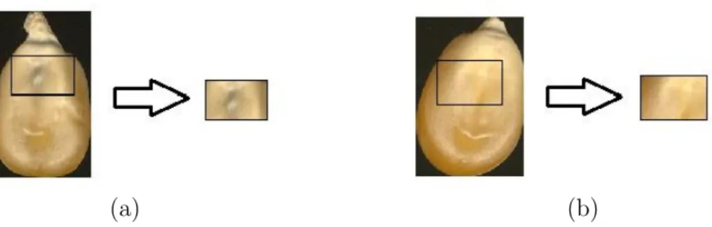
The datasets that are used with cepstrum- and covariance-based features are ob-tained using a document scanner (Expression 1680, Epson America, Long Beach, CA). There are two different types of popcorn images in these datasets: the first set includes reflectance mode images, and the second set includes transmittance mode images. Reflectance images are similar to regular camera images. In this mode, the light reflected from the kernels is captured. In the transmittance mode, the light that passes through the popcorn kernels is captured. In many kernels, blue-eye damage is more visible in transmittance-mode images than in reflectance-mode images. Examples of transmittance-mode and reflectance-mode images are shown in Figure 2.5.
(a) (b)
Figure 2.5: (a) Damaged (left) and undamaged (right) popcorn kernel images acquired in the reflectance mode. (b) Damaged (left) and undamaged (right) kernel images that were obtained in the transmittance mode.
2.4.1
Kernel Image Extraction
The dataset that is used in this thesis includes various popcorn kernels from previous harvest years. This provides further robustness to the algorithms toward the changes relative to the year of harvest and the seed variety. This dataset contains 398 healthy and 510 damaged kernels. The kernels are grouped and kernel images are acquired through a document scanner with a resolution of 4780× 2950. Example images of transmittance and reflectance modes are shown in Figures 2.6 and 2.7, respectively. After this step, in order to extract the images of single kernels, a Matlab program processed on the red channel of the image. Using this program, a threshold is applied to red channel and connected pixels that exceeds this threshold are selected as single kernels for reflectance mode. For transmittance mode, pixels that are less than this threshold are selected to be the kernel pixels. For transmittance and reflectance images, these threshold values are selected accordingly. As a result images of single kernels are achieved and the examples are shown in Figure 2.5.
As can be seen in Figure 2.5, the background is included in a typical popcorn kernel image because the image data was obtained in a rectangular manner. To reduce the effects of the background pixel intensities, the approximate location of possible blue-eye damage was cropped from each popcorn image. This operation
Figure 2.6: Output image of the document scanner for transmittance mode.
Figure 2.7: Output image of the document scanner for reflectance mode. 8
(a) (b)
Figure 2.8: The cropping operation was performed in proportion to the size of each kernel image.
was performed in proportion to the size of the kernel image. Because blue-eye damage is mostly located in the upper part of a popcorn kernel, the left and right margins were set to be 20% of the original image width, whereas the top margin was set to 25% of the image height, and the bottom margin was set at 50% of the image height, as shown in Figure 2.8. Using this approach, a small rectangular region of each image was extracted.
As a result of this kernel image extraction and the cropping process, images of different sizes and shapes were obtained. Typically, the cropped sizes of ker-nel images were 100 by 70 pixels. At this point, kerker-nel images are customized according to the kernel image detection algorithm. Such as, the images are ex-tended to 256 by 256 pixels for cepstral feature extraction methods, in order to make use of the FFT algorithm. Since extending the images by adding zeros would cause high frequency values on the borders, the last rows and the last columns are copied and so the images are stretched from the borders. Because the covariance and correlation features do not depend on the number of pixels, images need not be the same size and thus they are not extended for covariance feature extraction.
2.4.2
Image Orientation Correction
Kernels are oriented manually on the document scanner such that the tips of the germ were on the upper side of the image for the construction of the dataset of
(a) (b)
Figure 2.9: (a) The thresholded image of a popcorn kernel and (b) the boundary of the kernel obtained from the filtered image. The center of the mass is marked with a (+) sign in both images
this thesis. However, in real-time sorting applications, popcorn kernels may have different orientations. Therefore, the direction detection algorithm presented by [19] was implemented to detect the tip of the kernel. This algorithm is based on estimating the contour of the kernel and determining the tip of the popcorn using the derivative of the contour.
The steps of this algorithm consisted of thresholding the kernel images from the background and determining the boundaries of the popcorn kernels; the center of the mass for the popcorn bodies was estimated using the thresholded kernel images, as shown in Figure 2.9.
In order to detect the edges of the kernel, the thresholded image was high pass filtered using the filter with 2D weights that are given as follows:
hHP[m, n] = −0.0625 −0.125 −0.0625 −0.125 0.75 −0.125 −0.0625 −0.125 −0.0625 (2.18)
Filtering produces the image shown in Figure 2.9 (b). In Figure 2.9 (b), the absolute value of the filter output is shown. At this stage, the boundary pixels of
(a) (b)
Figure 2.10: (a) The distance from the center of the mass of popcorn to its boundary with respect to angle (Radians) and (b) the derivative of the function in (a)
the kernel were clearly visible, and detecting these pixels was straightforward. A 1-dimensional distance function representing the distance between the boundary pixels from the center of the mass of the kernel was calculated, as shown in Figure 2.10 (a). In this distance function, the 360o angular range around the
kernel was covered in 64 steps. In almost all kernel images, the tip of the kernel corresponded to the maximum of this function. The tip of the popcorn kernel should also correspond to the highest curvature. The function in Figure 2.10 (a) was processed using the high pass filter with the impulse response of Eq. 2.19 to determine the angle with the highest curvature.
As shown in Figure 2.10 (b), the maximum value had the highest derivative. Because the direction of the tip is known, the image of the popcorn was rotated so that the tip pointed to the top of the image before extracting the germ portion of the image.
2.5
Classification Method
For both the covariance and correlation methods, the classification of kernels as blue-eye damaged or non-damaged was achieved through an SVM, and the results were compared with those obtained using the mel-cepstrum-based method. The SVM is a supervised classification technique that was developed by Vladimir Vapnik [17]. The algorithm was implemented as a Matlab library in [20] and was also used for this study. The SVM algorithm projects the points in a space into higher-dimensional spaces in which a superior differentiation between classes can be achieved using the Radial Basis Function (RBF) Gaussian kernel. Next, the algorithm finds vectors from the higher-dimensional space that are on the borders of class clouds called support vectors and, using these vectors, classifies the remaining samples. For this work, the RBF kernel of the SVM algorithm was applied.
As it is a supervised classification method, an SVM must be trained using previously labeled data. For this work, the datasets for training and testing the SVM were randomly divided into subsets of equal size, and the SVM was trained and tested accordingly.
2.6
Experimental Results
Cepstrum and covariance based features are experimented on the databases that are introduced in Section 2.4. While testing the images with the cepstral features, three intensity based features are added to the feature vector that is acquired from the cepstral features. These additional features includes, the mean of the pixel intensity values in red channel, the difference between mean and the minimum of the intensity values and the number of pixels with intensity values less than a given threshold i. The value i is determined by a Matlab program that finds
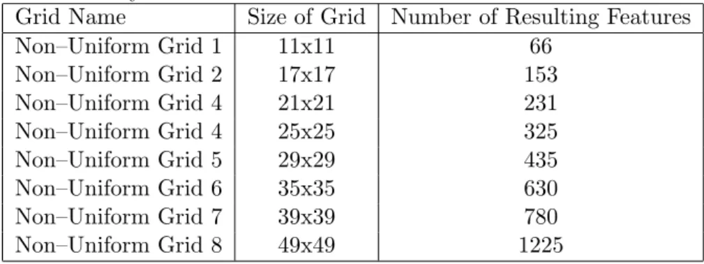
the best i to maximize the detection rate. The second parameter related to the minimum intensity value is ignored in the tests with reflectance images since it reduced success rates because of the dark background. The overall success was also calculated by weighting the results according to the number of test images of two different kernel classes. The non-uniform grid properties are given in Table 2.1.
Table 2.1: The sizes of grids and the number of resulting features without the addition of intensity based feature.
Grid Name Size of Grid Number of Resulting Features
Non–Uniform Grid 1 11x11 66 Non–Uniform Grid 2 17x17 153 Non–Uniform Grid 4 21x21 231 Non–Uniform Grid 4 25x25 325 Non–Uniform Grid 5 29x29 435 Non–Uniform Grid 6 35x35 630 Non–Uniform Grid 7 39x39 780 Non–Uniform Grid 8 49x49 1225
From the results of the tests, two different tables are obtained for cepstral fea-tures. Table 2.2 illustrates the success rates of Mellin–cepstral features for both transmittance and reflectance mode popcorn kernel images. Table 2.3 illustrates the success of mel–cepstral features.
Table 2.2: Healthy, damaged and overall recognition rates of Mellin–cepstrum based classification method on transmittance and reflectance mode popcorn ker-nel images.
Reflectance Success Rate (%) Transmittance Success Rate (%) Grid Name Overall Healthy Damaged Overall Healthy Damaged Non–Uniform Grid 1 73.8571 82.2785 62.9508 95.3571 96.4557 93.9344 Non–Uniform Grid 2 81.2143 82.4051 79.6721 93.4286 94.9367 91.4754 Non–Uniform Grid 3 78.7857 84.0506 71.9672 93.2143 94.6835 91.3115 Non–Uniform Grid 4 80.2857 83.0380 76.7213 93.6429 93.9241 93.2787 Non–Uniform Grid 5 76.7857 79.7468 72.9508 91.5000 93.6709 88.6885 Non–Uniform Grid 6 78.2143 81.0127 74.5902 91.2143 91.3924 90.9836 Non–Uniform Grid 7 77.7143 79.7468 75.0820 92.0714 91.8987 92.2951 Non–Uniform Grid 8 73.1429 77.2152 67.8689 92.2857 95.1899 88.5246
Table 2.3: Healthy, damaged and overall recognition rates of mel–cepstrum based classification method on transmittance and reflectance mode popcorn kernel im-ages.
Reflectance Success Rate (%) Transmittance Success Rate (%) Grid Name Overall Healthy Damaged Overall Healthy Damaged Non–Uniform Grid 1 78.2857 83.0380 72.1311 92.2143 96.0759 87.2131 Non–Uniform Grid 2 81.5000 83.1646 79.3443 93.0714 95.9494 89.3443 Non–Uniform Grid 3 82.0714 83.4177 80.3279 94.0714 97.2152 90.0000 Non–Uniform Grid 4 83.3571 86.8354 78.8525 92.1429 96.5823 86.3934 Non–Uniform Grid 5 82.3571 84.8101 79.1803 93.2143 97.0886 88.1967 Non–Uniform Grid 6 81.5000 86.4557 75.0820 92.9286 97.4684 87.0492 Non–Uniform Grid 7 80.2143 82.6582 77.0492 92.2857 97.3418 85.7377 Non–Uniform Grid 8 81.3571 84.0506 77.8689 92.6429 96.9620 87.0492
The experiments showed that the transmittance images are more suitable for the classification of blue-eye damaged popcorn kernel images from the undam-aged ones. In general, Mellin-cepstrum resulted the greatest recognition rate when Non-Uniform Grid 1 is applied to cepstral features. However in general, when compared to mel-cepstrum, Mellin-cepstrum did not have a significant advantage since the kernels in the images were oriented and thus orientation-invariance was not necessary. On the other hand, mel-cepstrum had a greater recognition rate for reflectance mode images. This is important because the transmittance mode images are harder to obtain compared to reflectance mode. Thus the success rate increase in reflectance mode is considered to be more im-portant.
The same dataset is also experimented with the covariance and correlation features. These features are extracted using the eight different property vector types that were defined in Eqn. 2.7 – 2.14. As it was in the case of cepstrum-based features, the overall success for covariance is also calculated by weighting the results according to the number of test images of two different kernel classes. The covariance and the correlation success rates for transmittance mode images are shown in Table 2.4, and the success rates for Reflectance mode images are shown in Table 2.5.
Table 2.4: Comparison of the kernel recognition success rates using the property vectors defined in Eqs. 2.7 – 2.14 to derive image features from transmittance-mode images.
Covariance Features (%) Correlation Features (%) Property Vector Overall Healthy Damaged Overall Healthy Damaged
Eq. 2.7 92.6 94.5 90.3 92.9 95.1 90.2 Eq. 2.8 94.7 95.1 94.2 87.6 90.0 84.5 Eq. 2.9 93.7 95.3 91.7 93.9 94.3 93.4 Eq. 2.10 96.0 97.4 94.3 89.7 91.1 87.8 Eq. 2.11 93.9 95.6 91.8 93.7 94.9 92.2 Eq. 2.12 96.3 97.1 95.4 91.5 92.6 90.2 Eq. 2.13 96.1 96.4 95.7 94.6 95.4 93.6 Eq. 2.14 96.5 97.6 95.1 94.3 96.5 91.6
Table 2.5: Comparison of the kernel recognition success rates using the property vectors defined in Eqs. 2.7 – 2.14 to derive image features from reflectance-mode images
Covariance Features (%) Correlation Features (%) Property Vector Overall Healthy Damaged Overall Healthy Damaged
Eq. 2.7 89.2 91.2 86.6 83.6 84.8 82.1 Eq. 2.8 85.6 87.6 83.0 81.7 87.7 74.1 Eq. 2.9 90.4 91.9 88.5 88.1 89.7 86.1 Eq. 2.10 86.1 89.0 82.3 81.4 84.2 77.8 Eq. 2.11 92.6 93.6 91.3 92.5 93.7 91.0 Eq. 2.12 91.9 93.9 89.3 86.8 87.8 85.6 Eq. 2.13 94.0 94.4 93.5 94.1 94.4 93.6 Eq. 2.14 91.9 93.4 99.0 88.6 88.9 88.2
For transmittance mode images, the correlation features using properties de-fined in Eq. 2.14 provided the best overall recognition: 96.5%. The best overall success rate using cepstrum features for this mode was 95.4%, indicating an im-provement of 1.1% in the overall success rate when using the correlation features for this mode. However, the classification accuracies were more uniform for the covariance and correlation methods than for the cepstrum-based feature meth-ods. For example, in the reflectance mode for the mel-cepstrum results, the recognition rates to correctly identify undamaged and damaged kernels varied from 79% to 87%, whereas those for the covariance- or correlation-based features varied from 91% to 94%.
The best classification accuracy using covariance features, 94% overall, was observed using reflectance-mode images. Table 2.5 suggests that the use of co-variance features improved the overall success rates of blue-eye damage detection in reflectance mode images by approximately 11% compared with mel-cepstrum features. This result is important because transmittance-mode images are more difficult to obtain, and it is almost impossible to use this mode in real-time ap-plications. Reflectance-mode imaging, however, is a simpler method and can be achieved using simple cameras and lighting.
Another advantage of the covariance method is the higher speed of the al-gorithm. Although there are fast algorithms for calculating a Fourier transform and its inverse, their usage complicates the performance of real-time applica-tions. However, covariance features are calculated via convolution with small vectors using a small subset of pixels. The filter vector lengths are short for both the first and second derivative calculations, which provide efficient real-time processing using low-cost FPGA hardware. Furthermore, for SVM training and testing, cepstral-based feature vectors have greater lengths. To achieve the best results of reflectance mode images with cepstral features, a grid with a size of 25x25 was required, resulting in a feature matrix with 325 values as shown in Table 2.1. Conversely, covariance feature vectors had fewer than 64 values. A reduced number of dimensions results in faster calculations of support vectors, faster decision times for test images and, probably, a more robust classification performance.
An advantage of the cepstrum-based features is that they are shift-invariant, while covariance-based algorithms are not. With the use of the absolute value of an FFT, the mel-cepstrum had a translational invariance and added a rota-tional invariance because of its log-polar conversion. However, the use of the i and j coordinate values causes the covariance method to be variant to trans-lational changes. Conversely, shift invariance was achieved in Eqs. 2.7 – 2.10,
which excluded these properties. Moreover, all of the property vector definitions used for the experiments in this study were rotationally variant because they included the derivative values in the vertical and horizontal directions. Recent advances in kernel-handling mechanisms [21] enabled the rotation of kernels to be constrained; therefore, rotationally variant features are not an overwhelming problem.
A comparison of the results obtained using different property vector defini-tions is provided in Tables 2.4 and 2.5 for transmittance– and reflectance-mode images, respectively. For reflectance mode, overall accuracies ranged from 85.6% to 94%. While Eq. 2.13 had the highest overall accuracy, it used 33 prop-erty values in the SVM for classification. Eq. 2.7 had an overall accuracy of 89.2% but only used 15 property values. For transmittance images, the range of property vector accuracies was smaller, with values of 92.6% to 96.5%. The covariance feature set based on Eq. refeq2 had an overall accuracy of 94.7% and, in accordance with Eq. 2.7, only consists of 15 covariance values. However, the covariance feature set based on Eq. 2.14 uses 33 parameters.
Tables 2.4 and 2.5 suggest that it is favorable to select different property-vector definitions to calculate covariance and correlation features depending on the image mode. To achieve the best detection rates when using transmittance mode images, Eq. 2.13 should be selected, and if the images are taken in the reflectance mode, the best results would be achieved with Eq. 2.14. The only difference between Eqs. 2.13 and 2.13 is in the derivative values used in the property vectors. In Eq. 2.13, the first and second derivatives are calculated using the red channel, whereas in Eq. 2.14, they are calculated with the blue channel. In addition, the best results when using the reflectance mode were achieved with covariance-based features, while the best results for the transmittance mode were obtained with a correlation method. Therefore, depending on the mode that the
images are taken in, the success rates for kernel recognition can be maximized by selecting the appropriate method.
2.7
Summary
In this chapter, proposed cepstrum– and covariance-based features are applied to blue-eye damaged popcorn kernel detection problem. The SVM is used for classification. Experimental results indicate that the covariance-based features are more suitable for this detection problem for transmittance and reflectance mode images. Combined with the algorithm that is explained in Section 2.4.2, covariance and correlation methods can become rotation-invariant and thus can be comparable to the results of Mellin-cepstral features for real-time application. For the speed requirements of real-time applications, although the usage of the FFT makes cepstral applications faster, the resulting feature vectors that enter to the SVM are much larger than in the covariance case, and thus the covariance features may have an advantage in terms of speed. When compared on the reflectance mode images, covariance features show greater recognition rate. This is important because it is practical to obtain popcorn kernel images in this mode, rather than the transmittance mode.
This study experimentally shows that the detection of blue-eye damaged pop-corn is possible with a sufficient accuracy to be used in poppop-corn processors. The proposed techniques and test results are published in [22].
Chapter 3
Active Contour Based Method
for Cookie Detection on Baking
Lines
This chapter of the thesis focuses on problem of detection of the cookies under the baking process for acrylamide level estimation. During the cooking process the flavor characteristics are determined by the Maillard reaction [23]. This reac-tion changes the chemical properties of the food. In the case of cookie browning process with elevated temperatures, it is seen that the amount of acrylamide in-creases because of the Maillard reaction [24]. Acrylamide is a neurotoxin which is dangerous for humans [25]. Therefore, the detection of the amount of acry-lamide in cookies that is produced when baking is an important issue in the food safety community. Chemical tests to detect this amount takes excessive time and energy thus it is not a very efficient method to test each cookie during the baking process. Instead there have been various studies to detect the acrylamide through indirect ways [26].
Recent studies of detecting the acrylamide indirectly includes some signal processing techniques. In [26], images of the potato chips and french fries are captured to detect the acrylamide levels from color changes in the RGB space. In this study, potato chips images are segmented into two different colors as light and dark brown. It is seen that the proportion of the dark brown region to the total surface area of the food is correlated with the acrylamide level of the food and thus can be used as a measure. The same procedure is repeated for cookies in [23] to detect acrylamide in cookie baking process. The procedure of the baking is stopped in the middle and the total baking time is recorded while the image of the cookie is also captured at Hacettepe University. Signal processing techniques are applied to the cookie images and some chemical test are carried out at the same time. As a result, it is observed that the acrylamide levels were correlated with the proportion of dark brown and yellow colored regions of the surface of the cookie. However this procedure has been executed by taking the cookies into an image capturing box, in which the images are captured with a stable light source and from the same angle for all sample cookies. This technique was efficient only under the conditions that the cookies are baked on the same location of the oven, so that the lightning conditions and image capturing angles, distances and orientations according to the cookie is the same for all cookies that are compared.
In this thesis, the cookies which may be on the move on a baking line or in random locations of an oven tray are detected using signal processing techniques. In order to detect the location and the orientation of the cookies, a method based on active contours is developed and improved. Active contours is a computer vision technique that is most widely used in segmentation problems [27, 28]. The algorithm is first proposed with the name of “Snake Algorithm” by [1] and applied to discrete case. In the “snake” algorithm, a contour is defined by connecting node points (snaxels) on the image. Then this contour is manipulated by moving nodes to new locations according to some properties of these nodes. The aim is
to finalize the contour in a boundary. The details of the algorithm will be given in Section 3.1.
Active contours are improved and applied to many different applications. In [1], snaxels are free to move into any shape and size as long as the curve can reduce its total energy. However in some applications, the shape is given as a constraint to specialize the algorithm for those applications. In [29] the contour is defined with a given shape restricting the search for the correct locations of the contours to a specific shape of region. In [30], normalized first order derivatives are replaced by optimal local features as landmarks. In [31] The shape information is collected from statistical measurements. The shape contour that is obtained statistically is moved to its correct location with the help of an active contour that tries to grow. The contour is restricted with the shape contour.
The rest of this chapter is organized as follows: In Section 3.1, Snake al-gorithm is reviewed. In Section 3.2, the proposed method to detect cookies is presented. In Section 3.3, the procedure of cookies detection is given. The exper-imental results are given in Section 3.4, followed by the summary of the chapter in Section 3.5.
3.1
The Snake Algorithm
Active contours algorithm have been widely used in segmentation problems [27, 28, 30]. The algorithm is defined in an iterative way in which the contour is deformed trying to reduce the total energy. The termination condition interferes when the contour can no longer be deformed, meaning that the total energy is minimum. The total energy of the closed contour v is defined as follows:
E(v(s)) =
I
v
where, Eint(s) and Eext(s) are the internal and external energies of the contour.
The internal energy is related to the contour properties. Total internal energy of the contour is defined as follows:
Eint(s) = α
dv ds + β
d2v
ds2 (3.2)
The first and second derivatives of the contour with respect to s are called the length and bending energies respectively. The derivation operation is related to the variations along the small spline pieces of the contour. Weights α and β are used to emphasize the importance of these energies.
The external energy is related to the image properties rather than the contour properties. External energy is defined to be the sum of the average pixel intensity values and the average derivative of the image over the contour. Since the contour is continuous and yet the application is on a discrete environment, snaxels are defined to make a combination. Snaxels are nodes that form a contour. Usage of the snaxels makes it easier to compute length and bending energies and also makes it possible to combine with the discrete image properties. Length energy of the contour is calculated over these snaxels as follows:
El = N ∑ i=1 √ (mi− mi+1)2+ (ni− ni+1)2 (3.3)
where, mi and ni are the horizontal and vertical pixel coordinates of the location
of the ith snaxel and N is the total number of snaxels. In Eq. 3.3, closed contour property yields that mN +1 = m1 and nN +1= n1.
Bending energy is calculated as follows:
Eb = N ∑ i=1 √ (mi−1− 2mi+ mi+1)2+ (ni−1− 2ni+ ni+1)2 (3.4)
where m0 = mN, n0 = nN, mN +1 = m1 and nN +1 = n1, since the contour is
closed.
The external energy of the contour is defined as follows:
where En and Ee are the line and edge energies of the contour, and the weights
wn and we changes the contribution of these energies to the total energy of the
contour. Line and edge energies of the contour are defined as follows:
En= M ∑ j=1 x[mj, nj] (3.6) and Ee = M ∑ j=1 [ (x[mj+1, nj]− x[mj−1, nj])2+ (x[mj, nj+1]− x[mj, nj−1])2 ] (3.7)
where j runs for all the M pixels along the contour.
In this active contour algorithm definition, as the contour enlarges, the length energy increases. As the contour curve becomes smoother, bending energy de-creases. As the pixel intensities along the contour increases, line energy of the contour increases and as the contour curve sits on the borders of the image, edge energy increases. By changing the weights, α, β, wn and we, active contour
algorithm can be adapted to different applications.
The active contour algorithm based on [32] is summarized in Table 3.1.
Table 3.1: Active contour algorithm
1. Get image x[m, n].
2. Initialize the contour v[i] = [mi, ni] where i = 1, . . . , N number of snaxels. 3. Calculate the total energy and assign this value to Emin.
4. For each snaxel v[i], i = 1 to N
4.1. For each neighborhood of the ith snaxel
4.1.1. Calculate the total energy E[j] as in Eq. 3.1 using the pixel j instead of ith snaxel.
4.1.2. If E[j] < Emin
4.1.2.1. Replace minimum energy, Emin = E[j]. 4.1.2.2. Move snaxel to new location, v[i] = [mj, nj].
4.2. Calculate the angle θ between two lines connected to the ith snaxel. 4.3. If θ < 90o.
4.3.1. Move snaxel toward the midpoint of its neighbors until θ > 90o. 4.4. Calculate the distance d between snaxel pairs (vi, vi+1).
4.5. If d > T hreshold.
3.2
Active Contours Based Elliptic Region
De-tection Algorithm for Cookie DeDe-tection
As a part of this thesis, in order to detect the cookies in the oven, an elliptical re-gion detection algorithm is developed that is based on active contours. Spherical cookies inside the oven are observed as ellipses by the camera when the camera is not located directly above them which is not the case for the images experi-mented in this chapter. The approximate locations of the cookies can be found by color thresholding methods which will be explained in Section 3.3. However, color thresholding methods fail to find the best possible cookie borders since the colors of the surface of the cookie depends on the distances and angles between light sources, cookies and the camera. These dependencies change the visual content that is perceived by the camera.
Region growing algorithms are also considered to be insufficient. The regions grow over the color or intensity information with no specific shape restriction. However as can be seen in Figure 3.1, at the beginning of the baking process, the bright light source causes the reflection of the cookie from the aluminum surface to unite with the cookie itself. As a result of this, region growing and active contour algorithms find the cookie as a combination of cookie and its reflection.
Figure 3.1: Cookie inside the oven after 5 minutes of baking.
The active contour improvement proposed in this thesis aims to put some restrictions to the problem. As stated before, cookies in the oven images are elliptical. The algorithm is required to find ellipses with different orientations