Classification by feature partitioning

(1)

Classification by Feature Partitioning

H. ALTAY GUVENIR AND iZZET $iRiN guvenir, sirin@bilkent.edu.tr Department of Computer Engineering and Information Science, Bilkent University, Ankara 06533, TURKEY Editor: J. Ross Quinlan

Abstract. This paper presents a new form of exemplar-based learning, based on a representation scheme called feature partitioning, and a particular implementation of this technique called CFP (for Classification by Feature Partitioning). Learning in CFP is accomplished by storing the objects separately in each feature dimension as disjoint sets of values called segments. A segment is expanded through generalization or specialized by dividing it into sub-segments. Classification is based on a weighted voting among the individual predictions of the features, which are simply the class values of the segments corresponding to the values of a test instance for each feature. An empirical evaluation of CFP and its comparison with two other classification techniques that consider each feature separately are given.

Keywords: Incremental learning, exemplar-based learning, voting, feature partitioning

1. Introduction

Concept learning from examples has been one of the primary paradigms of machine learning research since the early days of artificial intelligence. Concept learning tackles the problem of learning concept

definitions.

A definition is usually a formal description in terms of a set of attribute-value pairs. Several different representation techniques, including decision trees, conncctionist architectures, representative instances, and hyperrectangles, have appeared in the literature. These approaches construct concept descriptions by examining a series of examples, each of which is categorized as either an example of the concept or a counterexample.

One of the widely used representation techniques is the

exemplar-based

representation. According to Medin and Schaffer (1978), who originally proposed exemplar-based learning as a model of human learning, examples are stored in memory without any change in the representation. All of the exemplar-based learning models that have appeared in the literature share the property that they use verbatim examples as the basis of learning. For example, instance-based learning techniques (Aha et al., 1991; Cost & Salzberg, 1993; Stanfill & Waltz, 1986) retain examples in memory as a set of reference points, and never change their representation. Two of the important decisions to be made are what points to store and how to measure similarity between examples (Salzberg, 1991b; Zhang, 1992). Aha et al. (1991) have developed several variants of this model, and they are experimenting with how far they can go with a strict point-storage model. Another example is the nested-generalized exemplars model of Salzberg (1991). This model pro- vides an alternative to the point storage model of the instance-based learning. It retains examples in the memory as axis-parallel hyperrectangles to allow generalization.

(2)

48 H_A. GIJVENIR AND I. ~IRIN

Previous implementations of the exemplar-based model usually extend the nearest neighbor algorithm in which some kind of similarity (or distance) metric is used for prediction. Hence, prediction complexity of such algorithms is proportional to the product of the number of instances (or objects) stored and the number of features (or attributes). This paper presents another form of exemplar-based learning, based on a representation scheme called

feature partitioning

and a particular implementation of this technique called CFP. It partitions each feature dimension into segments corresponding to concepts. Therefore, the concept description learned by CFP is a collection of feature segments. In other words, CFP learns a projection of the concept on each feature dimension. The CFP algorithm makes several significant improvements over other exemplar-based learning algorithms. For example, IBL (Instance-Based Learning) algorithms learn a set of instances which is a representative subset of all non-typical training examples, while EACH (Exemplar-Aided Constructor of Hyperrectangles) learns a set of hyperrectangles of the examples. On the other hand, the CFP algorithm stores the instances as factored out by their feature values.

Since CFP learns projections of the concepts, it does not use any similarity (or distance) metric for classification. Classification in CFP is based on a weighted voting among the individual predictions of the features. Each feature makes a prediction on the basis of its local knowledge. Since a feature segment can be represented by a sorted list of line segments, the prediction by a feature is simply a search for the segment corresponding to the test instance on that sorted list. Therefore, the CFP algorithm reduces the prediction complexity over other exemplar-based techniques. The impact of a feature's prediction in the voting process is determined by the weight of that feature. Assigning variable weights to the features enables CFP to determine the importance of each feature to reflect its relevance for classification. This scheme allows smooth performance degradation when the data set contains irrelevant features.

The issue of unknown attribute values is an unfortunate fact of real-world datasets, that data often contain missing attribute values. Most learning systems usually overcome this problem by either filling in missing attribute values (with the most probable value or a value determined by exploiting interrelationships among the values of different attributes) or by looking at the probability distribution of known values of that attribute. Most common approaches are compared in (Quinlan, 1993), leading to a general conclusion that some approaches are clearly inferior but no one approach is uniformly superior to others. In contrast, CFP solves this problem very naturally. Since CFP treats each attribute value separately, in the case of an unknown attribute value, it simply leaves the partitioning of that feature intact. That is, the unknown values of an instance are ignored while only the known values are used. This approach is also used by the naive Bayesian classifier.

In the next section some of the previous exemplar-based models are presented. Section 3 discusses the characteristics of CFP and gives the precise details of the algorithm. The processes of partitioning of feature dimensions and classifying test instances are illustrated through examples. An extension of CFP which uses genetic algorithms to determine a best setting of domain dependent parameters of CFP is also described. Section 4 presents an empirical evaluation of the CFP algorithm. Performance of CFP on real-world and

(3)

CLASSIFICATION BY FEATURE PARTITIONING 49

Exemplar-Based Learning

Instance-Based Learning Exemplar-Based Generalization

I

Nested Generalized Exemplars Generalized Feature Partitions

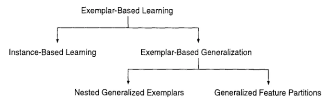
Figure 1. Classification of exemplar-based learning algorithms.

artificial datasets along with its comparison with other similar techniques are presented. The final section discusses the applicability of CFP and concludes with general remarks about the algorithm.

2. Exemplar-Based Models

Exemplar-based learning is a kind of concept learning methodology in which the concept definition is constructed from the examples themselves, using the same representation language. There are two main types of exemplar-based learning methodologies in the literature, namely instance-based learning and exemprar-based generalization (see Figure 1). Instance-based learning retains examples in memory as points in feature space and never changes their representation. However, in exemplar-based generalization techniques the point-storage model is slightly modified to support generalization.

An instance-based concept description includes a set of stored instances along with some information concerning their past performance during the training process. The similarity and classification functions determine how the set of saved instances in the concept description are used to predict values for the category attribute. Therefore, IBL concept descriptions contain these two functions along with the set of stored instances.

The instance-based learning technique (Aha et al., 1991) was first implemented in three different algorithms, namely IB1, IB2, and IB3. IB1 stores all the training instances, IB2 stores only the instances for which the prediction was wrong. Neither IB1 nor IB2 remove any instance from concept description after it had been stored. IB3 is the noise tolerant version of the IB2 algorithm. It employs a significance test to determine which instances are good classifiers and which ones are believed to be noisy. Later Aha (1992) implemented two extensions to these algorithms, called IB4, and IB5. IB4 learns a separate set of attribute weights for each concept, which are then used in the similarity function. IB5, which is an extension of IB4, can cope with novel attributes by updating an attribute's weight only when its value is known for both the instance being classified and the instance chosen to classify it.

IBL algorithms assume that instances which have high similarity values according to the similarity function have similar classifications. This leads to their local bias

(4)

50 H.A. GIJVENIR AND i. ~iRiN

for classifying novel instances according to their most similar neighbor's classification. They also assume that without prior knowledge attributes will have equal relevance for classification decisions (i.e., each feature has equal weight in the similarity function). This assumption may lead to significant performance degradation if the data set contains many irrelevant features.

In

Nested Generalized Exemplars

(NGE) theory, learning is accomplished by storing

objects in Euclidean n-space, E n, as hyperrectangles (Salzberg, 1991a). NGE adds generalization on top of the simple exemplar-based learning. It adopts the position that exemplars, once stored, should be generalized. The learner compares a new example to those it has seen before and finds the most similar, according to a similarity metric which is inversely related to the distance metric (Euclidean distance in n-space). The term

exemplar

(or

hyperrectangle)

is used to denote an example stored in memory. Over time, exemplars may be enlarged by generalization. This is similar to the generalizations of segments in the CFP algorithm. Once a theory moves from a symbolic space to Euclidean space, it becomes possible to

nest

one generalization inside the other. Its generalizations, which take the form of hyperrectangles in E ~, can be nested to an arbitrary depth, where inner rectangles act as

exceptions

to the outer ones.

EACH (Exemplar-Aided Constructor of Hyperrectangles) is a particular implementation of the NGE technique, where an exemplar is represented by a hyperrectangle. EACH uses numeric slots for feature values of every exemplar. The generalizations in EACH take the form of

hyperrectangles in Euclidean nrspace,

where the space is defined by the feature values for each example. Therefore, the generalization process simply replaces the slot values with more general values (i.e., replacing the range [a, b] with another range [c, d], where c < a and b < d). EACH compares the class of a new example with the most similar (shortest distance) exemplar in memory. The distance between an example and an exemplar is computed similarly to the

similarity

function of IBL algorithms, but exemplars and features also have weights in this computation and the result is the distance.

Wettschereck (1994) has recently implemented a hybrid k-nearest-neighbor (kNN) and batch nearest-hyperrectangle (BNGE) algorithm, called KBNGE. This hybrid system uses BNGE if in areas that clearly belong to one output class and kNN otherwise.

3. Learning with Feature Partitions

This section discusses a new incremental learning technique, based on

feature partition-

ing. The

description of CFP is presented first. The process of partitioning of a feature

dimension is illustrated by an example. An extension of CFP, called GA-CFR which uses genetic algorithms to determine a best setting of domain dependent parameters of CFP is also described. Finally, the limitations of CFP are discussed.

(5)

3.1. Basic Characteristics of CFP

In order to characterize the feature partitioning method, we will identify several properties of machine learning methods, and show how CFP differs from, or is similar to the others.

Knowledge Representation Schemes:

One of the most useful and interesting dimensions

in classifying machine learning (ML) methods is the way they represent the knowledge they acquire. Many systems acquire

rules,

which are often expressed in logical form, but also in other forms such as schemata. Other knowledge representation techniques include the use of a set of representative instances (Aha et al., 1991), hyperrectangles (Rendell, 1983; Salzberg, 1991a), and decision trees, as in ID3 (Quinlan, 1986a). Decision trees have low classification complexity and can be used in the implementation of very efficient classifiers. A monothetic 1 decision tree is global for each attribute, in other words, each non-leaf decision node may specify some test on any one of the attributes. On the other hand, in the CFP algorithm, a segment is the basic unit of representation. The CFP algorithm can be seen to produce a special kind of decision trees. While CFP considers projections of the whole problem space, ID3, when selecting the best attribute, only considers a subregion corresponding to the current path in the tree. Learning in CFP is accomplished by storing objects separately in each feature dimension as partitions of the set of values that it can take. Another important difference is that the classification performance of CFP does not depend critically on any small part of the model; in contrast, decision trees are much more susceptible to small alterations in the model (Quinlan, 1993).

Underlying Learning Strategies:

Most systems fall into one of two main categories

according to their learning strategies; namely,

incremental

and

non-incremental.

Systems that employ an incremental learning strategy attempt to improve an internal model (what- ever the representation is) with each example they process. However, systems employing non-incremental strategies must see all the training examples before constructing a model of the domain. Incremental learning strategies enable the integration of new knowledge with what is already known. The characteristic deficiency of these systems is that their performance is sensitive to the order of the instances (examples) they process. The CFP algorithm falls into the incremental learning category, which means that CFP's behavior is also sensitive to the order of examples.

Domain Independent Learning:

Some learning methodologies, e.g., explanation-based

learning (EBL), require considerable amounts of domain specific knowledge to construct explanations. Exemplar-based learning, on the other hand, incorporates new examples into its current experience by storing them verbatim in memory. Since it does not convert examples into a different representational form, an exemplar-based learning system does not need any domain knowledge to explain what conversions are legal, or even what the representation means. Interpretation is left to the user or domain experts. Consequently, exemplar-based systems like CFP can be quickly adapted to new domains, with a minimal amount of programming.

Multiple Concept Learning:

Machine learning methods have gradually increased the

number of concepts that they can learn and the number of variables they could process. Many early programs could learn exactly one concept from positive and negative in-

(6)

52 H.A. GUVENIR AND i. ~iRiN

stances of a concept. Most systems (e.g., CFP) that can handle multi-class concepts need to be told exactly how many classes they are to learn.

Type of Attribute Values: One shortcoming of many learning systems is that they

can handle only binary variables, or only continuous variables, but not both. Catlett (1991) presented a method for changing continuous-valued attributes into ordered discrete attributes for systems that can only use discrete attributes. The CFP algorithm handles variables which take on any number of values, from two (binary) to infinity (continuous). In general, CFP is most suitable for domains where feature values are linearly ordered, since generalization of segments is possible only on this type of values.

Problem Domain Characteristics: In addition to characterizing the dimensions along

which the CFP system offers advantages over similar methods, it is worthwhile to consider the sorts of problem domains it may or may not handle. Although CFP is domain independent, there are some domains in which the target concepts are very difficult for exemplar-based learning, and other learning techniques will perform better. In general, exemplar-based learning is best suited for domains in which the exemplars are clusters in feature space. The CFP algorithm, in particular, is applicable to concepts where each feature, independent of other features, can be used in the classification of the concept. If concept boundaries are nonrectangular, or projection of the concepts into a feature dimension overlap, the performance of CFP degrades.

Noise Tolerance: The ability to form a general concept description on the basis of

particular examples is an essential ingredient of intelligent behavior. If examples contain errors, the task of useful generalization becomes harder. The cause of these errors or "noise" may be either systematic or random. Noise, in general, can be classified as (1)

classification noise, and (2) attribute noise (Quinlan, 1986b; Angluin & Laird 1988).

Classification noise involves corruption of the class value, while attribute noise involves distortion of an attribute value of an instance. Missing attribute values are also treated as attribute noise.

Applicability of a learning algorithm depends highly on its capability for handling noisy instances (Lounis & Bisson, 1991). Therefore, most learning algorithms try to cope with noisy data. For example, the IB3 algorithm utilizes classification performance of stored instances to cope with noisy data. It removes instances from the concept description that are believed to be noisy (Aha et al., 1991). EACH also utilizes the classification performance of hyperrectangles. However, it does not remove any hyperrectangle from the concept description (Salzberg, 1991a). Decision tree algorithms utilize statistical measurements and tree pruning to cope with noisy data (Quinlan, 1986a; Quinlan, 1993). CFP utilizes representativeness values of segments, along with a voting scheme, to cope with noisy data. Unknown attribute values are simply ignored in CFR

3.2. The CFP Algorithm

This section describes the details of the feature partitioning algorithm used by CFE Learning in CFP is accomplished by storing the objects separately in each feature dimension as disjoint segments of values. A segment is the basic unit of representation in the CFP algorithm. Although it is not a requirement for CFR for the time being, let

(7)

CLASSIFICATION BY FEATURE PARTITIONING

53

,eel: <xl : Cl> ¶ee: <x~ : C1>

, " < [ x l , x l ] , C t , l > < [ x i , x 2 ] , C l , 2 > ,i Ixl- x21gDf

X I X 1 X 2

(a) (b)

e3:<x3 : C,>e *e4:<x4 : C2> [ X 2 - X 3 I _ Df { i < [ X4'[X4] 'C2'1> <[Xl, x3] ,C1,3> } <[Xl' X4] ,Cl,rI>i < [x4, x3],Cl,r2> --~iii[iiii~i~{ii{iiiiiiiiiiiN!i!i!i~i~iIIiiiiii~i{i{iiiIiiiiiiii{iii{i{iiiii~Niiii~ - f ~i{iiit!iiiiiiiii{iiiiiiiiiiiiiiiiii{iiiiiiiiiiiiiii[iiiiiiiii{iiiiiiN X l X 2 K 3 X 1 X4 X3 (c) (d) , f

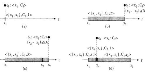
Figure 2. Partitioning of a feature dimension. Here, r 1 = 3 :ca-xl and r2 = 3 ~ .

:~3 ~Xl X3 --Xl

us assume that the set of values that a feature can take are linearly ordered. For each segment, lower and upper bounds of the feature values, the associated class, and the number of instances it represents are maintained. The class value of a segment may be

undetermined. An example (instance) is defined as a vector of feature values plus a label

that represents the class of the example.

Initially, a segment covers the entire range of the feature dimension, that is, ( ( - 0 % +Go),

undetermined, 0}. Here, the first element of the triple indicates the range of the segment

with lower and upper limits, the second its class, and the third, called the representa-

tiveness value, the number of examples represented by the segment. Suppose that the

first example el of class C1 is given during the training phase (Figure 2a). If the value of el for feature f is xl, that is eli = xl, then the set of possible values for feature f will be partitioned into three segments: ( ( - o o , xl]. undetermined, 0}, (Ix1, xl], C1, 1} and ([Xl, Go), undetermined, 0). A segment whose lower and upper limits are equal is called a point segment.

A segment can be extended through generalization with other neighboring points in the same feature dimension. The CFP algorithm pays attention to the disjointness of the segments to avoid over-generalization. In order to generalize a segment in feature f to cover a point, the distance between them must be less than a given generalization limit (Df). Otherwise, the new example is stored as another point (trivial) segment in the feature dimension f . Assume that the second example e2 (with x 1 < Z2) is close to el (i.e., Ixa -- x2l <_ D f ) in feature f and also belongs to the same class. In that case the CFP algorithm will generalize the segment for xl into an extended segment ([xl, x2], C1,2}, which now represents two examples (see Figure 2b). Generalization of a range segment is illustrated in Figure 2c.

If the feature value of a training example falls in a segment of the same class, then simply the representativeness value (number representing the examples in the segment) is incremented by one. On the other hand, if the new training example falls in a segment

(8)

54 H.A. GUVENIR AND i. ~tr~tN train(TrainingSet, A, D): begin foreach feature f, wf = 1 foreach e in TrainingSet foreaeh feature f if ef value is known if prediction_on_feature(f, e f) = ect~s then wf = (1 + A)wy else wf := (1 - A)wf

update - feature - partitioning(f, el, D y )

end

Figure 3. Training algorithm of CFR The process of updating a partition is described in the text.

with a different class than that of the example, CFP specializes the existing segment by dividing it into two sub-segments and inserting a point segment (corresponding to the new example) in between them (see Figure 2d). When a segment is divided into two segments, CFP distributes the representativeness of the old segment among the new ones in proportion to their sizes.

Segments may have common boundaries. If an example falls on a common boundary, the representativeness values of the segments are used to determine the predicted class value. For example, in Figure 2d at f = x4, two classes C1 and C2 are possible, but since the total representativeness of the class C1 is 3 and that of class C2 is 1, the prediction for the feature f is C1.

CFP does not apply generalization to nominal valued features. This is done by setting their generalization limit to zero. Therefore, the partition of a nominal feature is just a set of point segments.

The training process in the CFP algorithm has two steps: learning the feature weights and learning the feature partitions (Figure 3). The set of training instances, global weight adjustment rate (A), and the vector of generalization limits (D) are the arguments of the

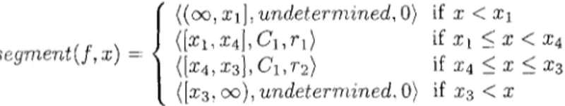
training procedure. For each training example, the prediction of each feature is compared with the actual class (eczass) of the example. The prediction_on_feature(f, ey) is

the class of the segment(f, el). The segment for a feature f and a value x, that is segment(f, x), is defined as the segment on feature f with the highest representativeness

value that includes the value x. For example, assuming that Ixa - z41 > Ix4 - xlt in Figure 2d,

{

( ( o % x l ] , u n d e t e r m i n e d , 0} if x < x l

s e g m e n t ( f , x) = ( [ x t , x4], C 1 , r l ) if x I ~ 27 < x 4

(Ix4, x3], C1, v2} if x4 _< x _< x3

([x3, oc), undeterr~ined. 0} if x3 < x

If the prediction on a feature f is correct, then the weight of that feature, w f is incre-

mented by w f . A, where A is a global feature weight adjustment rate; otherwise, it is

(9)

CLASSIFICATION BY FEATURE PARTITIONING 5 5

classification(e):

begin

foreach class c, votec = 0

foreach feature f

if e f value is known

c = prediction_on_feature(f, el)

if e ~ undetermined vo~ec = vOtec + w / return class c with highest voter.

end

Figure 4. Classification in CFP

The classification in CFP is based on a vote taken among the predictions made by each feature separately. For a given instance e, the prediction based on a feature f is determined by el, the value of e for feature f , as the class of s e g m e n t ( f , e l ) . The effect of the prediction of a feature in the voting is proportional to the weight of that feature. All feature weights are initialized to one before the training process begins. The predicted class of a given instance is the one which receives the highest amount of votes among all feature predictions. The classification algorithm of CFP is given in Figure 4. If the predictions of all the features are undetermined for a test instance, then the final prediction will be undetermined, as well.

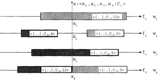
Figure 5 shows an example of the classification process of CFP on a domain with four features and two classes. Assume that the test example e has a class value C1 and features values are Xl, x2, x3, and x4, respectively. The prediction of the first feature is C1, that is it votes for class C1. The second feature predicts undetermined as a class value (abstention). The third feature votes for C2. The fourth feature value x4 of e falls into the border of two segments. In this case the representativeness values are used to determine the predicted class value. Since the segment of class C2 has a representativeness value of 12, which is greater than the representativeness of the segment of class CI, the prediction the fourth feature is C2. The final prediction of CFP depends on the votes of each feature and their weights (wi's). The class which receives the highest weight of votes is the predicted class. If wl > (w3 + 'w4) then CFP will classify e as a member of class C1 which is a correct prediction. Otherwise, it predicts the class of e as C~, which would be a wrong prediction.

The second step in the training process is to update the partitioning of each feature using the given training example. If the feature value of a training example falls in a segment of the same class, then its representativeness value is simply incremented. If the new feature value falls in a point segment of a different class to that of the example and it is a point segment, then a new point segment (corresponding to the new feature value) is inserted in addition to the old one. Otherwise, if the class of the segment is not undetermined, then the CFP algorithm specializes the existing segment by dividing it into two sub-segments and inserting a point segment (corresponding to the new feature value)

(10)

5 6 H.A. GOVENfR AND i. $iRtN

]

e

I , X 2 , x 3 , X 4 : C I >

'

<

x

i i

lliiiiii!i!i!iNiiiiiiiiiiiiiiiii!iNiNiiiiiNiNNiiiiN!Nii [

...

I

w

i i i iiiiii~ ... > l w m

Ix 2

[

"f2

i i i < [ . . ] , c 2 , 9 > | -~f3 w. b Ix3 i

o 2,

l

iiiiiii2[: ii 1 ; ; ; l

;

f

. . . , , - . . . 4 4 x 4

Figure 5. An example of classification in CFR Here, light gray refers to class C1 and dark gray to class C2.

between them. On the other hand, if the example falls into an undetermined segment, then the CFP algorithm tries to generalize the nearest segment of the same class with the new point. If the nearest segment to the left or right is closer than

Df

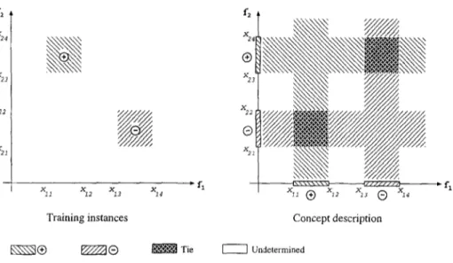
distance, and is of the same class as the training instance, than that segment is generalized to cover the training instance. Otherwise, a new point segment that corresponds to the new feature value is inserted.

In order to illustrate the form of the resulting concept descriptions learned by the CFP algorithm, consider a domain with two features f l and f2. Assume that during the training phase, positive ((9) instances with f l values in [Xlt, x12] and f2 values in [x23, x24], and negative ((9) instances with ft values in [x13, X14] and f2 values in [xzt, x22] are given. The resulting concept description is shown in Figure 6. This concept is represented in CFP by l0 segments (5 segments per feature) including the segments with undetermined class value. Note that these 10 segments implicitly represent 25 rectangles. In general,

n

CFP represents a concept in n-dimensional space using }-~f=l s(f), which implicitly represents rI~=l

s(f)

hyperrectangles, where

s(f)

represents the number of segments formed on feature f .

For test instances which fall into the region ( - o c , ,rll ) X [X23 , X24], for example, feature f l has no prediction, while feature ]:2 predicts class (9. Therefore, any instance falling in this region will be classified as (9. On the other hand, for instances falling into the region ( ( - o o , x l l ) , ( - o e , x21)), for example, the CFP algorithm does not commit itself to any prediction. For these instances the predicted class will be

undetermined.

If both features have equal weight (Wl = w2) then the description of the concept corresponding to the class (9 shown in Figure 6 can be written in 3-DNF as:

class O: (xtl _< f t & f l <_ X12 & f2 < X21) or (Xll --< f l & f l -< x12 & f2 > x22) or

(11)

CLASSIFICATION BY FEATURE PARTITIONING 57 f~ 5~ X23 52 5~ 5I 52 5., Training instances 5~ 5o ® 53 X22 ® %i I \ \ \ \ \ \ \ ' d p l l l / / l l , ' l Conceptdescription Tie [ - - I Undetermined , q

Figure 6. An example concept description in a domain with two features.

(z23 ~< f2 & f2 _< z24 & f l < 3713) or (3223 ~ f2 ~; f2 _< 3224 & f l > 3714) More compactly:

class 0: [(Zll ~< f l _< zd2) & (f2 < z21 or z22 < f2)] or

[(X23 ~ f2 -< Z24) • (fl < 3213 or xt 4 < f l ) ]

Since CFP uses a weighted majority voting, ties are broken in favor of the prediction of the feature with a higher weight. Continuing with the previous example, if 1/) 1 > 7JJ 2 then the ties will be broken in favor of f l during the voting process. In that case the concept description of the class ® will be as follows.

class 0: [xn _< f l _< xa2] or

[(z23 ~< f2 _< z24) & (fl < z13 or Z14 • fl)]

CFP does not assign any classification to an instance if it could not determine the appropriate class value for that instance. This may occur if the prediction on each feature is undetermined. In this case, CFP returns undetermined as the classification.

Note that point segments formed by splitting existing range segments with known class values remain as point segments, regardless of how close they are to other same class point segments. This type of fragmentation can be prevented by keeping the generalization limit low. On the other hand, keeping the generalization limit too low precludes the formation of pure range segments. This situation occurs especially in noisy domains. However, the use of the representativeness values in determining the

(12)

58 H.A. GOVENiR A N D I. ~tRIN

predictions on features reduces the effects of these point segments. This type of implicit pruning of point segments helps CFP avoid over-fitting the training data.

The CFP algorithm, in its current implementation, is a

categorical

classifier, since it returns a unique class for a given query (Kononenko & Bratko, 1991). Although we have not implemented it, it is possible to assign levels of confidence to decisions. The level of confidence for a decision can be computed by simply normalizing the votes that each class receives, as

VOtec

~ k votek

where c is the class assigned to a query. In that case, CFP returns a probability distribution over all classes, as in ASSISTANT (Cestnik et al., 1987).

3.3. Learning the Domain Dependent Parameters for CFP

Learning the domain dependent parameters for CFP can be seen as a parameter optimization problem. The goal is to determine the values of the domain dependent parameters that maximize the accuracy of the CFP algorithm. Genetic algorithms (GA) have been used successfully in parameter optimization tasks. For example, the GA-WKNN algorithm (Kelly & Davis, 1991) combines the optimization capabilities of a genetic algorithm with the classification capabilities of the WKNN

(weighted k nearest neighbor)

algorithm. The goal of the GA-WKNN algorithm is to learn an attribute weight vector that improves the WKNN classification performance. Chromosomes are vectors of real-valued weights. Following the same approach we developed the GA-CFP tool which is a hybrid system that combines a genetic algorithm with CFR The GA-CFP determines a setting of the domain dependent parameters for CFP which maximizes the accuracy (Gfivenir & ~irin,

1993a).

A chromosome in GA-CFP is a vector of real values representing the domain dependent parameters of CFP, i.e., A and

Df

for each feature. Therefore, the length of the chromosome is equal to the number of features plus one. GA-CFP employs the standard operators of genetic algorithms, namely reproduction, crossover and mutation, along with the elitist approach, where the best chromosome is always copied to the next genera- tion (Goldberg, 1989). GA-CFP uses uniform crossover, where two alleles of a pair of chromosomes undergoing the crossover operation are swapped with probability of 0~5. Mutation on an allele is obtained by multiplying its value by a random number from [0.5,1.5].

In setting the initial population for the genetic algorithm, the A values are randomly selected from the set [0, 0.1]. The initial

D z

values for linear type attributes are randomly selected from the set [0.05.range(f),

O.

15.

range(f)],

where

range(f )

is the difference between the maximum and minimum values for feature f . The

Df

values for nominal attributes are set to zero, and remain zero through the genetic operators.

As the fitness function for the genetic algorithm, GA-CFP uses two-fold cross-validation accuracy of the CFP on the training set with the parameters encoded in a chromosome.

(13)

C L A S S I F I C A T I O N BY F E A T U R E P A R T I T I O N I N G 59 f2

/

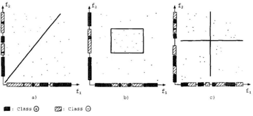
- y / / / / / ~ / / f-1 a) m : Class @ f~ fl b) 22g: class @ ff~ fl c)

Figure 7. Domains where projections of concepts into a feature dimension are overlapping.

Although it is possible to use the leave-one-out accuracy as the fitness value, our experimental results indicate that two-fold cross-validation accuracy gives a good approximation to determine the best settings of the domain dependent parameters.

3.4. Limitations of CFP

Classification in CFP is based on a weighted voting among individual predictions performed on each feature using only their local knowledge. Therefore, CFP is best applicable to concepts where each feature, independent of other features, can contribute to the classification of the concept. However, as is shown in the rest of this section, CFP is robust and performs reasonably well even in many domains that do not have this property.

The CFP algorithm has been tested on the three artificially generated two-dimensional domains shown in Figure 7. In each domain, data set contains equal number of instances of two classes, represented by @ and @.

Each segment represents two (one, if lower and upper values of the segment are equal) parallel surfaces (hyperplanes) in the description space; these are orthogonal to the axis of the segment and parallel to all other axes. Consequently, the regions constructed by CFP are disjoint hyperrectangles, except for their boundaries. When actual class regions are not hyperrectangles, the best that CFP can do is to approximate the regions by small hyperrectangles. This situation is illustrated in Figure 7a. The feature weights are learned as wl = 1.1494 and ws = 1.0822. Since the instances are symmetrically distributed in the feature space, the weights of the features are close to each other as expected, Segments for higher values of fl are labeled as class @, while segments for higher values of f2 are labeled as class @. Therefore, for higher values of fl class @ will be predicted, whereas for higher values of A class @ will be predicted. However, since w'l is slightly more than w2, few of the @ class instances near the border might be classified as @ mistakenl,/.

(14)

60 H.A. GIJVENIR AND I. ~itttN

If the projections of concepts on feature dimensions do not overlap, then CFP will classify an instance with a high confidence. However, in some circumstances, e.g., in nested concept descriptions, this may not hold. This case is illustrated in Figure 7b. The feature weights are determined by CFP as Wl = 1.0607 and w2 = 1.0512. The projections of the rectangle on the axes are represented mostly by O segments, while the remaining portions are represented by only ® segments. Therefore, all instances falling outside of the rectangle will be classified correctly, while instances falling into the rectangle will be correctly identified only with high confidence. Only a few of the instances in the rectangle will be misclassified.

In some cases, even when concepts descriptions are not nested, the projection of the concept descriptions may overlap, as shown in Figure 7c. The feature weights are determined by CFP as wl = 1.0186 and w2 = 1.0190. In this domain the instances are evenly distributed in the feature space and the weights of the features are close to each other as expected. Therefore, only this domain represents a difficult concept for CFP to learn.

There are two aspects of the CFP algorithm which may be considered as limitations. If two or more segments share a common point, then the classification predicted at the boundary is simply the segment with the largest number of representatives. Although it helps to override a point segment caused by a noisy training instance, it also implies that a legitimate point segment (say of class C1), formed by splitting a large segment (say of class C2), will not be able to classify future examples correctly until the number of future instances of the former class (C1) is sufficiently large.

The second aspect is that once a large segment is formed there is no way to generalize the point segments that fall in that segment. In order to avoid over-generalized segments we keep the generalization limits as small as possible, but large enough to form homogeneous segments.

4. Evaluation of CFP

A theoretical analysis of the CFP algorithm with respect to PAC-learning theory (Valiant, 1994) is given in (Gtivenir & ~irin, 1993b). It is clear that for n features and m training instances CFP generates at most

mn

segments (for

D]

= 0). Since the search for the prediction on a feature can take at most log m steps (using a binary search) on the average, the classification time complexity of the CFP algorithm is

O(n

log m). The training time complexity can be shown to be

O(mnlogm).

However, in this implementation of the CFP algorithm, we used linear search due to its simplicity. Therefore, this implementation has

O(nm)

classification 2 and O(r~m 2) training complexity.

The rest of this section presents an empirical analysis of the CFP algorithm. We tested the CFP algorithm on some of the datasets that are publically available in the UCI repository, and compared its accuracy with two other basic classification algorithms. In order to evaluate the robustness of the algorithm in the presence of irrelevant attributes we also tested it on artificially generated data.

(15)

4.1. Evaluation of CFP on Real-World Data

This section presents the experimental results of the CFP algorithm on some of the widely used real-world datasets from the UCI repository. The use of real-world data in these tests provided a measure of the system's accuracy on noisy and incomplete datasets, and also allowed comparisons between CFP and other similar systems.

From the viewpoint of empirical research, one of the main difficulties in comparing various algorithms which learn from examples is the lack of a formally specified model on which the algorithms may be evaluated. Typically, different learning algorithms and theories are given together with examples of their performance, hut without a precise definition of learnability it is difficult to characterize the scope of the applicability of an algorithm or to analyze the success of different approaches and techniques. Recently, there have been attempts to devise empirical evaluation criteria for comparing classifiers' performance (e.g, Kononenko & Bratko, 1991; Weiss & Kapouleas, 1989). Since CFP is more suitable to domains where the attribute values are linearly ordered, we chose to test it on the datasets that have this property, instead of a general benchmark set as given by Zheng (1993). We chose to test the CFP algorithm on the following datasets that have numerical attributes from the UCI repository: Breast cancer (Wisconsin), Cleveland, Diabetes, Glass, Horse-colic, Hungarian, Ionosphere, Iris, Musk and Wine.

The Breast cancer (Wisconcin) dataset contains nine numeric valued features; there are 16 missing attribute values. The Cleveland and Hungarian datasets are described by 13 features, 5 of which take linear values. Both of these datasets contain missing attribute values. The Pima Indians Diabetes dataset contains eight numeric valued features, with no missing values. The Glass dataset has nine attributes, all of which are continuous; there are no missing attribute values. The Horse colic dataset has 22 features (features V3, V25, V26, V27, and V28 are deleted from the original dataset). Seven of these features take continuous values. About 30% of the attribute values are missing. Attribute V24 is used as the class. The Ionosphere dataset contains 34 continuous features, with no missing values. The Iris Flowers dataset consists of four integer valued attributes, with no missing values. The Musk (cleanl) dataset has 166 linear valued features, with no missing values. The Wine dataset contains thirteen attributes all of which take continuous values, without any missing attribute values.

We compared CFP with two other classification algorithms that consider each feature separately, viz, the Naive Bayesian Classifier (NBC) and the Nearest Neighbor on Feature

Projections (NNFP) classifiers. Here, NBC is the Bayes classifier with the assumption

that the attributes are independent (Duda & Hart, 1973). This method is well known and will not be discussed in detail. We have implemented a new version of the NN (kNN, with k=l) classifier to be used for comparisons with CFR Similar to the CFP algorithm, the NNFP classifier considers each feature separately. Given a test instance, for each feature, it selects the training instance whose projection on that feature is the nearest. The prediction of a feature is the class of the nearest neighbor for that feature. Then, the class of a test instance is predicted through a vote among the individual predictions of the features. The features with missing values are simply ignored, as in CFR Each

(16)

62

H . A G I J V E N I R AND [. $IRtN 100,0 e ~ r , o~ o= o ~5 99.0 98.0 97.0 96.0 95.0 94.0 93.0 92.0 91.0 90.0

/

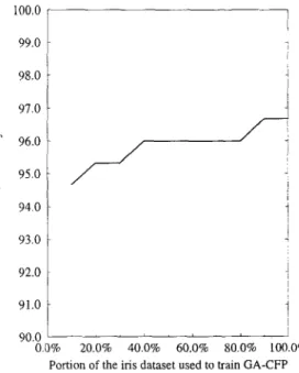
0.0% 20.0% 40.0% 60.0% 80.0% 100.0% Portion of the iris dataset used to train GA-CFP

Figure 8. A good setting of domain dependent parameters can be learned by GA-CFP using a small portion

of the dataset.

feature has the same weight in the voting. Therefore, the prediction for a query is the class that occurs most often in this set of individual feature predictions.

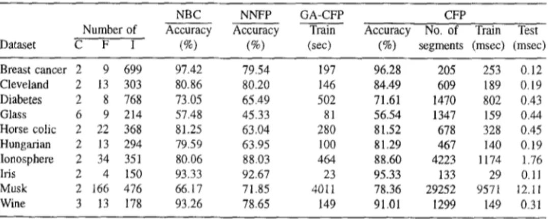
The empirical comparisons of CFP with NBC and NNFP are shown in Table 1. In these comparisons we used leave-one-out cross-validation, which involves removing exactly one example from the data and training the algorithm on the remaining examples and measuring the accuracy by using that single instance as the test instance. The test is repeated for every example in the dataset and accuracy is measured as the average accuracy across all examples. Each training time given below is the average time to train CFP with a number of instances one less than the data size. The testing time is the average time to classify the single test instance.

In these experiments the values of the domain dependent parameters for the CFP algorithm were determined with the help of the GA-CFP program. For each dataset the GA-CFP was trained with a dataset comprising only a randomly selected 20% of the instances from the actual dataset.

We have observed that the portion of the training data used by the GA-CFP did not have much effect on the leave-one-out classification accuracy of the CFP with the resulting domain dependent parameters. This fact is illustrated on the iris domain in Figure 8. As shown in this graph, the accuracy obtained by CFP with the parameters learned by GA-CFP using only 20% of the data is only 1.33 points below the case where 100% of the data used.

The fitness value of a chromosome is the two-fold cross-validation accuracy of CFP on that training dataset. The population size was 100. In these experiments, the probability of crossover was 0.7 and the probability of mutation was 0.1. The domain dependent pa-

(17)

63

Table l. Comparison of leave-one-out cross-validation accuracy (%) of CFR NBC and NNFP on several real-

world data.sets. Training and testing times of CFP on these datasets are also given to indicate their dependence

on the number of features, instances and segments. Note C: Classes, F: Features, I: Instances.

NBC N N F P GA-CFP CFP

Number of Accuracy Accuracy Train

Dataset C F I (%) (%) (sec)

Accuracy No. of Train Test

(%) segments (msec) (msec)

Breast cancer 2 9 699 97.42 79.54 197 96.28 205 253 0.12 Cleveland 2 13 303 80.86 80.20 146 84.49 609 189 0.19 Diabetes 2 8 768 73.05 65.49 502 71.61 1470 802 0.43 Glass 6 9 214 57.48 45.33 81 56.54 1347 159 0.44 Horse colic 2 22 368 81.25 63.04 280 8152 678 328 0.45 Hungarian 2 13 294 79.59 63.95 100 81.29 467 140 0.19 Ionosphere 2 34 351 80.06 88.03 464 88.60 4223 1174 1.76 Iris 2 4 150 93.33 92.67 23 95.33 133 29 0.11 Musk 2 166 476 66.17 71.85 4011 78.36 2 9 2 5 2 957t 12.11 Wine 3 13 178 93.26 78.65 149 91.01 1299 149 0.31

rameters represented by the chromosome with the highest fitness value in 50 generations were used by CFP to measure the leave-one-out classification accuracy.

The comparison of leave-one-out cross-validation accuracies of CFP with NBC and N N F P are given in Table 1. Measured training (with all dataset except one instance) and testing times (with a single test instance) for leave-one-out cross-validation of C F P on these datasets are also given to indicate their dependence on the number o f features, instances and total number of segments formed on all features after training. As seen in this table, the training time is approximately proportional to the product of number of features and the square of number of instances. Also the classification (testing) time is proportional to the product of the number o f features and number o f segments.

These results indicate that the C F P algorithm is competitive with the two alternative algorithms on standard datasets where most of the features take continuous values. Holte (1993) has implemented a simple classifier, called 1R (for 1 rules), that classifies an instance on the basis o f a single attribute, independent of other attributes. In this respect, CFP also produces a single rule for each feature, but applies a weighted voting scheme among these rules to determine the final classification. Holte has pointed out that the most datasets in the UCI repository are such that, for classification, their attributes can be considered independently o f each other, which explains the success o f the CFP algorithm on these datasets.

4.2. Evaluation o f C F P on Irrelevant Attributes

In many practical applications, it is often not known exactly which input attributes are relevant. The natural response of users is to include all attributes that they believe could possibly be relevant and let the learning algorithm determine which features are in fact worthwhile.

(18)

64 H.A. GISVENIR AND I. 8IRtN >. < 98 i 95 i 94 i 93 i 92 ! 91 90 L . . . 0 I 2 3 4 5 6 7 8 9 10 N u m b e r of irrelevant attributes 4 0 ~ r - - 3500 ' 3O0O i 2500 1000 500 0 1 2 3 4 5 6 7 8 9 10 N u m b e r o f irrelevant attributes 1000 L

8°;

/

400 7 200 ~ 0 3 i U

[

i l . f 0 I 2 3 4 5 6 7 8 9 10 I 2 3 4 5 6 7 8 9 10

N u m b e r of irrelevant attributes N u m b e r of irrelevant attributes

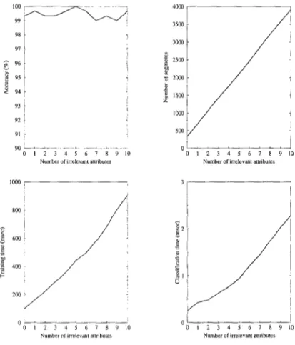
Figure 9. Accuracy, memory requirements, training and testing times of CFP on increasing number of irrelevant attributes.

In order to assess the robustness of the CFP against irrelevant attributes in the domain, we have performed an experiment on an artificially generated datasets. In this experiment we defined three classes as hyperrectangles over four dimensions; they were [0, 5] x [0, 2] × [0, 2] × [0, 0], [4, 6] × [4, 8] × [5, 7] × [4, 6] and [7, 101 x [7, 10] × [2, 4] × [2, 4.5]. That is, the concepts have similar shape to the one shown in Figure 7b. The dataset contained 100 instances of each class, where attributes take on values from the set [0,10]. We have performed eleven experiments, in each of which we added an extra irrelevant attribute with randomly generated values. The first experiment does not contain any irrelevant attribute, while the last experiment contains ten irrelevant attributes (fourteen attributes in total). The results of these experiments are shown in Figure 9. The results given in this figure are average of leave-one-out tests. The training time is the time required to train with 299 instances, while the testing time is the time to classify a test instance.

In these experiments the A was set to 0.05 and the generalization limits were 1.0 for each attribute. As shown in Figure 9, the accuracy of the CFP algorithm is independent of the number of attributes in the dataset. However, the total number of segments

(19)

constructed increases linearly with the number of irrelevant attributes, since the number of segments in each irrelevant attribute is roughly equal to the number of instances. Since we used simple linear search on each feature partition for classification, the training and testing times are linearly proportional to the total number of segments. The total number of segments on four relevant attributes is 338 on the average, while for fourteen attributes it is 3990. Also in these experiments the weights of the relevant attributes are found to be more than 100, while the weights of the irrelevant attributes are less than 0.1. These experiments show that the CFP algorithm is robust against irrelevant attributes in a domain.

5. Conclusion

In this paper we have presented a new exemplar-based generalization method of learning based on feature partitioning, called CFP. It is an inductive, incremental and supervised learning method. CFP learns a partitioning of values for each feature of the application domain. The CFP algorithm is applicable to domains where each feature, independent of other features, can be used to classify the instances. CFP makes significant modifica- tions to the exemplar-based learning algorithms. It treats feature values independently, allowing their generalization in the form of feature segments.

This approach is a variant of algorithms that learn by projecting into one feature dimension at a time. The novelty of CFP is that it retains a feature-by-feature representation and uses a voting scheme in categorization. CFP learns by projecting into one feature dimension at a time. Therefore, it loses the n-dimensional information of the description space. This weakness is compensated with a weighted voting scheme.

Another important improvement is the natural handling of unknown attribute values. Most inductive learning systems use ad hoc methods for handling unknown attribute values. Since the value of each attribute is handled separately, attributes with unknown values are simply ignored by CFP.

CFP will clearly fail in some cases. For example, if the projections of concepts on an axis overlap each other, the CFP constructs many segments of different classes next to each other. In that case, the accuracy of classification depends on the observed frequency of the concepts.

CFP uses feature weights to cope with irrelevant attributes. Introducing feature weights protects the algorithm's performance when an application domain has irrelevant attributes. The feature weights are dynamically adjusted according to the global weight adjustment rate (A), which is an important parameter for the predictive accuracy of the algorithm. Another important component of CFP is the generalization limit for each attribute, which controls the generalization process.

The use of feature weights enables the CFP algorithm to cope with the irrelevant attributes that may exist in the dataset. Existence of irrelevant attributes do not affect the accuracy of the algorithm. However the memory requirements and training and classification times linearly increase with the number of irrelevant attributes.

The weight adjustment rate and generalization limits are domain dependent parameters of CFR and their selection affects the performance of the algorithm. Determining the

(20)

66

H.A. G I J V E N i R A N D i. ~ i R i N

best values for these parameters is an optimization problem for a given domain. In GA- CFP a genetic algorithm is used to find a good setting of these parameters. The GA-CFP is a hybrid system, which combines the optimization capability of genetic algorithms with classification capability of the CFP algorithm. The genetic algorithm is used to determine the domain dependent parameters for CFP, that is, weight adjustment rate and generalization limits. Then, the CFP algorithm can be used with settings that are learned by the genetic algorithm.

A segment is the basic unit of representation in the CFP algorithm. Each segment represents a region between two parallel surfaces (hyperplanes) in feature space, that are orthogonal to the axis of the segment and parallel to all other axes. Consequently, the regions constructed by CFP are disjoint hyperrectangles. Since CFP retains a feature- by-feature representation, projection of concepts will determine the applicability of the CFP to a given domain. CFP is not applicable to domains where all of the concept projections overlap, or domains in which concept descriptions are nested. In other words, CFP is applicable to domains where each feature can contribute to the classification independently of others. This claim has been supported by an empirical evaluation of the CFP algorithm on commonly used datasets that have continuous feature values.

Acknowledgments

We would like to thank our editor, Ross Quinlan, and our anonymous reviewers. Their insightful suggestions resulted in a substantially improved article. Special thanks to D. Aha for his helpful comments on the earlier drafts of the paper. We thank Tom Mitchell for a discussion on the applicability and evaluation of this technique. We also gratefully acknowledge EM. Murphy and D. Aha for creating and managing UCI Repository of machine learning databases. The breast cancer dataset was provided by Dr, William H. Wolberg from the University of Wisconsin Hospitals.

Notes

1. Polythetic decision trees can use more than one attribute in the tests at their internal nodes.

2. The classification time is cc • n s/rz = cc • s, where cc is a constant, and s < m - n is the total number of segments.

References

Aha, D.W. (1992). Tolerating noisy, irrelevant and novel attributes in instance-based learning algorithms. Int. J. Man-Machine Studies, 36, 267-287.

Aha, D.W., Kibler, D. & Albert, M K . (1991). Instance-based learning algorithms. Machine Learning, 6,

37~66.

Angluin, D. & Laird, E (1988). Learning from Noisy Examples. Machine Learning, 2, 343-370.

Catlett, ]. (1991). On changing continuous attributes into ordered discrete attributes. In Y. Kodratoff (Ed.)

(21)

67

Cestnik, B., Kononenko, I, & Bratko, I. (1987). ASSISTANT 86: A Knowledge elicitation tool for sophisticated users. In 1. Bratko, N. Lavrac (Eds.), Progress in machine learning. Wilmslow, England: Sigma Press.

Cost, S, & Salzberg, S. (1993) A weighted nearest neighbor algorithm for learning with symbolic features,

Machine Learning, 10, 57-78.

Duda, R.O. & Hart, P.E. (1973). Pattern Classification and Scene Analysis. New York: Wiley & Sons.

Goldberg, D.E. (1989). Genetic algorithms in search, optimization, and machine learning. Marylandi Addison-

Wesley.

Giivenir, H.A. & ~irin, I. (1993a). A genetic algorithm for classification by feature partitioning. Proceedings of the Fifth International Conference on Genetic Algorithms (pp 543-548). Urhana-Champaign, IL: Morgan

Kaufmann.

Giivenir, H.A. & ~irin, I. (1993b). The complexity of the CFE a method for classification based on feature partitioning. In E Torasso (Ed.) Advances in Artificial Intelligence, Lecture Notes in Artificial Intelligence, LNAI 728. (pp. 202-207). Berlin: Springer-Verlag.

Holte, R. C. (1993). Very simple classifcation rules perform well on most commonly used datasets. Machine Learning, 11, 63-91.

Kelly, J.D. & Davis, L. (1991). A hybrid genetic algorithm for classification. Proceedings of the Twelfth Inter- national Joint Conference on Artificial Intelligence. (pp. 645-650). Sydney, Australia: Morgan Kaufmann.

Kononenko, I. & Bratko, I. (1991). Information-Based Evaluation Criterion for Classifier's Performance.

Machine Learning, 6, 67-80.

Lounis, H. & Bisson, G. (1991). Evaluation of learning systems: An artificial data-based approach. In Y. Kodratoff (Ed.) Machine Learning-EWSL-91 (pp. 463-481). Springer-Verlag.

Medin, D.L. & Schaffer, M.M. (1978). Context theory of classification learning. Psychological Review, 85,

207-238.

Quinlan, J.R, (1986a). Induction of decision trees. Machine Learning, 1, 81-106.

Quinlan, J.R. (1986b). The effect of noise on concept learning. In RS. Michalski, J.G. Carbonell, & TM. Mitchell (Eds.), Machine learning: An artificial intelligence approach (Vol. II). San Mateo, CA:

Morgan Kaufmann.

Quinlan, J.R. (1993). C4.5: Programs for machine learning. San Mateo, CA: Morgan Kaufmann.

Rendell, L. (1983). A new basis for state-space learning systems and successful implementation. Artificial Intelligence, 20, 369-392.

Salzberg, S. (1991a). A nearest hyperrectangle learning method. Machine Learning, 6, 251-276.

Salzberg, S. (1991b). Distance metrics for instance-based learning. Proceedings of the Sixth International Symposium on Methodologies fbr Intelligent Systems (pp. 399-408). Charlotte, NC.

Stanfill, C., & Waltz, D. (1986). Toward memory-based reasoning. Communications of the Association for Computing Machinery, 29, 1213-1228.

Valiant, L.G. (1984). A theory of the learnable. Communications of the A CM, 27, 1134-1142.

Weiss, S.M. & Kopoaleas I. (1989). An Empirical Comparison of Pattern Recognition, Neural Nets, and Machine Learning Classification Methods. Proceedings of the Eleventh International Joint Conference on Artificial Intelligence (pp. 781-787). Sam Mateo, CA: Morgan Kaufmann.

Wettschereck, D. (1994). A hybrid nearest-neighbor and nearest-hyperrectangle algorithm, Proceedings of the European Conference on Machine Learning (pp. 323-335). Catania, Italy: Springer-Verlag.

Zhang, J. (1992). Selecting typical instances in instance-based learning Proceedings of the Ninth International Machine Learning Conference (pp. 470-479). Aberdeen, Scotland: Morgan Kaufmann.

Zheng, Z. (1993). A Benchmark for Classifier Learning. Proceedings of the 6th Australian Joint Conference on Artificial Intelligence (pp. 281-286). Melbourne, Australia: World Scientific.

Received August 9, 1994 Accepted May 4, 1995 Final Manuscript July 27, 1995