MODELING AND OPTIMIZATION OF CENTRAL RING
TRANSPORTATION SYSTEM (CRTS) IN TURKISH
LAND FORCES
A THESIS
SUBMITTED TO THE DEPARTMENT OF INDUSTRIAL ENGINEERING
AND THE INSTITUTE OF ENGINEERING AND SCIENCES OF BILKENT UNIVERSITY
IN PARTIAL FULFILMENT OF THE REQUIREMENTS FOR THE DEGREE OF
MASTER OF SCIENCE
By
Hamdi Ünal Akmeşe JULY,2003
I certify that I have read this thesis and in my opinion it is fully adequate, in scope and in quality, as a thesis for the degree of Master of Sciences.
Assoc.Prof. Osman Oğuz (Principal Advisor)
I certify that I have read this thesis and in my opinion it is fully adequate, in scope and in quality, as a thesis for the degree of Master of Sciences.
Assoc.Prof. Mustafa Pınar
I certify that I have read this thesis and in my opinion it is fully adequate, in scope and in quality, as a thesis for the degree of Master of Sciences.
Asst.Prof. Oya Ekin Karaşan
Approved for the Institute of Engineering and Sciences
Prof. Mehmet Baray
ABSTRACT
MODELING AND OPTIMIZATION OF CENTRAL RING
TRANSPORTATION SYSTEM (CRTS) IN TURKISH LAND
FORCES
Hamdi Ünal Akmeşe
M.S. in Industrial Engineering
Advisor:Assoc. Prof. Osman Oğuz
July 2003
This thesis shows how Turkish Land Forces can optimally meet delivery and pick-up demands of its units via Central Ring Transportation System. A mixed integer programming model is proposed, and for the implementation of the model, mathematical modeling software GAMS is used. The model is implemented for three different fleet sizes of vehicles (4-vehicle, 5-vehicle, 6-vehicle) with taking eight-week data of 2002 into account. How transportation costs are affected by the number of vehicles is investigated, and an ideal number of vehicles and the optimal routes to be followed are proposed.
Keywords : Mixed Integer Programming, Capacitated Vehicle Routing, Time Windows, Transportation Costs.
ÖZET
KARA KUVVETLERİ MERKEZİ RİNG TAŞIMACILIĞI
SİSTEMİNİN MODELLENMESİ VE OPTİMİZASYONU
Hamdi Ünal Akmeşe
Endüstri Mühendisliği Bölümü Yüksek Lisans
Tez Yöneticisi: Doç. Dr. Osman Oğuz
Temmuz 2003
Bu çalışma Türk Kara Kuvvetlerinin kendi birliklerinin sevkiyat ve toplama taleplerini Merkezi Ring Taşımacılığı Sistemi vasıtası ile en uygun olarak nasıl karşılayabileceğini göstermektedir. Bunun için tamsayılı programlama modeli önerilmiş ve bu modelin uygulanması için matematiksel modelleme yazılımı GAMS kullanılmıştır. 2002 yılına ait sekiz haftalık bilgier gözönüne alınarak, model üç farklı sayıdaki araç filoları (4-araç, 5-araç, 6-araç) için çalıştırılmıştır. Taşıma maliyetlerinin araç sayısına bağlı olarak nasıl etkilendiği sorusuna yanıt bulunmaya çalışılmış ve ideal araç sayisi ile bunlarin izleyeceği ideal rotalar önerilmiştir.
Anahtar Kelimeler : Tamsayılı Programlama, Kapasite Sınırlı Araç Güzergahı Bulma, Zaman Kısıtları, Taşıma Maliyetleri.
ACKNOWLEDGEMENT
I would like to express my gratitude to Assoc.Prof. Osman Oğuz for his guidance, attention, interest and patience throughout our study.
I am indebted to the readers Assoc. Prof. Mustafa Pınar and Asst.Prof. Oya Ekin Karaşan for their effort, kindness and time.
I would like to thank Captain Ümit Ata Narin for his support to attend a MS program, guidance and understanding during the years in Bolu.
I am very thankful to Savas Çevik,Ömer Selvi, Güneş Erdoğan, Çağatay Kepek, Halil Şekerci, Duygu Pekbey for their assistance, support and friendship during the graduate study. I am also indebted to all Industrial Engineering Dept. staff.
I am grateful to Turkish Land Forces for giving the opportunity to continue my education in Bilkent University.
CONTENTS
List of Figures
X
List of Tables XI
English-Turkish Meanings of Some Military Terms
XII
1.INTRODUCTION
1
1.1. Central Ring Transportation System (CRTS) 2
1.1.1. Provision Types of Land Forces 2
1.1.2. Current and Proposed CRTS 3
2. LITERATURE REVIEW
7
2.1. The TSP and m-TSP
7
2.1.1. Mathematical Formulations of m-TSP 8 2.1.2. Solution Methods for m-TSP 102.1.2.1.Exact Solution Methods for m-TSP 11
2.1.2.2.Heuristic Solution Methods for m-TSP 12
2.1.2.2.1.Tour Construction Heuristics 12
2.1.2.2.2.Tour Improvement Heuristics 13
2.1.2.3.Transformation to TSP 15
2.2.Vehicle Routing Problems (VRP)
15
2.2.1. Mathematical Formulations of VRP 16
2.2.2. Solution Methods for VRP 21
2.2.2.1.Exact Solution Methods for VRP 22
2.2.2.2.Heuristic Solution Methods for VRP 25
3.ANALYSIS OF THE PROBLEM and MATHEMATICAL
FORMULATION
29
3.1. Data File 29
3.1.1.Main Depot and Garage 293.1.2. Points 30
3.1.3. Vehicles 30
3.1.4. Items 31
3.2. Assumptions
32
3.2.1. All Demands Must be Satisfied 32 3.2.2. All Demands are Fixed and Known in Advance 32 3.2.3. The Load/Unload Times are Fixed and Known in Advance 33 3.2.4. Time Windows are Fixed and Known in Advance 33 3.2.5. Vehicle Speed is Fixed and Known in Advance 33 3.2.6. The Number of Vehicle is Fixed and Known in Advance 33
3.3.
Formulation 34
3.3.1. Indices 34
3.3.2. Initial Data and Parameters 34
3.3.3. Variables
35
3.3.4. Constraints
35
3.3.4.1. Assignment Constraints
35
3.3.4.2. Capacity Constraints
36
3.3.4.3. Load Feasibility Constraints
36
3.3.4.4. Time Feasibility Constraints
37
3.3.4.5. Non-Negativeness and Binary Variables
37
3.3.5. Objective Function
38
3.4. Experimentation
39
3.5. Results
41
3.5.1. Case 1: Fleets of Five Vehicles are Employed 42 3.5.2. Case 2: Fleets of Four Vehicles are Employed 43 3.5.3. Case 3: Fleets of Six Vehicles are Employed 444.CONCLUSION 48
4.1. Future Research Topics
49
Bibliography 50
Appendix 57
A. Data File 57
List of Figures
Figure 1.1. Routes of the Current System. 4 Figure 1.2. Routes of Sample Problem Solved by Proposed Model. 5
Figure 2.1. Crossover. 27
Figure 2.2. Customer Relocation. 27
Figure 2.3. Customer Exchange. 27
Figure 2.4. Transformation to Four Depots. 28 Figure 3.1. Comparison of The Current System with The Proposed
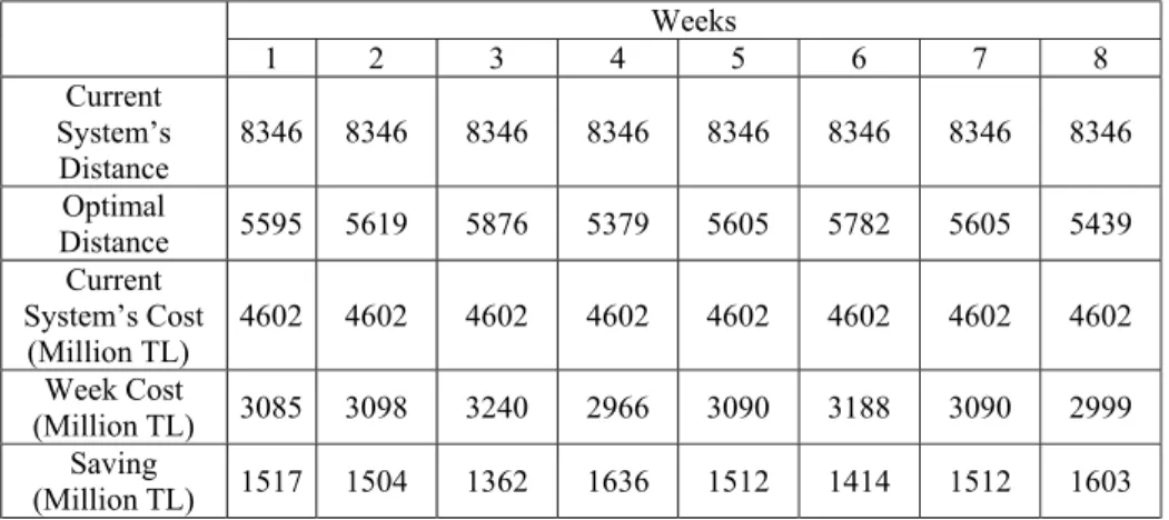
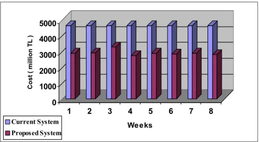
System in Distance for Weeks in Case 1. 42 Figure 3.2. Comparison of The Current System with The Proposed
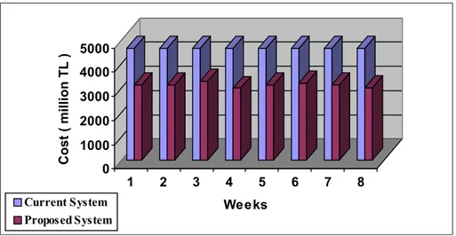
System in Cost for Weeks in Case 1. 43 Figure 3.3. Comparison of The Current System with The Proposed
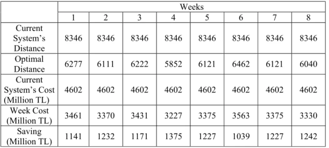
System in Distance for Weeks in Case 2. 44 Figure 3.4. Comparison of The Current System with The Proposed
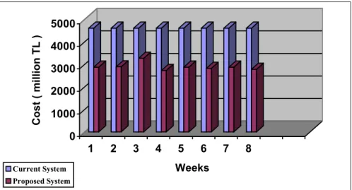
System in Cost for Weeks in Case 2. 45 Figure 3.5. Comparison of The Current System with The Proposed
System in Distance for Weeks in Case 3. 46 Figure 3.6. Comparison of The Current System with The Proposed
System in Cost for Weeks in Case 3. 46 Figure 3.7. Comparison of Cases in Distance for Weeks 46
List of Tables
Table 1.1. Demanding Points of the Sample Problem. 5 Table 3.1. Capacities of The Vehicles 31 Table 3.2. Required CPU Times, Number of Iterations and Number of
Nodes When Five Vehicles are Employed in the Model. 40 Table 3.3. Required CPU Times, Number of Iterations and Number of
Nodes When Four Vehicles are Employed in the Model. 41 Table 3.4. Required CPU Times, Number of Iterations and Number of
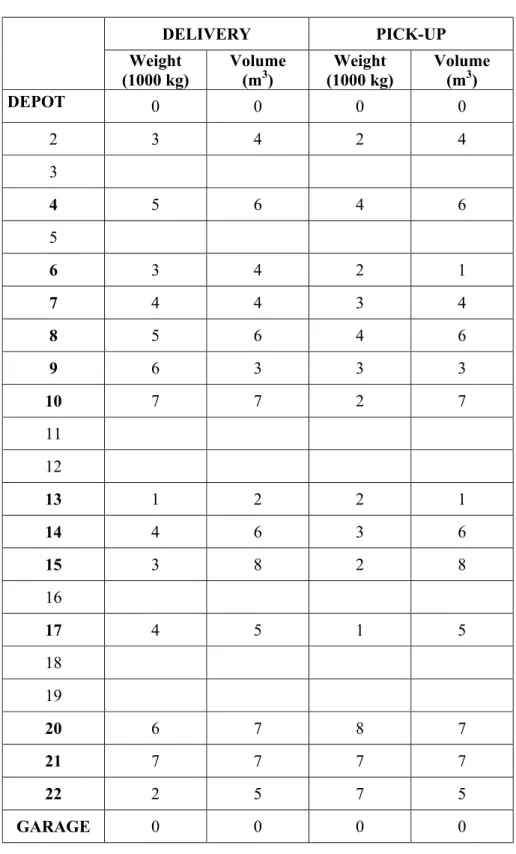
Nodes When Six Vehicles are Employed in the Model. 41 Table 3.5. Total Distances, Costs and Savings for Weeks in Case1. 42 Table 3.6. Total Distances, Costs and Savings for Weeks in Case 2. 43 Table 3.7. Total Distances, Costs and Savings for Weeks in Case 3. 45 Table A.1. Demand (pickup/delivery) Quantities of Points for Week 1. 57 Table A.2. Demand (pickup/delivery) Quantities of Points for Week 2. 58 Table A.3. Demand (pickup/delivery) Quantities of Points for Week 3. 59 Table A.4. Demand (pickup/delivery) Quantities of Points for Week 4. 60 Table A.5. Demand (pickup/delivery) Quantities of Points for Week 5. 61 Table A.6. Demand (pickup/delivery) Quantities of Points for Week 6. 62 Table A.7. Demand (pickup/delivery) Quantities of Points for Week 7. 63 Table A.8. Demand (pickup/delivery) Quantities of Points for Week 8. 64
ENGLISH-TURKISH MEANINGS OF SOME MILITARY
TERMS
Turkish Land Forces: Türk Kara Kuvvetleri Corps: Kolordu
Division: Tümen
Brigade: Tugay
Branch: Askeri sınıf (Ordudonatım, muhabere, vb.)
Ordnance Corps: Ordudonatım sınıfı
Signal Corps: Muhabere sınıfı
Engineers Corps: İstihkam sınıfı
Quartermaster Corps: Levazım sınıfı
CHAPTER 1
INTRODUCTION
Turkish Land Forces have implemented many modifications in its structure to catch up with technological development in recent years. In the context of these modifications, Turkish Land Forces have started projects about logistics that plays an important role for the Land Forces to perform its duty written in the Constitution. Establishing a unit managing all logistic efforts was one of these projects started. For that purpose, Logistics Command was established in 1988.
Logistics, which stems from the word “logisticus” belonging to Medieval Latin, means “the planning and control of the flow of goods and materials through an organization”[19]. A logistic system can only be achieved on the basis of a functional, economical and effective transportation system. Transportation is a technical service, which arranges the movements and replacements of the units, personnel and items regarding to requirements of the management and control of the operations and logistics. For this purpose, Transportation Command was formed with the order of Logistics Command, which is in charge of logistics on behalf of Turkish Land Forces. It is the mission of Transportation Command to meet the transportation demands of the units of the Land Forces in time with economical and secure means.
Transportation Command uses three modes of transportation to perform its task. These are Airway Transportation, Railway Transportation and Ring (Highway) Transportation. A modern transportation concept is based on the principle of delivering goods from an address to demanding address or picking up goods from demanding address to another address. Recently, Railway Transportation and Ring Transportation have been in preference among the transportation systems in Land Forces since they are more economical and secure.
Ring Transportation system is composed of Central Ring Transportation System (CRTS) and Regional Ring Transportation System (RRTS). CRTS satisfies transportation demands through Logistics Command’s depots, military factories and armies whereas RRTS meets transportation demands inside of Armies’ and Corps’ own responsibility areas. In order to run CRTS, a Mid-Level Auto Transportation Battalion Command was formed in Yenikent, Ankara in 2001. On the other hand, RRTS is run locally by its own Light-Level Auto Transportation units of Army/Corps/Division/Brigade.
1.1 CENTRAL RING TRANSPORTATION SYSTEM (CRTS)
CRTS’s mission is to deliver items from Main Depot to points (units, depots, factories) and to pick up items from points to bring to Main Depot. Delivering to points is called as Provision. The existing types of provision are explained in Section 1.1.1. Picking up depends on the demand points requiring those items in their own areas be sent to Main Repair Factories in Ankara through Main Depot, i.e., to send a defective machine, weapon and ammunition for repair.
As mentioned above, CRTS is performed by Mid-Level Auto Transportation Battalion Command in Yenikent, where Main Depot of Logistics Command is also situated. Related to The Joint Support Concept of Land Forces; ordnance, signal, engineer and quartermaster corps are combined under one unit to provide cooperative purchase, sharing depot resources and combining transportation efforts. So, Main Depot was formed in Yenikent in addition to depots in Army/Corps regions.
1.1.1 Provision Types of Land Forces
There are mainly two types of provision in military.
demand
Units Depot
items
Push System: Provision is provided periodically. Logistics Command makes plans to send items to the units periodically. There is no need for the units to make requests for items.
Units items Depot
In order to prevent system faults in both systems and to control the provision, Material Management System cooperating with Depot Managements in Logistics Command was established to manage all branches of items in Main Depot and other depots.
1.1.2 The Current and The proposed CRTS
In the current CRTS, five fixed routes are performed every week. The points representing the units, depots and factories on routes were selected by Transportation Command regarding size , importance, function and previous demands. All demands (pick-up/delivery) must be satisfied in three days following the vehicles’ departure.
CRTS delivers to the points in two occasions. First, points can request any item from Main Depot at any time and inform Mid-Level Auto Transportation Battalion Command and Main Depot Management (Pull System). Then, CRTS delivers to these points. Secondly, Points are delivered periodically. Main Depot knows when to deliver to the points without being informed (Push System). The word “delivery demand” will stand for two occasions in the following parts of our study. The points having delivery demand can be named as Linehaul points.
CRTS also picks up items from the points. The points make “pick-up demand” when they have any item to send to Main Depot or to the factories in Ankara.
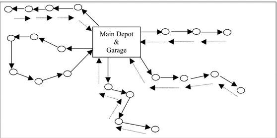
In the current system, points have a tendency not to inform Mid-Level Auto Transportation Battalion Command and Main Depot Management about their pick-up demands since points are sure to be visited. This effects vehicle utilization and creates problems in transportation. Figure 1.1 shows the current CRTS. The points having pick-up demand can be named as Backhaul points.
Figure 1.1 Routes of the Current System
Each vehicle is assigned to a tour and then loaded in Main Depot after Mid-Level Auto Transportation Battalion Command and Main Depot Management have gotten information of delivery demand quantities of the linehaul points on vehicles’ routes. The vehicle fleet loaded with delivery demands come back to Garage with the load that they picked up from the backhaul points after completing the routes.
As seen in Fig.1.1, one of the routes is a cycle and others are two-way trips on a route. Fifteen points included on the two-way routes are visited twice a week while six points included by the cyclic route are visited once. This application brings fixed travel distance and fixed cost for each week since five fixed routes are performed even if some points on the routes have zero demand. It is clear that this fixed travel distance (cost) includes unnecessary distance (cost) because of re-visiting some points and ignoring non-demanding points.
Main Depot & Garage
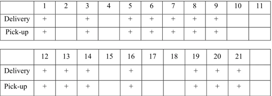
Our aim is to develope a mathematical programming model to provide a better operational system for CRTS. In our mathematical model, only demand points are visited and these points are visited only once a route. To give an example, let us assume that fourteen points have demands (pick- up/delivery) and these points inform Mid-Level Auto Transportation Battalion Command and Main Depot Management about their demand quantities. The other characteristics of the problem (volume&weight quantities, time windows, vehicle capacities, speed, load/unload times) are explained in details in Chapter 3.We only aim to show the improvement in travel distance (cost) in this part. Table 1.1 shows these demanding (pick-up/delivery) points.
1 2 3 4 5 6 7 8 9 10 11 Delivery + + + + + + + Pick-up + + + + + + + 12 13 14 15 16 17 18 19 20 21 Delivery + + + + + + + Pick-up + + + + + + +
Table 1.1 Demanding Points of the Sample Problem
Optimal solution of our Mixed-Integer Programming Model is shown in Figure 1.2.The points in black are demanding points. To comply with the current system, we employed five vehicles.
Figure 1.2 Routes of Sample Problem Solved by The proposed Model. Main Depot
& Garage
Vehicle fleet visits only demanding customers and just once. This application enables us to get rid of unnecessary distance (cost). It can easily be seen that less than five vehicles are sufficient to meet the demand in the sample problem. So, instead of employing fleets of five vehicles every week, we can also determine the vehicle fleet size giving the optimal solution by considering the number of demanding points.
In this thesis, our goal is to investigate how the total distance (cost) is affected when the proposed system for CRTS is employed. We have developed a mixed-integer programming model for solving this problem. The model determines which routes will be followed, and assigns demands (pick-up/delivery) to vehicles. Its objective is to minimize distance and transportation costs. The model is solved for eight-week data for three cases. To compare the proposed system with the current system, the model is solved for a fleet of five vehicles in Case 1. In Case 2 and Case 3, the model is solved for fleets of four and six vehicles fleet, respectively. To determine the most suitable vehicle size to satisfy the demands of points belonging to these eight-week data, cases are compared according to the total distance and cost.
CHAPTER 2
LITERATURE REVIEW
In this chapter, we give a brief review of the literature on problem related to vehicle routing problem, starting with the traveling salesman problem (TSP) and its variations.
2.1 The TSP and m-TSP
The Traveling Salesman Problem (TSP) is one of the most widely studied combinatorial optimization problems. TSP has interested many mathematicians and computer scientists specifically, because it is so easy to describe and so difficult to solve. Its statement is deceptively simple and yet it remains one of the most challenging problems in Operational Research. Hundreds of articles have been written on TSP. The reader is directed to Lawler et al [41] and Burkard [9], for a comprehensive survey of major research studies up to now.
The first use of the term “traveling salesman problem” in mathematical circles goes back to 1832. In that year, a book was printed in Germany entitled “Der Handlungsreisende, wie er sein soll und was er zu Thun hat, um Auftrage zu erhalten und eines glücklichen Erfolgs in seinen Geschäften gewiss zu sein. Von einem alten Kommis-Voyageur“ (‘The Traveling Salesman , how he should be and what he should do to get Commissions and to be Successful in his Business. By a veteran Traveling Salesman’). Although devoted for the most part to other issues, the book reaches the essence of the TSP in its last chapter: ‘By a proper choice and scheduling of the tour, one can often gain so much time that we have to make some suggestion… The most important aspect is to cover as many locations as possible without visiting a location twice…’(Voigt, 59). We don’t know who brought the name TSP into mathematical circles, but there is no question that Merrill Flood [23] is most responsible for publicizing it within that community and the operations research fraternity as well. In 1948, Flood
popularized the TSP at the RAND Corporation, at least partly motivated by the purpose of creating intellectual challenges for models outside the theory of games. A prize was offered for a significant theorem bearing on TSP.
Another reason for the popularity of the problem was its intimate connection with prominent topics in combinatorial problems arising in the new subject of linear programming. As mentioned before, the TSP was like those other problems, but apparently harder to solve, and the challenge became an intriguing issue.
In its most basic form, TSP is the problem of finding the shortest route in a given graph which starts and ends at the same node, called the origin, with all the other nodes visited exactly once.
A generalized version of the well-known TSP is the Multiple Traveling Salesman Problem (m-TSP). Furthermore, the characteristics of the m-TSP seem more appropriate for real life applications where there is a need for more than one salesman.
2.1.1 Mathematical Formulation of the m-TSP
The m-TSP is the problem of finding a set of routes for m salesmen, such that the total distance traveled or the cost is minimized. Consequently, in a feasible solution, there will be m distinct tours all containing the origin such that all the nodes are covered.
Let G = (V, A) be a graph where V 1, 2,...,=
{
n}
is the set of nodes (vertices) and A i j{
{ , }: , , i j ∈ V i≠ j}
is the set of edges, and let C = (c ) be a ij distance (cost) matrix associated with A. The m-TSP, then, is the problem of finding the minimum cost circuits in G. (Circuit is a graph cycle (i.e., closed loop) through a graph that visits each node exactly once.) The distance (cost) matrix mentioned above can be of different types. It will be useful to distinguish between the cases where C is symmetric, i.e. when cij =cji for all , Vi j∈ , andthe case where it is asymmetric, i.e. when cij ≠cji for some , Vi j∈ . C is said to satisfy the triangle inequality if and only if cij+cjk ≥cik for all , , i j k ∈ V. This occurs in Euclidean Problems, i.e. when V is a set of points in R2 and c is the ij straight-line distance between j and i.
The m-TSP is generally formulated as an integer linear program (ILP) based on the assignment model as follows. Let,
1,if arc ( , ) is in the tour 0, otherwise ij i j x = ij
x is a 0-1 variable indicating whether or not a salesman goes directly from node i to city j.Then we would like to find x which are to become 1, i.e. finding the ij edges that salesman should go through, for the distance traveled or cost to be minimized.
Miller, Tucker and Zemlin’s Formulation
The first Integer Linear Programming formulation (ILP) for the m-TSP was given by Miller, Tucker and Zemlin (MTZ) [47]. In the formulation of MTZ, the salesman turns back to the origin, denoted by 0, t times.
Minimize
0 0, n n ij ij i j i j c x = = ≠
∑ ∑
Subject to 0 1 n i i x t = =∑
(2.1) n i=0 1, 1, 2,..., ij x = j= n i≠ j∑
(2.2) 0 1, 1, 2,..., n ij j x i n j i = = = ≠∑
(2.3)ui−uj+ pxij≤ −p 1 1≤ ≠ ≤i j n (2.4)
ui∈R ∀ =i 1,...,n
xij∈
{ }
0,1 ,∀i jTheconstraint (2.1) forces the salesman to turn back to the origin exactly t times. The constraints (2.2) and (2.3) are the usual degree constraints of an assignment problem. They proposed constraint (2.4) by using extra variable in order to reduce the number of exponentially growing subtours, which do not include the origin. These constraints are generally called subtour elimination constraints (SEC). In constraint (2.4), p is the maximum number of nodes that a salesman is allowed to visit and ui are arbitrary real numbers.
2.1.2 Solution Methods of m-TSP
The TSP and m-TSP problems belong to the class of combinatorial optimization problems, known as NP-complete. Specifically; if one can find an efficient algorithm (i.e., an algorithm that will be guaranteed to find the optimal solution in a polynomial number of steps) for the TSP and m-TSP problems, then efficient algorithms could be found for all other problems in the NP-complete class. To date, however, no one has found a polynomial-time algorithm for the m-TSP. Exact methods to find an optimum solution require too much computation time, whereas heuristic approaches need much more less computational effort, but do not guarantee optimality.
The solution methods found in the literature for the m-TSP can be discussed in three categories. These are exact solution methods including branch-and-bound approach, branch-and-cut approach and cutting plane algorithm, heuristics including extended TSP heuristics and neural networks, and transformations. Although m-TSP is an important extension of TSP there is not much work done on the problem. For a detailed review of these solution methods, the reader is directed to Bodin et al [6],Laporte [37] and Lawler et al [41].
2.1.2.1 Exact Solution Methods for m-TSP
A number of exact solution methods proposed for the m-TSP are based on Integer Linear Programs (ILPs) formulations and algorithms. The most promising exact methods seem to be bound approach, branch-and-cut approach and branch-and-cutting plane algorithms.
The branch-and-bound algorithm can formally be stated as relaxing some of the constraints initially and at each iteration either finding a different lower bound for the value of the optimal solution for the current subproblem or “fathoming” the current subproblem by showing that it does not contain a feasible solution. If the subproblem cannot be fathomed, it is further split into other subproblems containing the feasible solution of original problem. Svestka and Huckfelt [56] employed their formulation in a branch-and-bound framework developed by Bellmore and Malone [6] with a new set of SECs. Gavish and Srikanth [26] employed branch-and-bound algorithm to solve m-TSP by relaxing one of the constraints given below :
Degree Constraints: ( They require each node to be visited only once ) SEC: (They eliminate tours not including the origin )
Integrality Constraints: ( They force all variables in the optimal solution to be integer )
The algorithm basically starts with solving the associated assignment problem (AP). However the solution of the corresponding AP requires the augmentation of the original distance matrix. If there exists any subtours in the solution, a subset of subtour elimination constraints are introduced and the resulting AP is solved as an integer programming again. The procedure repeats itself until there are no subtours and the solution satisfies all the constraints of the ILP formulation.
The cutting plane technique is based on relaxing the original problem and continuously tightening the lower bound by introducing extra cuts, thus getting a
relaxation value close to the optimal integer value. The most commonly used inequalities for cuts are SECs, comb inequality, clique tree inequality, path, crowns and ladder inequality. For detailed information the reader is directed to Jünger et al [32]. The first example of cutting plane method was due to Dantzig, Fulkerson and Johnson [15]. They proposed a method for solving TSP and showed the power of this method by solving 49-city TSP. Laporte and Nobert [39] introduce a cutting plane algorithm for the m-TSP similar that of Svestka and Huckfeld, without modifying the original distance matrix. The algorithm can be extended to have the number of salesman fixed or variable, or the objective function to include a fixed traveling cost.
Branch-and-cut approach uses the cutting planes in a branch-and-bound scheme to obtain better relaxations. It means that for each partition of the solution set of LP relaxation, several cuts are added to the current formulation to tighten the problem. That is in bounding step, instead of solving one relaxation; a sequence of relaxation is solved each time adding an inequality that is violated by the current fractional solution. Various branch-and-cut techniques have been proposed for solving m-TSP. Some of these can be found in the papers of Hong in 1972, Miliotis in 1976, Padberg and Hong in 1980. Applegate et al [2] uses a new branch and cut type method to obtain a solution of 13,509-city instance.
2.1.2.2 Heuristic Solution Methods for m-TSP
In order to obtain a “near-optimal” solution in a reasonable amount of time instead of finding the optimal solution in more expensive way, many heuristic solution techniques have been introduced for the TSP and m-TSP. Many heuristics developed for TSP are applied to m-TSP by transforming it to standard TSP. Heuristic solutions can be grouped in two. The First is Tour Construction Heuristics and the second is Tour Improvement Heuristics.
These types of heuristics build an approximately optimal tour starting from the original distance matrix according to a construction procedure. The procedure stops without trying to improve it, once it has found a feasible solution. In the tour construction procedures the following three components serve as key ingredients: The choice of an initial tour, the selection criterion, the insertion criterion.
Christofides [10] developed a construction heuristic on the base of spanning trees and minimum weight matching. Johnson and McGeoch [31] proved that this procedure has a computation time of O(n3). But later on, Reinelt [51] showed that computation time can be reduced to O(n2).
In Nearest Neighbor Heuristics, the simplest of all the heuristics, the procedure starts from an initial node arbitrarily and each step moves to the next nearest node, which was not visited yet. After all the nodes are visited, the tour is finally accomplished by linking the last visited node to the initial starting node. By considering all the n vertices as the starting point, the computation time of this procedure can grow up to O (n3) from O (n2) (Laporte, 37).
Insertion Algorithm starts with a small subset of nodes and enlarge this subset by inserting the nodes, which are not included in the subset. While inserting, the procedure uses insertion criterions. The computation time of this procedure can grow up to O(n3) from O(n.logn) depending on the insertion criterion (Laporte, 37).
Another tour construction heuristic is The Savings Algorithm having derived from the vehicle routing algorithm proposed by Clarke and Wright [13]. This heuristic will be explained in detail in Section 2.2.2. The computation time of this procedure is O (n2.logn), but the storage space for savings require a space of O (n2) Reinelt [51].
Tour Improvement Heuristics try to improve a feasible tour by simple tour modifications after an initial tour is obtained by the use of tour construction heuristics. Tour improvement heuristics are performed according to a specified order of operations until a tour for which no operation yields a better tour is reached. These specified order of operations could be assumed as a local search method because better tours obtained are only local optimum tours.
Lin [44] proposed the r-opt algorithm where r edges in a feasible tour are exchanged for r edges not in that optimal solution as long as the result remains a tour and the length of that tour is less than the length of the previous tour. An improvement to Lin’s r-opt algorithm is due to Lin and Kerninghan [45], where the value of r changes dynamically during the algorithm.
Simulated Annealing Heuristics remove the disadvantage of r-opt algorithm, which can get stuck at local optima by moving from a given initial solution to a minimum –cost solution by changing the initial solution gradually. However, sometimes, the initial solution is substituted by the new solution although the new solution is more costly. This increases the probability of getting closer to the global optimum. Many authors have proposed the application of simulated annealing to the TSP. Some of these are due to Rossier et al. [53] and Nahar et al. [49].
Tabu search heuristics are similar to the simulated annealing in the way of prevention from getting stuck at local optima. These kinds of heuristics have become popular for the last decades. The solutions which have already been examined are stored in ‘tabu list’ to prevent cycling. The tabu search has been applied to the TSP with numerous successful results. Some of these are due to Knox [34], Malek [46] and Fiechter [20].
Genetic algorithms (GA) have been recent approach to the combinatorial optimization type problems. GAs are actually based on human genetics, trying to imitate the natural evolution scheme and known to find near-optimal solutions to highly complex problems. For the case of TSP, the chromosomes are used to
represent the tours are generally coded as the order of visited vertices or edges in the graph. Detailed discussions on the subject can be found in Grefenstette al [29].
2.1.2.3.Transformations to the TSP
Third group for the solution methods of m-TSP is the transformation of the problem to a single TSP. By transformation, m-TSP can be solved by any algorithm developed for TSP. Orloff [50], work of whose demonstrates that solving any m-TSP is equivalent to a TSP solution on a transformed graph.He transformed m vehicle General Routing Problem (m-GRP) into a single vehicle GRP on the same graph.
Bellmore and Hong [4] showed that the asymmetric case of the m-TSP with m salesman and n nodes could be converted into a standard asymmetric TSP containing (n+m-1) nodes. Hong and Padberg [30] proposed a similar work to that of Bellmore and Hong where symmetric m-TSP with m salesman and n nodes is transformed into a standard symmetric TSP containing (n+m-4) , considering the fixed charges as well.
2.2. VEHICLE ROUTING PROBLEMS (VRP)
Vehicle Routing, which is called “one of the great success stories of operations research in the last decade”, is distinguished by a highly successful interplay between algorithmic techniques and the development of effective routing systems for industry. On the one hand, operations researchers with academic affiliations have gone beyond the design and development of algorithms to play an important role in the implementation of routing systems. On the other hand, developments in computer hardware and software and their growing integration into operational activities of commercial concerns have created a high degree of awareness of potential benefits of vehicle routing. The interested reader may consult a number of useful surveys of the field including Golden and Assad [28], Bodin et al [6], Bott and Ballaou [7],Christofides [11].
The Vehicle Routing Problem (VRP) is a distribution problem in which a set of customers with known locations and requirements for some commodity is to be supplied from a single depot using a set of delivery vehicles each with a prescribed capacity. From a graph theoretical point of view the VRP may be stated as follows: Let G (V, A) be a complete graph with node set V =
{
0,1,...,n}
and arc set A i j{
( , ) : , , i j ∈ V i≠ j}
. In this graph model, node “0” is the depot and the other nodes are the customers to be served. Each node except from the depot is associated with known demands di. For every arc, there is anassociated cost cij,(i≠ j), representing the travel cost (distance, time) between
nodes i and j. There are m identical vehicles based at the depot, having same capacity Q. The VRP consists of designing a set of least-cost vehicles in such a way that each node excep the depot is visited exactly once by exactly one vehicle to satisfy its demand; all vehicle routes start and end at the depot, vehicle capacities are not exceeded and some other side constraints are satisfied.
The VRP can have different aspects that form the characteristics of the problem. Some of these are: Nature of demand (pure pick-ups or pure deliveries, pick-ups or deliveries with backhaul option, single or multiple commodities, priorities for customers), information on demand (known in advance, changeable by time), vehicle fleet (fixed or variable fleet size, one or more than one) homogeneous fleet or multiple vehicle types), depot (single or multiple), scheduling requirements (time windows for pick-up/delivery (soft, hard), load/unload times).
2.2.1 Mathematical Formulations of VRP
Most of the VRP problems with underlying characteristics listed above are well defined mathematically, and they are extremely difficult in NP-hard class. This difficulty in the problem induced researchers to develop heuristic solution procedures in addition to optimization algorithms. We present general models where a set of customers is served by m non-identical vehicles based at a depot with a set of routes whose total distance (travel cost) is minimized for
Capacitated Vehicle Routing Problem (CVRP), Vehicle Routing Problem with Backhaul (VRPB) and Vehicle Routing Problem with time windows (VRPTW).
Dantzig and Ramser Formulation
Dantzig and Ramser (DR) [14], who proposed a formulation for single depot VRP with vehicle with capacity and maximum cost (time or distance) constraints, considered the VRP for the first time in the literature. The formulation is given as follows:
Minimize 1 1 1 N N N ij ijk i j k c x = = =
∑∑∑
Subject to 1 1 1, 1,2,..., 1 N N ijk i k x j N = = = = −∑∑
(2.20) 1 1 1, 1, 2,..., 1 N N ijk j k x i N = = = = −∑∑
(2.21) 1 1 0, 1, 2,..., , 1, 2,..., N N ihk hjk i j x x k V h N = = − = = =∑
∑
(2.22) 1 1 1, 2,..., N N i ijk k i j Q x P k V = = ≤ =∑ ∑
(2.23) 1 1 1, 2,..., N N ij ijk k i j c x T k V = = ≤ =∑∑
(2.24) 1 1 1 1, 2,..., N Njk j x k V − = ≤ =∑
(2.25) 1 1 1 1, 2,..., N iNk j x k V − = ≤ =∑
(2.26) xijk∈{ }
0,1 , ,∀i j k1 1 1 1 i j ijk y y Nx N i j N k V − + ≤ − ≤ ≠ ≤ − ≤ ≤ (2.27)
In the formulation, V vehicles, say {1,…,V ) based at a depot (node N) with capacities Pk respectively visit the customers whose demands are Qi .Tk stands
for maximum cost allowed for a route of vehicle k. xijh is 0-1 variable and xijk=1
if pair i,j is in the route of vehicle k , 0 otherwise. Constraints (2.20) and (2.21) are usual assignment constraints. Route continuity is represented by constraint (2.22). Constraint (2.23) represents the vehicle capacity constraints. Constraint (2.24) represent the total route constraint. Constraints (2.25) and (2.26) make certain that vehicle availability is not exceeded. Finally constraint (2.27) is SEC. In this model, it has been assumed that whenever a customer is serviced, his requirements are satisfied.
Desrochers, Savelsberg, Lenstra and Soumis Formulation
Minimize ( , )i j A ij ij c x ∈
∑
Subject to ij 1, for j N x i N ∈ = ∈∑
(2.28) ij ji 0, for j N j N x x i N ∈ ∈ − = ∈∑ ∑
(2.29) Di+ ≤tij Dj for ( , )i j ∈I (2.30) ei≤Di≤li for i N∈ (2.31) yi+qij≤ yj for ( , )i j ∈I (2.32) 0≤ yi≤Q for i N∈ (2.33) xij∈{ }
0,1 ∀,i jIn the formulation of Desrochers, Savelsberg, Lenstra and Soumis [16] for VRPTW, xij is a 0-1 variable and xij =1 if a vehicle visits customer j immediately
after customer i, and 0 otherwise. Q stands for the capacity of the vehicle, cij
represents the travel cost between customers i and j .tij is the travel time between
customer i and j. For each customer, there is a demand qi and time window [ei,li] which identifies the earliest and latest time to be visited , respectively. We note that the number of vehicles is not bounded in the formulation.
Constraints (2.28) and (2.29) are usual assignment constraints. Constraints (2.30) and (2.31) guarantee feasibility of the schedule and constraints (2.32) and (2.33) ensure feasibility of the loads.
Toth and Vigo Formulation
Toth and Vigo [58] proposed an integer linear programming model for VRPB in asymmetric distance matrix. They grouped the vertices as Linehaul (L) and Backhaul (B). Let Λ (respectively Β) be the family of all subsets of vertices in L (respectively B), and let Φ=Λ ∪ Β. For each S∈Φ, let σ (S) be the minimum number of vehicles needed to serve all the costumers in S. For each i,
{
}
{
}
+
-i i
Γ = j i j: ( , )∈A and Γ = j: ( , )j i ∈A where A is the arc set. In the formulation K is the number of vehicles and depot is node 0.
Minimize ( , ) ij ij i j A c x ∈
∑ ∑
Subject to 1 j ij i x j V − ∈Γ = ∈∑
(2.34) 1 i ij i x i V + ∈Γ = ∈∑
(2.35) 0 0 i i x K − ∈Γ =∑
(2.36)0 0j j x K + ∈Γ =
∑
(2.37) \ ( ) j ij j S i S x σ S − ∈ ∈Γ ≥∑ ∑
(2.38) \ ( ) i ij j S i S x σ S + ∈ ∈Γ ≥∑ ∑
(2.39) xij ∈{ }
0,1 ,∀i jConstraints (2.34), (2.36) and (2.35),(2.37) impose indegree and outdegree constraints for the customer and the depot vertices, respectively. Constraints (2.38) and (2.39) impose both connectivity and the capacity constraints.
Kulkarni and Bhave Formulation
A simple formulation based on that of DR was proposed by Kulkarni and Bhave [36]. In the formulation L is the maximum number of nodes which a vehicle can visit and Qi is the demand of node i. If P is the capacity of all the vehicles and T
is the maximum cost allowed for a route for the vehicle, then for a single depot VRP formulation is as follows: Minimize 1 1 N N ij ij i j c x = =
∑∑
Subject to 1 1, 1, 2,..., 1 N ij i x j N = = = −∑
(2.40) 1 1, 1, 2,..., 1 N ijk j x i N = = = −∑
(2.41) 1 , N Nj j x V = ≤∑
(2.42) 1 , N iN i x V = ≤∑
(2.43)xij∈
{ }
0,1 ,∀i j yi−yj+Lxij≤ −L 1 1≤ ≠ ≤ −i j N 1 (2.44)ui−uj+Pxij ≤ −P Qi 1≤ ≠ ≤ − (2.45) i j N 1
vi− +vj Txij≤ −T 1 1≤ ≠ ≤ − (2.46) i j N 1
In the above formulation, constraints (2.40)-(2.43) ensure that each node is being served only once and that all the V vehicles are being used. Constraints (2.44)-(2.46) are the subtour breaking constraints, which also represent the node constraints, capacity constraints and cost constraints respectively. In words these equations ensure that all the tours are starting and ending at the Depot N and further every route serves at the most L nodes and the load and the cost on every route are less than or equal to the vehicle capacity P and the maximum allowable cost T respectively.
But, later Achuthan and Caccetta [1] proved that formulation above fails since constraints (2.46) do not ensure that the maximum allowable cost for a vehicle tour is at most T. They redefined constraints (2.46) as:
( )
i j ij ij
v v− + +c T x T≤ (2.47) In 1988, Brodie and Waters [8] redefined constraints (2.39) in Kulkarni and Bhave Formulation as:
i j ij ij
v − +v T x ≤ −T c (2.48)
2.2.2 Solutions Methods of VRP
Almost all problems of vehicle routing are NP-hard. (Lenstra&Rinnoy Kan 43). Computational complexity theory has provided strong evidence that any
optimization algorithm for their solution is likely to perform very poorly on some occasions which means that its worst case running time is likely to grow exponentially with problem size. The solution methods of VRP may be classified as exact algorithms and heuristic algorithms.
2.2.2.1 Exact Algorithms for VRP
The usual solution methods in integer programming and combinatorial optimization are applied in the design of exact solution algorithms to the VRP. Exact methods are based on the formulations that were given before. Exact algorithms for the VRP can be classified into three broad categories: direct tree search methods, dynamic programming and integer linear programming.
Laporte,Mercure and Nobert [40] proposed an algorithm by exploiting the relationship between the VRP and one of its relaxation, the m-TSP. Given an upper bound mu on m, the m-TSP can be transformed into a 1-TSP.(Lenstra and
Rinnooy Kan 42). Then, the problem is solved through a branch-and-bound process in which subproblems are assignment problems. Using this methodology, Laporte, Mercure and Nobert [40] have solved to optimality randomly generated asymmetrical CVRP involving up to 260 vertices by partitioning the current infeasible subproblem.
Christofides, Mingozzi and Toth [12] have developed an algorithm for symmetrical VRPs. It is based on the k-degree center tree relaxation of the m-TSP where m is fixed. In any feasible solution the set E of edges are partitioned into four subsets which are (i) edges not belonging to the solution, (ii) edges forming k-degree tree center, (iii) y edges incident of vertex 1,which is depot, (iiii) m-y edges not incident to vertex 1. The core of the algorithm is to embed the lower bound on the solution in a branch-and-bound scheme. They have successfully solved VRPs ranging in size from 10 to 25 vertices.
Kolen, Rinnooy Kan and Trienekens [35] extended the state space relaxation presented by Christofides, Mingozzi and Toth. This state space relaxation is
based in a mapping from the original state space to a space of smaller cardinality. Kolen, Rinnooy Kan and Trienekens used a two-level state space relaxation for VRPTW. At the first level, a lower bound on the costs of a time-constrained path from the depot to vertex j with load q is computed. The states are of the form (t,q,j), where q is the load of a shortest path arriving at vertex j no later than time t. at the second level , a lower bound on the costs of m routes with total load
i i N
q
∈
∑
and different destination vertices is computed. The states are of the form (k,q,j), where q is the total load of the first k routes and j is the destination vertex of route k. Problems with up to fifteen customers are solved.Fisher [21] proposed an algorithm using minimum k-trees. Given a graph with n+1 nodes a K-tree is defined to be a set of n+K edges that span the graph. He showed that the vehicle routing problem could be modeled as the problem of finding a minimum cost K-tree with K edges incident on the depot and subject to some side constraints that impose vehicle capacity and the requirement that each customer be visited exactly once. The side constraints are dualized to obtain a Lagrangian problem that provides lower bounds in a branch-and-bound algorithm. This algorithm has produced proven optimal solutions for a number of difficult problems, including a well-known problem with 100 customers and several real problems with 25-71 customers.
Eilon, Watson-Gandy and Christofides [18] were the pioneers to propose dynamic programming for VRP with a fixed number of m vehicles. Let c (S) denote the cost (length) of a vehicle route through vertex1 –the depot-and all vertices of a subset S ofV \ 1{ }. Let fk(U) be the minimum cost achievable using
k vehicles and delivering to subset U of V \ 1{ }. Then the minimum cost can be determined through the following recursion:
fk(U) = { } * * * 1 \ 1 ( ) ( 1) min k ( \ ) ( ) ( 1) U U V c U k f − U U c U k ⊂ ⊆ = + > (2.49)
The solution cost is equal to fm (V \ 1{ }) and the optimal solution corresponds to the optimizing subsets U* in (2.49)
Balinski and Quandt [3] were among the first to propose a set partitioning formulation for VRPs. Consider J, the set of all feasible routes j and aij be a
binary coefficient equal to 1 if and only if vertex i > 1 appears on route j. Let cj*
be the optimal cost of route j and xj , binary variable equal to 1 if and only if
route j is used in the optimal solution. The problem can then be formulated as follows: Minimize * j j j J c x ∈
∑
Subject to ij j 1 ( \ 1 ){ } j J a x i V ∈ = ∈∑
(2.50) xj∈{ }
0,1 (j J∈ )There is at least one exact procedure for VRPB developed by Yano et al [60]. This procedure uses set covering to find an optimal set of routes. Each route can at most have four points. All such routes are generated ant the optimal route sequencing is found by complete enumeration.
Mingozzi, Giorgi and Baldacci [48] described a procedure for VRPB that computes a valid lower bound to the optimal solution cost by combining different heuristic methods for solving the dual of the LP-relaxation of the exact formulation.
In the Toth and Vigo’s [60] new integer linear programming model mentioned in Chapter 2.2.1, a Lagrangian lower bound, which is strengthened in a cutting plane fashion for VRPB in symmetric and asymmetric versions is proposed. The model is used to derive a Langrangian lower bound, based on projection of the
shortest spanning arborescence with fixed degree at the depot vertex and the optimal solution of min-cost flow problems.
Desrosiers, Soumis and Desrochers [17] apply branching on flow variables when time windows are very tight for VRPTW. They solved problems up o 150 customers. Sörensen [54] suggests the use of Lagrangean decomposition for VRPTW. The two resulting sub problems are the shortest path problem with time window and the generalized assignment problem. But no computational results were reported.
2.2.2.2.Heuristic Algorithms for VRP
Heuristic algorithms for the VRP can often be derived from procedures derived from the TSP.(Laporte,38). Several families of heuristics proposed for the VRP can be classified into two main classes: classical heuristics developed mostly between 1960 and 1990, and metaheuristics whose growth has occurred in the last decade. Most standard construction and improvement procedures in use today belong to the first class. These classical heuristics performs in limited exploration of search space. Nevertheless, they can produce good solutions. In metaheuristics, a deep exploration of search space is performed. Combining neighborhood search rules, memory structures, are effective in metaheuristics. They can produce higher quality solutions than classical heuristic can. But, it is clear that the price to pay is increased computing time.
Clarke and Wright’s saving algorithm [13] was first proposed in 1964 to solve CVRP which has unlimited number of vehicles. The method is based on to merge two routes according to the largest savings that can be generated. The savings sij =ci1+c1j− for ,cij i j=2,...,n and n-1 vehicle routes are created. The savings are ordered in a non-increasing way. Then, routes are merged as in the following example. Let two vehicle routes contain (i,1) and (1,j) ,respectively. If sij > 0 these two routes are merged by introducing arc (i,j) and
feasible. The procedure is repeated until no improvement is possible. This procedure has O(n2log n ) operation time.
One of the classical approaches of the VRP is Fisher and Jaikumar [22] algorithm, which is also named in cluster-first, route-second algorithms. These kinds of algorithms solve a Generalized Assignment Problem (GAP) in order to form the clusters instead of using a geometric method. The Fisher and Jaikumar algorithm includes the following step.
• Choose seed points j in V to initialize each cluster k. (seed selection) k
• Compute the cost d of allocating each customer i to each cluster k ik as min
{
0 0 (,
0 0}
0 0).k k k k k k k
ij i ij j j j i i j j
d
=
c
+
c
+
c
c
+
c
+c
−c
+
c
(allocation)
• Solve a GAP with costs dij , customer weights qi and vehicle capacity Q.
(generalized assignment)
• Solve a TSP for each cluster corresponding to the GAP solution.(TSP solution)
In the algorithm, the number of vehicle routes m is fixed and relating to the customer weights the plane is parted into m cones. The seed points are dummy customers located along the rays bisecting the cones. After having determined the clusters, the algorithm solves the TSPs optimally using a constraint relaxation based approach.
The last group of classical heuristics is improvement heuristics. Improvement heuristics for VRP are performed on each seperate vehicle route or on several routes at a time. Most improvement procedures for TSP are based on r-opt algorithm Lin-Kernighan. As explained before, r edges in a feasible tour are exchanged for r edges not in that optimal solution as long as the result remains a tour and the length of that tour is less than the length of the previous tour.
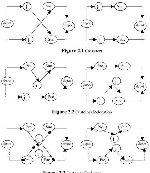
Thompson and Psaraftis [57] and Kindervater and Savelsbergh [33] propose descriptions of multi-route exchanges for the VRP.In these papers tours are not considered in isolation. Paths and customers are exchanged between different tours until no further improvements can be obtained. Figure 2.1, Figure 2.2 and Figure 2.3 show the Crossover, Customer Relocation and Customer Exchange operations, respectively.
Figure 2.1 Crossover
Figure 2.2 Customer Relocation
Figure 2.3 Customer Exchange
One group of the metaheuristics is tabu search heuristics. It starts form an initial solution x and moves at each iteration t from 1 x to its best neighbour t xt+1, until a stopping criteria ‘s satisfied. To avoid cycling, solutions that were recently examined are forbidden, or tabu. In order to reduce time and memory requirements, it is generally accepted to record an attribute of tabu solutions
depot i Suc j Suc depot depot i Suc j Suc depot depot Prei Suc j Suc depot depot Suc j Suc depot i Prei i depot Prei Suc Prej Suc depot depot Suc Suc depot j Prei i i i Prej
rather than solutions themselves. Rochat and Taillard [52] proposed Tabu search with set-partition based heuristic where an adaptive memory is kept as a pool of good solutions.
Gendreau, Hertz and Laporte [27] present a GENI procedure related to the tabu. When applied to classical VRPs described in the literature, the proposed heuristic may be one of the best ever developed for the VRP regarding the results they found.
A new metaheuristic approach inspired by foraging behavior of real colonies of ants is Ant Colony Optimization (ACO). The basic ACO idea is that a large number of simple artificial agents are able to build good solutions to hard combinatorial optimization problems via low-level based communications. Real ants cooperate in their search for food by depositing chemical traces on the floor. An artificial ant colony simulates this behavior. Artificial ants cooperate by using a common memory that corresponds to the pheromone deposited by real ants. This artificial pheromone is one of the most important components of ant colony optimization and is used for constructing new solutions. Gambardella, Taillard and Agazzi [24] used ant colony system to solve VRP. In their paper, VRP is transformed into a TSP by adding m-1 new depots A sample is picturized in Figure 2.4 Ants are used to compute complete feasible tours. Local search that exchange paths and customers is executed.
d2 d3
d1 d0
CHAPTER 3
ANALYSIS OF THE PROBLEM and
MATHEMATICAL FORMULATION
In this thesis, our objective is to develop and solve a model that determines the optimal routes, which vehicle fleet will follow and provides a method for assigning demands (pick-up/delivery) to vehicles. Best fleet size will be determined by comparing the optimal solutions for alternative sizes.
It is the aim of the Ring Services System to deliver items to points and to pick up items from points within three days if there is a demand (pick-up/delivery). The fleet is loaded regarding to points’ demands in the Main Depot, where all kind of items is stored. After having performed the routes, the fleet loaded with pick-ups comes back to the Garage, which is near the Main Depot.
This process is repeated every week. As explained in Section 1.1, five fixed routes are performed in the current system regardless of demands (pick-up/delivery). Although a point doesn’t have any demand (pick-up/delivery), one vehicle of the fleet must visit this point anyway, according to the current system. So, the fleet makes a lot of unnecessary mileage. For each week, Transportation Command has a fixed distance and cost of these five fixed routes. Provided that Transportation Command knows in advance which of the points have demands (pick-up/deliver), the fleet visits only these points and can do away with the unproductive mileage. It is clear that the fixed cost for each week will be reduced by this method.
3.1. DATA FILE
Mid-Level Auto Transportation Battalion Command, which is responsible for performing Central Ring Transportation System (CRTS) as a subordinate unit
of Transportation Command, has a very detailed documentation of past years. Since the CRTS started to be employed in 2001, Mid-Level Auto Transportation Battalion Command has filed the information for all weeks, i.e., weights and volumes they delivered and picked up, types of vehicles performing the routes. We used an eight-week data belonging to 2002.
3.1.1. Main Depot and Garage
Logistic Command wants to keep its safety stocks only in Main Depot. This depot is large enough to store Ordnance, Signals, Quartermaster and Engineers Corps items. Although ordnance, signal and engineers corps have their own depots as fourth level depots in the Corps region, provision except for fourth level is provided from Main Depot. There exists a strong communication network including Material Management Centers established to arrange each of the branches in Logistic Command, points, Mid-Level Auto Transportation Battalion Command and Main Depot management. Garage is located in Mid-Level Auto Transportation Battalion near Main Depot. A large number of trucks with different capacities are available here.
3.1.2. Points
The military units, factories and depots are situated throughout the country. Nearly, in all of the cities in the country a military unit or a factory or a depot is located. But regarding size, importance and function of those, twenty-one points were selected for demand (pick-up/ delivery) points. The demands (pick-up/ delivery) of military units, factories and depots out of these twenty-one points are provided by the Regional Ring Transportation System (RRTS). This issue is not related to our study. The shortest distance table is shown in Appendix A, page 65.
3.1.3.Vehicles
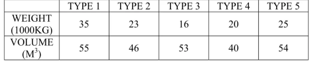
Mid-Level Auto Transportation Battalion Command has a vehicle fleet in different capacities and characteristics to perform its task. We used the same fleet of five vehicles (Case 1) as in the routes performed in eight-week data of 2002. When solving the model for fleet of four vehicles (Case 2), we excluded the Type 5 and used the first four types of vehicles, while one more Type 1 vehicle is added to fleet when fleet of six vehicles are employed (Case 3). Capacities of vehicles are shown in Table 3.1
TYPE 1 TYPE 2 TYPE 3 TYPE 4 TYPE 5 WEIGHT
(1000KG) 35 23 16 20 25
VOLUME
(M3) 55 46 53 40 54
Table 3.1. Capacities of Vehicles
Since vehicles can be refueled on their way whenever they need, it doesn’t make sense to consider how long a vehicle can travel with a full depot.
3.1.4. Items
All kind of items related to ordnance, signal, quartermaster and engineer corps are delivered and picked up with these vehicles. The volumes and weights of the items are important in the view of volume and weight capacity of vehicles. In the documentation belonging to 2002, although we know the volumes and weights of the items, we cannot get any information about contribution of specific items to these volumes and weights. Properties (volume and weight) of the items demanded (picked up/delivered) are shown in the Appendix A, pages 57-64.
3.2 ASSUMPTIONS
In order to simplify the problem and make it solvable, we make some assumptions. These are:
3.2.1. All demands (pick-up/delivery) must be satisfied
We assume that the Main Depot must meet all demands (pick-up/delivery). For delivery, it is not true in reality. Vendors and military factories supply Main Depot and Main Depot supplies the points. Main Depot may not provide every item whenever needed. As mentioned in Chapter 1, Land Forces have two types of Provision, i.e., Pull System and Push System. In real life, the situation that demands (delivery) are not satisfied may occur in Pull System, since the points may demand an item from Main Depot at any time when Main Depot does not have this item. However, because Provision is provided periodically in Push System, the probability that demands (delivery) are not satisfied in Push System is less than the Pull system. There is a schedule determining when and how much to provide units in the Push System. Items are stored in Main Depot according to this schedule and all demands (delivery) are satisfied in Push System. But in our study, we do not consider the type of Provision. It is assumed that all demands (delivery) are satisfied. Pick-up demands are independent of the type of Provision. All points can have pick-up demands whenever they have any item to send to Main Depot or factories in Ankara..
3.2.2. Demands (pick-up/delivery) are fixed and known in advance
For delivery, in Pull System, points inform Main Depot Management, Material Management Centers, Mid-Level Auto Transportation Battalion Command about their demands (delivery). In Push System, the same trio knows how much to deliver to points according to schedule. For pick-up demands, points inform Main Depot Management, Material Management Centers, Mid-Level Auto
Transportation Battalion Command about the quantities of items to be sent to Main Depot.
3.2.3.The load/unload times are fixed and known in advance.
Time to load/unload the vehicle in the points is known in advance. In real life, weather conditions, the number of personnel in loading/unloading points and disorders in loading/unloading machines may affect the length of the time.
3.2.4.Time windows are fixed and known in advance.
Each point has time intervals, i.e., earliest and latest time to be visited. Earliest time of the points are not important but all the points demanding (pick-up/ delivery) must be visited within three days following the vehicles’ departure. The fleets leave the Main Depot on Mondays and all the points on the routes must be visited by Thursday.
3.2.5. Vehicle speed is fixed and known in advance.
Each vehicle’s speed is fixed with 70 km/h during the travel. In spite of the fact that vehicles use freeways, vehicles cannot exceed the speed limit for a secure trip.
3.2.6.The number of vehicles is fixed and known in advance.
The number of vehicles is fixed. Battalion Commands has the initiative to decide on the number of vehicle fleet size at the beginning of the tours. First, we used fleets of five vehicles to compare the current system with the proposed system. We also used four and six vehicles of fleet to see if there is any improvement in total distance (cost) for different sizes of fleet.
3.3.FORMULATION
In the literature survey, we come across many ILP formulations of m-TSP and VRP. Each one has different features ( different vehicle types, pickups&deliveries, time windows, load&unload times, variable speed) and different objectives (minimize distance, minimize travel time, minimize number of vehicles, minimize total cost). We used some of the constraints in the formulations complying with our model.
3.3.1. Indices
N : Set of all the points including Main Depot and Garage. Main Depot,2,3…20,21,22, Garage.
V : Set of vehicles.
Type1, Type2…Type6.
3.3.2.Initial Data and Parameters
Cij : Distance from i to j
Tij : Travel time between i and j ( Cij/h) min
i
T : Earliest time of point i to be visited.
maxi
T : Latest time of point i to be visited. Li : Time of loading/unloading in point i.
Qv : Weight capacity of vehicle v.(1000 kg)
Bv : Volume capacity of vehicle v.(m3)
di : Quantity to be delivered to point i.(in 1000 kgs)
pi : Quantity to be picked up from point i.(in 1000 kgs)
fi : Quantity to be delivered to point i.( m3)
gi : Quantity to be picked up from point i.(m3)
h : Speed of the vehicles (70 km/h) q : The number of the vehicles