T.C.
Bahçeşehir University
POINT BASED CORRESPONDENCELESS POSE
ESTIMATION
Master Thesis
T.C.
Bahçeşehir University Institute of Science Computer Engineering
POINT BASED CORRESPONDENCELESS POSE
ESTIMATION
Master Thesis
Ferhat CANBAY
T.C
BAHÇEŞEHĐR ÜNĐVERSĐTESĐ
The Graduate School of Natural and Applied Sciences Computer Engineering
Title of the Master Thesis : Point Based Correspondenceless Pose Estimation Name/Last Name of the Student : Ferhat CANBAY
Date of Thesis Defense : 26.08.2009
The thesis has been approved by the Graduate School of Natural and Applied Sciences.
Prof. Dr. A. Bülent ÖZGÜLER Director
This is to certify that we have read this thesis and that we find it fully adequate in scope, quality and content, as a thesis for the degree of Master of Science.
Examining Committee Members:
Asst. Prof. Dr. Sezer GÖREN UĞURDAĞ (Supervisor) :
Asst. Prof. Dr. H. Fatih UĞURDAĞ :
ACKNOWLEDGEMENT
I would like to thank Dr. Sezer GÖREN UĞURDAĞ and Dr. H. Fatih UĞURDAĞ, for their guidance, encouragement, support, valuable comments and constructive suggestions throughout my study. Also I thank to my family for their understanding during the study.
ÖZET
CORRESPONDENCELESS POINT BASED POSE ESTIMATION
Ferhat CANBAY
Bilgisayar Mühendisliği
Tez Danışmanı: Yrd. Doç. Dr. Sezer GÖREN UĞURDAĞ
Ağustos 2009, 66
Günümüzde, hayatımızı kolaylaştıran teknolojilerden biri hiç kuşkusuz görüntüleme sistemleridir. Görüntüleme sistemleri yalnızca görüntüleme işi yapmayıp aynı zamanda bu görüntüyü işleyerek anlamlı veriler elde etme yeteneğine sahip sistemlerdir. Herhangi bir kamera tarafından elde edilmiş bu görüntülerde bulunan bir nesnenin pozisyon ve oryantasyon’u(poz) robotlarda, filmlerde, animasyonlar gibi bir çok alanda ihtiyaç duyulan bir bilgidir. Bu tezde poz kestirimi için gerekli olan alt görevlerden öznitelik bulma süreci otomatik hale getirilmiştir. Buna ek olarak nokta temelli, karşılıklık bilgisi gerektirmeyen Gravitational Pose Estimation (GPE) ve SoftPOSIT algoritmaları birbirlerine entegre edilmiştir. Aynı zamanda nesnenin görünmeyen noktalarından kaynaklanan problem de belli ölçülerde tolere edilmiştir. Poz kestirim kısmı, gerçek ve sanal resimler kullanılmak suretiyle test edilerek başarı oranı da ayrıca kanıtlanmıştır.
ABSTRACT
CORRESPONDENCELESS POINT BASED POSE ESTIMATION
Ferhat CANBAY
Computer Engineering
Supervisor: Asst. Prof. Dr. Sezer GÖREN UĞURDAĞ
August 2009, 66
Today, one of the technologies which ease our lives is vision systems. Vision systems not only execute the task of vision but also they have the ability to process these images to extract meaningful data. The position and orientation (pose) of an object found in these images are useful information required for many fields such as robotics, films and animations. In this thesis, we automate the subtasks such as feature extraction and blob coloring that are required during the pose estimation. In addition, a correspondenceless point-based algorithm which is called Gravitational Pose Estimation (GPE) is proposed and implemented. We have also integrated GPE and SoftPOSIT into a single method called GPEsoftPOSIT, which finds the orientation within 3 degrees and the position within 10% of the object’s diameter even under occlusion-the manner in which an object closer to the viewport masks (or occludes)an object further away from the viewport. The algorithm is evaluated by a series of synthetic and real images. Results show that GPE is robust, consistent, and fast (runs in less than a minute).
TABLE OF CONTENTS
ACKNOWLEDGEMENT ... ii
ÖZET ... iii
ABSTRACT ...iv
TABLES ...vi
LIST OF FIGURES ... vii
1. INTRODUCTION ...1
1.1. WHAT IS POSE ESTIMATION ... 1
1.1.1. Geometry of Picture Taking ... 3
1.2. Application Domain ... 8
2. LITERATURE SURVEY ...9
3. FEATURE EXTRACTION...13
3.1. MANUAL, SEMI-MANUAL, AND AUTOMATED FEATURE EXTRACTION ... 13
3.2. TRADE-OFFS IN BLOB COLORING ... 14
3.2.1. Rosenfeld and Pfaltz’s Algorithm ... 15
3.2.2. Haralick’s Algorithm... 16
3.2.3. Lumia’s Algorithm ... 16
3.2.5. Shima’s Algorithm ... 17
3.2.6. Main Color Emphasized Blob Coloring... 17
3.2.6. Proposed Blob Coloring Algorithm ... 17
3.2.7. Blob Coloring Results ... 18
4. GRAVITATIONAL POSE ESTIMATION...19
4.1. PROBLEM FORMULATION ... 19
4.2. OVERALL APPROACH ... 21
4.3. GPESoftPOSIT... 28
4.4. TRADE-OFFS IN POINT-LINE MATCHING... 30
4.4.1. Regular Method ... 30
4.4.2 Sorting Based Method ... 34
4.4.3. Point-Line Matching Results... 40
5. GRAVITATIONAL POSE ESTIMATION EXPERIMENTS ...42
5.1. RESULTS WITH REAL IMAGES ... 42
5.1.1. Mechanics and Electronics Aspects ... 47
5.1.2. Computing the Relative Angle ... 47
5.2. RESULTS WITH SYNTHETIC IMAGES... 48
6. VISUALIZATION ...59
7. CONCLUSION...62
REFERENCES ...63
LIST OF TABLES
TABLE 3.1 : Results of blob coloring algorithms ... 18
TABLE 4.1 : Runtime comparison of the point-line matching algorithms ... 41
TABLE 5.1 : Performance of pose estimation algorithm ... 46
TABLE 5.2 : GPEsoftPOSIT results ... 53
TABLE 5.3 : GPE results ...54
LIST OF FIGURES
Figure 1.1 : A diagram of a pinhole camera ... 4
Figure 1.2 : The geometry of a pinhole camera ... 4
Figure 1.3 : The geometry of a pinhole camera as seen from the X2 axis ... 6
Figure 3.1 : Image that is taken using infrared leds and infrared filter ... 14
Figure 3.2 : L-shaped template for blob coloring ... 15
Figure 4.1 : An object in the gravitational field of the lines of sight ... 20
Figure 4.2 : Calculation of vnext r ... 24
Figure 4.3 : Four different views of a 10-point synthetic object ……… 25
Figure 4.4 : Trajectory of the above object during GPE’s search for the true pose …...… 26
Figure 4.5 : Energy versus iterations ………. 27
Figure 4.6 : Converging to optimum using GPEsoftPOSIT ………. 29
Figure 4.7 : The initial values of the elements before the algorithm starts ... 31
Figure 4.8 : First Step of the Algorithm ... 32
Figure 4.9 : Second Step of the Algorithm ... 32
Figure 4.10 : Third Step of the Algorithm ... 33
Figure 4.11 : The situation of the elements after the algorithm runs ... 33
Figure 4.12 : The values of the elements before starting algorithm ... 35
Figure 4.13 : Sorting Step of the Algorithm ... 36
Figure 4.14 : First Step of the Algorithm ... 37
Figure 4.15 : Second Step of the Algorithm ... 38
Figure 4.17 : Last Step of the Algorithm ... 40
Figure 4.18 : Performance graphic of the Regular and Sorting Based matching algorithms ... 41
Figure 5.1 : Images of a real object taken at various angles ……….. 43
Figure 5.2 : The fixture used for the real image experiment ……….. 44
Figure 5.3 : Estimation of relative angle of the object between two image pairs of Figure 5.1 ……….……… 45
Figure 5.4 : Absolute error in estimated relative angle in Figure 5.3. ……...……… 46
Figure 5.5 : Average orientation error ………... 57
Figure 5.6 : Average position error ……… 58
1. INTRODUCTION
In computer graphics, robotics, computer and machine vision; position and orientation (pose) estimation of a three-dimensional (3D) object in regard to a camera and etc. from two-dimensional (2D) image of the object is considered as a subtask. For instance, in production applications it is used for robot guidance. It is needed for accurately applying computer graphics objects into photographic scenes, in augmented reality. Pose estimation is medium for object recognition in computer vision. In machine vision, it is required sometimes for making accurate measurements. For many of the tasks, it is used for camera calibration before executing the primary task (recognising the pose of the camera regarding the world coordinates).
In this thesis a method that solves the pose estimation problem in real life. Also the subtasks are proposed in the thesis that required providing ease of usage for users by automating the method as much as possible. In the first part of the thesis, the concepts of pose estimation problem are introduced such as image geometry and fields of pose estimation. Part two gives an overview on previous works. The phases of feature extraction required for automation is given in part three. Pose estimation problem is presented, detailed information about Gravitational Pose Estimation (GPE) algorithm and the integration of GPE and SoftPosit algorithms are mentioned in part four. Part five comprises the test results, and part six explains the program that visually shows the trajectory of the object during the GPE runs.
1.1. WHAT IS POSE ESTIMATION
Pose estimation, in computer vision and in robotics, is a usual task to recognise specific objects in an image and to settle each object's position and orientation relative to some coordinate system (Shapiro and Stockman 2001). For instance, this information, afterwards, can be used to enable a robot to control an object or to avoid moving into the object. Even though, this concept is occasionally used only to characterize the orientation, the
combination of position and orientation is called as the pose of an object. Exterior orientation and translation are also used as a synonym to pose.
The image data where the pose of an object is decided from can be a single image, a stereo image pair, or an image sequence where, typically, the camera is in motion with a known speed. The objects considered can be quite general, such as and including a living being or body parts, e.g., a head or hands. Yet, the methods used for deciding the pose of an object are usually particular for a class of objects, and they cannot be expected to work well for other types of objects.
The pose can be characterized through a rotation and translation transformation that conveys the object from a reference pose to the observed pose. Hereby rotation transformation can be represented in various ways, such as a rotation matrix or a quaternion.
The particular task in deciding the pose of an object in an image (or stereo images, image sequence) is referred to as pose estimation. The pose estimation issue can be figured out in various ways depending on the image sensor configuration, and choice of methodology. Herein, two classes of methodologies can be acclaimed:
Analytic or geometric methods: Supposing that the image sensor (camera) is calibrated the mapping from 3D points in the scene and a 2D point in the image is studied. Provided that the geometry of the object is as well known, it means that the projected image of the object on the camera image is a familiar function of the object's pose. Characteristically corners or other feature points; when a set of control points on the object has been picked out, it is then likely to solve the pose transformation from a set of equations, which relate the 3D coordinates of the points with their 2D image coordinates.
Learning based methods: These methods apply the artificial learning-based system which learns the mapping from 2D image features to pose transformation. In brief, this implies that an adequately large set of images of the object, in different poses, must be put to the
1.1.1. Geometry of Picture Taking
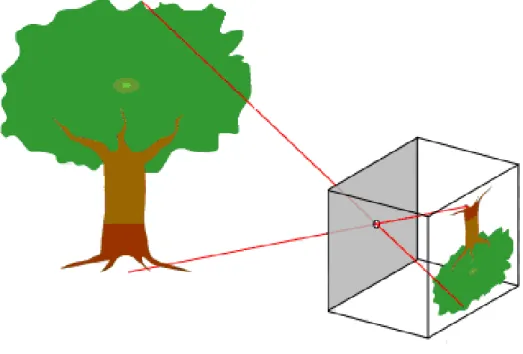
Geometry in computer vision is a sub-field in computer vision dealing with geometric relations conventionally by a pinhole camera amidst the 3D world and its projection into 2D image. The pinhole camera model illustrates the mathematical bond between the coordinates of a 3D point and its projection onto the image plane of a model pinhole camera (Hartley and Zisserman (2003). Here, the camera aperture is specified as a point and no lenses are used to focus light. For instance, the model does not comprise the geometric distortions or blurring of unfocused objects which are caused by lenses and finite sized apertures, and also does not take into account that most practical cameras have the only discrete image coordinates which means that the pinhole camera model can only be used as a first order approximation of the mapping from a 3D scene to a 2D image. Its validness depends on the quality of the camera and, generally reduces from the centre of the image to the edges as lens distortion effects increase (Forsyth and Ponce 2003).
Considering of the some effects that the pinhole camera model does not take into account can be compensated for, by applying suitable coordinate transformations on the image coordinates for instance, and other effects are adequately small to be neglected on condition that a high quality camera is performed. This implies that the pinhole camera model can usually be used as a proper description regarding how a camera depicts a 3D scene in computer vision and computer graphics, as to say.
In Figure 1.1, the geometry showing the mapping of a pinhole camera is given. Figure 1.2 shows the geometry of a pinhole camera.
Figure 1.1: A diagram of a pinhole camera Source : http://en.wikivisual.com
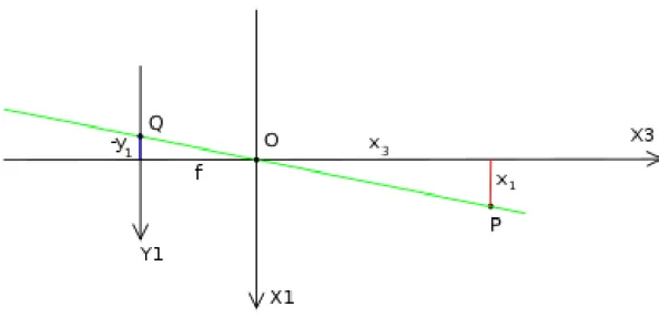
• A 3D orthogonal coordinate system with its origin at O. As well, this is where the camera aperture is placed. The three axes of the coordinate system are referred to as X1, X2, X3. Axis X3 is pointing in the viewing direction of the camera which reveals as the optical axis, principal axis, or principal ray. The 3D plane that intersects with axes X1 and X2 are the front side of the camera, or principal plane.
• An image plane where the 3D world is projected through the aperture of the camera. The image plane is parallel to axes X1 and X2 which is placed at distance f from the origin O in the negative direction of the X3 axis. An applicable implementation of a pinhole camera indicates that the image plane is located such that it intersects the X3 axis at coordinate -f where f > 0. f is also referred to as the focal length of the pinhole camera.
• The intersection of the optical axis and the image plane is marked as a point R. It is mentioned that as the principal point or image center.
• Point P can be marked at coordinate (x1, x2, and x3) relative to the axis X1, X2, and X3
on anywhere in the world.
• The projection line of point P into the camera. This green line goes through point P and point Q.
• The projection of point P is symbolized as Q, onto the image plane. It is existed by the intersection of the projection line (green) and the image plane. It can be supposed that
x3>0 which means that the intersection point is specicified nicely, in any practical
condition.
• There is exist a 2D coordinate system in the image plane, with an origin R and axes Y1 and Y2 , parallel to X1 and X2, in the order given. The coordinates of point Q related to this coordinate system is (y1, y2).
The circular hole that controls the amount of light entering a camera, as a pinhole aperture, is supposed to be eternally small, a point. In the literature, this point in 3D space is indicated as the optical (or lens or camera) center.
Let’s try to understand how the coordinates (y1, y2) of point Q depend on the coordinates
(x1, x2, x3) of point P. It is made with the help of Figure 1.3 that marks the same view as
Figure 1.2 but now from on top, looking down in negative direction of the X2 axis.
As shown in Figure 1.3, that are two similar triangles, both having parts of the projection line (green) as a hypotenuses. The catheti of the left triangle are –y1 and f and the catheti of
the right triangle are x1 and x3. These two similar triangles pursue that
3 1 1 x x fy = − or 3 1 1 x fx y =− (1.1)
A similar examination, searching in the negative direction of the X1 axis gives
3 2 2 x x fy = − or 3 2 2 x fx y =− (1.2)
This can be summarized as
which is an expression that shows the relation between the 3D coordinates (x1, x2, x3) of
point P and its image coordinates (y1, y2) given by point Q in the image plane. It should be
attention on that the mapping from 3D to 2D coordinates described by a pinhole camera is a perspective projection followed by a 180 degree rotation in the image plane. This is matched with a real pinhole camera works, the resulting image is turned 180 degree and the relative size of scheduled objects depends on their distance to the focal point and the whole size of the image depends on the distance f between the image plane and the focused point. To create an unrotated image, that it is expected from the camera, there are two alternative ways:
• In any direction, turn around the coordinate system in the image plane 180 degree. It is a solution any practical performing of a pinhole camera would fix the problem; the image is turned around before looking at it for photographic cameras, and for digital cameras pixel information is sent in such an order that it becomes rotated.
• The image plane o is put intersects the X3 axis at f instead of at –f and revise the previous calculations. This would generate a virtual (or front) image plane that can’t be carried out in practically, but provides a theoretical camera which may be simpler to analyze than the real one.
Either in these cases, the results of mapping from 3D coordinates to 2D view coordinates is given by = 2 1 3 2 1 x x x f y y (1.4)
1.2. Application Domain
Pose estimation of a 3D object with respect to a camera – or vice versa – from the object’s 2D image(s) is a subtask in robotics, computer graphics, computer and machine vision. It is, for example, used for robot guidance in manufacturing applications. In augmented reality, it is required for accurately inserting computer graphics objects into photographic scenes. In computer vision, pose estimation is instrumental for object recognition. In machine vision, it may sometimes be needed for making precise measurements. And in a variety of tasks, it is used for camera calibration (i.e., finding the pose of camera with respect to the world coordinates) before carrying out the actual task.
2. LITERATURE SURVEY
The ideas for optimizing the process of finding a pose from 2D-3D correspondences have been come up by many people. Most of the algorithms are built on a linear or nonlinear system of equations which is required to be solved, however; how these equations are obtained and how many parameters to be estimated is very different. It is not for the same purpose that all algorithms are made, it still is aimed for speed and accuracy in their area.
The hypothesize-and-test approach is the classical one to solving these coupled problems (Grimson 1990). In this approach, a small set of object feature to image feature correspondences are hypothesized, first. The pose of the object is computed, formed on these correspondences. Then, the object points are back-projected into the image using this pose. On condition that the original and back-projected images are amply similar, then the pose is accepted; or, a new hypothesis is formed and the process is repeated. The RANSAC algorithm (Fischler 1981) is perhaps the best known example of this approach, for the condition that no information is available to confine the correspondences of object points to image points. In order to determine a pose, if three correspondences are used, a high
possibility of success can be achieved by the RANSAC algorithm in ( 3log )
N MN
O time
when there are M object points and N image points.
The condition mentioned is here is one of the problems that is encountered when applying a model-based approach to the object recognition problem, and as such has taken considerable attention. (The appearance-based approach (Murase 1995) in which multiple views of the object are compared to the image is the other main approach to object recognition. Yet, as 3D models are not used, this one does not provide accurate object pose.) Many investigators (e.g., (Cass 1994, Cass 1998, Ely 1995, Jacobs 1992, Lamdan 1988, Procter 1997)) approximate the nonlinear perspective projection through linear affine approximations. This is accurate if the relative depths of object features are small compared to the distance of the object from the camera. Baird's tree-pruning method (Baird 1985), with exponential time complexity for unequal point sets, and Ullman's alignment method
(Ullman 1989) with time complexity O(N4M3logM) were among the pioneer
contributions.
The geometric hashing method (Lamdan 1988) settles an object's identity and pose, using a hashing metric computed from a set of image features. Hereby method can only be applied to planar scenes as the hashing metric must be invariant to camera viewpoint, and as there are no view-invariant image features for general 3D point sets (neither perspective nor for affine cameras) (Burns 1993).
In (DeMenthon 1993), an approach using binary search by bisection of pose boxes in 3 two 4D spaces is proposed, extending the research of (Baird 1985, Cass 1992, Breuel 1992) on affine transforms, yet; it had high-order complexity. The approach by Jurie (Jurie 1999) has been inspired for our work and is within to the same family of methods. An initial volume of pose space is guessed, and the whole correspondences compatible with this volume are first taken into account. The pose volume is then reduced again and again until it can be viewed as a single pose. Boxes of pose space are reduced not only by counting the number of correspondences that are compatible with the box as in (DeMenthon 1993), but also on the basis of the probability of having an object model in the image within the range of poses defined by the box, as a Gaussian error model is performed.
Among the researchers who have denoted the full perspective problem, Wunsch and Hirzinger (Wunsch 1996) formalize the abstract problem in a way akin to the approach advocated here as the optimization of an objective function by combining correspondence and pose constraints. Yet, the correspondence constraints are not represented analytically. Instead, each object feature is matched explicitly to the closest lines of the image features’ sight. The closest 3D points on the lines of sight are determined for each object feature, and the pose that takes the object features closest to these 3D points is chosen which allows an easier 3D to 3D pose problem to be solved. The process is reiterated until a minimum of the objective function is obtained.
The object recognition approach of Beis (Beis 1999) uses view-variant 2D image features to index 3D object models. It is performed off-line training to learn 2D feature groupings related with large numbers of views of the objects. After, the on-line recognition stage uses new feature groupings to index into a database of learned object-to-image correspondence hypotheses. These hypotheses are used for pose estimation and verification.
The pose clustering approach to model-to-image registration and the classic hypothesize-and-test approach is similar to each other. All hypotheses are created and clustered in a pose space before any back-projection and testing takes place, instead of testing each hypothesis as it is created. This former step is performed only on poses associated with high-probability clusters. It is of the idea that hypotheses including only correct correspondences should form larger clusters in pose space than hypotheses that include incorrect correspondences. Olson (Olson 1997) gives a randomized algorithm for pose
clustering with time complexityO(MN3).
Beveridge and Riseman’ method (Beveridge 1992, Beveridge 1995) is also related to DeMenthon’s approach. Random-start local search is combined with a hybrid pose estimation algorithm engaging both full/weak-perspective camera models. A steepest descent search in the space of object to-image line segment correspondences is performed. A weak-perspective pose algorithm is used to rank neighbouring points in this search space, and a full-perspective pose algorithm is used to update the object's pose after making shifting to a new set of correspondences. The time complexity of this algorithm was
determined empirically to be ( 2 2)
N M
O .
In (Kanatani, 1985b), a pose parameter estimation is proposed assuming no information on correspondences. Yet, it is assumed by the algorithm that the scene is planar with a closed curve drawn on it under orthographic projection. As the algorithm uses difference to approximate derivatives, it is generally very sensitive to noise. This algorithm has been extended in (Kanatani, 1985a) to be applicable under perspective projection.
In (Lin et al., 1986), a correspondenceless pose estimation algorithm is proposed built on the analysis of the eigenstructure of the scatter matrix.
In (Aloimonos and Herve, 1990), it is a correspondenceless pure translational pose estimation algorithm is proposed which assumes that the z component of the translation vector is much smaller than the depth of the scene. As a result, the author approximates as equal the depths of the same 3D point in different camera centred coordinate frames.
In (Lin et al., 1994), a correspondenceless pose estimation algorithm under orthographic projection is proposed. Three cameras are used by the algorithm and it is based on the eigenstructure analysis of the scatter matrix.
In (Govindu et al. 1998), a correspondenceless pose estimation has been proposed based on the use of the geometric descriptors of a contour. In the experiments, aerial images are used where the 2D contour may be extracted. However, the transformation cannot be guaranteed to be a 2D transformation, so that the usefulness of the algorithm is severely limited.
In (Tarel et al., 1997), a correspondenceless method was proposed to estimate 3D projective transformation parameters. This algorithm uses an iterative method to find the initial estimation first for projective transformation parameters based on bitangent lines and bitangent planes. Then the pose parameters are refining by iteration based on the extended ICP (Iterative Closest Point) algorithm.
In Liu and Rodrigues (2001), a correspondenceless pose estimation algorithm has been induced from a realistic camera setup. The algorithm provides a closed form solution to all parameters of interest. What is important to emphasize is that the algorithm does not require disambiguating multiple solutions which is in contrast with some correspondence-based and correspondenceless pose estimation algorithms (e.g. Fishler and Bolles, 1981; Tsai and Huang, 1984; Lin et al., 1986, 1994; Huang and Netravali, 1994; Tarel et al., 1997).
3. FEATURE EXTRACTION
GPE needs the coordinates of the points that determined as the points of the object model. To give this information to the GPE a feature extraction must be done on the picture.
3.1. MANUAL, SEMI-MANUAL, AND AUTOMATED FEATURE EXTRACTION
The manual method is the basic method to get the coordinates is using a tool that gives the pixel coordinates and then typing the coordinate to the file which GPE uses it as an input. This method is very simple but it is not useful in terms of time and accuracy.
In semi-manual method, a program should be used to do the job. The program takes the picture as an input and shows it on the screen. When the user clicks mouse on an area in the picture the program writes the coordinates of the pixel to the file that GPE uses.
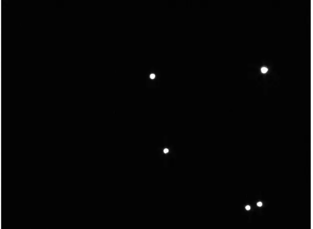
The most useful method is to automate all the steps. The points on the object that is used for object model are marked by infrared leds. Also an infrared filter is used on the camera which the pictures are taken by. After these, the picture is taken. As shown in Figure 3.1 there can be seen only black and white areas. White regions are formed by the infrared leds and also these regions are points that are needed for GPE. However, there must be an algorithm which is called blob coloring or contour tracing to to make the white regions meaningful. Using the blob coloring algorithm the centers of mass of the white regions can be find. Finally these parameters can be used by GPE as input.
3.2. TRADE-OFFS IN BLOB COLORING
Blob coloring scans an image and groups its pixels into blobs based on pixel connectivity,
i.e. all pixels in a blob share similar pixel intensity values and are in some way connected
with each other. It can be seen in Figure 3.2 briefly. Once all groups have been determined, each pixel is labeled with a graylevel or a color (color labeling) according to the blob it was assigned to.
Extracting and labeling of various disjoint and connected blobs in an image is central to many automated image analysis applications. The applications use several algorithms. The efficiency of these algorithms are appears in big images or complex images. There are six algorithms explained in below. The most efficient one in literature is Main Color Emphasized Blob Coloring Algorithm. Because it scans the whole image only once. In contrast, the other algorithms have to scan the image twice.
3.2.1. Rosenfeld and Pfaltz’s Algorithm
The first method which is suggested by Rosenfeld and Pfaltz carries out two passes over a binary image. Each point is encountered once in the first pass. A further study of its four neighbouring points (left, upper left, top, and upper right) is conducted at each black pixel P. If none of these neighbours carries a label, then P is allocated a new label. In other ways, those labels carried by neighbours of P are said to be equivalent. In this occasion, the label of P is replaced by the minimal equivalent label. For this resolution, a pair of arrays; one containing all current labels and the other the minimal equivalent labels of those current labels, is generated,. In the second pass, label substitutes are made.
Figure 3.2 : L-shaped template for blob coloring
3.2.2. Haralick’s Algorithm
Haralick designed a method to remove the excess storage required for the pair of arrays which are suggested in the first method. Each black pixel is given a unique label, first. The labelled image is then processed iteratively in two directions. Each labelled point is reassigned the smallest label among its four neighbouring points in the first pass, administered from the top down,. The second pass is similar to the first, except that it is administered from the bottom up. The process goes on iteratively until no more labels change. The memory storage of hereby method is small, yet; the overall processing time differs according to the complexity of the image being processed.
3.2.3. Lumia’s Algorithm
In the method put up by Lumia et al. which compromises between the two preceding methods, labels are assigned to black pixels in the first top-down pass as in the first method. However, the labels on this line are adjusted to their minimal equivalent labels at the end of each scan line,. The second pass begins from the bottom and works similarly as the top-down pass which can be proven that all components obtain a unique label after these two passes.
3.2.4. Fiorio and Gustedt’s Algorithm
A special model of the union-find algorithm was activated by Fiorio and Gustedt, that it runs in linear time for the component-labeling problem. This methodology is made up of two passes. In first one, each set of corresponded labels is described as a tree. And a re-labeling progress is performed in the second pass. To combine two trees into a single tree, this operation is used in the union-find methods serves, when a node in one tree bears an 8-connectivity relations to a node in the other tree.
3.2.5. Shima’s Algorithm
Shima offered this method et a1. is specifically fit for compressed images in which a procedure before processing as required to reform image elements into runs. An examining part and a propagation step are practiced frequently on the run data. In the examination part, the image is countered till an unlabeled run (referred as a focal run) is found and is allocated a new label. In the propagation step, the label of each focal run is produced to adjacent runs above or below the scan line.
3.2.6. Main Color Emphasized Blob Coloring
Main Color Emphasized Blob Coloring Algorithm (MCEBC) quantizes the colors into the predefined color classes, using the heuristic information that humans tend to emphasize the dominant color component when they perceive and memorize colors. The experimental results indicate that the method approximates the user's classification better than the other methods that use the mathematical color difference formulas. The MCEBC algorithm is implemented in a content-based image retrieval system, called QBM system. The retrieval results of the system using MCEBC algorithm is quite satisfactory and shows higher success rates than using other methods.
3.2.6. Proposed Blob Coloring Algorithm
There are six major algorithms in literature. The most efficient of them is the MCEBC algorithm. However, using simple images it is not needed to use the MCEBC. In addition to this, in the next section it has been seen that in simple images, Rosenfeld and Pfaltz’s algorithm is relatively faster than MCEBC. So Rosenfeld and Pfaltz’s algorithm is used in the blob coloring part of the thesis. The algorithm can be seen below.
Let the initial color, k=1. Scan the image from left to right and top to bottom. If f(xC) =0 then continue
else
begin
if (f(xL) =1 and f(xU) =0)
then color (xC): = color (xL)
if (f(xL) =1 and f(xU) =1) then begin
color (xC): = color (xL)
color (xL) is equivalent to color (xU)
end
comment: two colors are equivalent.
If(f(xL) =0 and f(xU) =0)
then color (xC): = k; k:=k+1
comment: new color end
3.2.7. Blob Coloring Results
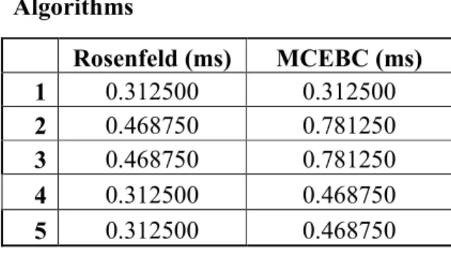
As always done there should be choosen a method to do the blob coloring efficiently. To make this Rosenfeld and Pfaltz’s algorithm and MCEBC are tested with same photos. As it was told above, the MCEBC algorithm is the best blob coloring algorithm in literature. However, because of using the infrared leds and infrared filters, the taken photos become simpler. This reason effects the run-times positively especially the Rosenfeld and Pflatz method. In Table 3.1 the run-time results can be seen. Two of the methods find the blobs very quickly.
Rosenfeld (ms) MCEBC (ms)
1 0.312500 0.312500
2 0.468750 0.781250
3 0.468750 0.781250
TABLE 3.1 Results of Blob Coloring Algorithms
4. GRAVITATIONAL POSE ESTIMATION
Gravitational Pose Estimation (GPE) is a correspondenceless method which is inspired by classical mechanics. GPE can handle occlusion and uses only one image (i.e., perspective projection). GPE creates a simulated gravitational field from the image and lets the object model move and rotate in that force field, starting from an initial pose.
4.1. PROBLEM FORMULATION
Image of a 3D point (on the image sensor of a regular camera) is the perspective projection of the point on to the image plane – though less accurate approximations (e.g. orthographic projection) are possible. If the coordinates of the point are ( , , )x y z with respect to the
camera coordinate frame (origin is the camera lens’ center and the X-Y axes are along the edges of the rectangular image sensor), then its image is located at ( . / , . / , )x f z y f z f where
f is the distance between the camera lens and image plane – called f because it is approximately equal to the focal length of the lens. In real life, image plane is behind the camera lens at z= −f and image is inverted. However, most treat it as if the image plane is at z= f without any loss of generality – a simple flip of all three coordinates does the job. All points on line(kx ky kz, , ), where k is a free parameter, produce the same image point on
the image plane. Therefore, for each image point, it can be constructed a unique line in 3D (called line of sight) on which the object point must be located.
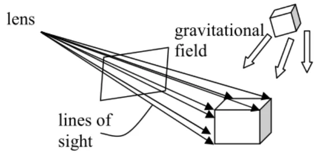
A camera image does not consist of feature points; instead it consists of pixels, each of which is assigned a value indicating brightness and color if any. However, it is possible to transform an image to a collection of feature points by computer vision techniques. Each of the feature points on the image plane corresponds to a point on the object and gives us a line of sight (LOS) in 3D when extended through the lens center. Thus, from the image of an object a pencil of lines is obtained, and it is known that they go through the object as in Figure 4.1.
GPE (and similar techniques) require a rigid object model, which is a set of 3D object
points (i.e., feature points) expressed by their coordinates in the object coordinate frame.
Then, the answer to the pose estimation problem is the pose where the object points are as close to the LOSes as possible. From the above discussion an energy function can be devised, which is expected to be zero when the correct pose is found. Below are the steps to calculate the energy of a suggested pose for the object:
• For the suggested pose, transform object points’ coordinates in the object model from the object coordinate frame to the camera coordinate frame. (Everything from this point on is computed in the camera coordinate frame.)
• Construct the LOSes from the image points.
• Let dij be the shortest, hence perpendicular distance, between the ith point of the object model and the jth LOS. Calculate and sort all dij’s in ascending order. Place them in a
list called DistanceList.
• Pair the LOSes with object points until there is no LOS left (assuming no false feature points). Do this in such a way that an object point is paired with only one LOS
Figure 4.1: An object in the gravitational field of the lines of sight
Source : H. Fatih Ugurdag, Sezer Gören and Ferhat Canbay, 2008. Correspondenceless pose estimation from a single 2D image using classical mechanics. October 2008. gravitational field lines of sight lens
element in DistanceList), and assign the ith point of the object model to the jthLOS.
Erase all distances in DistanceList that belong to object point i (all dik where k is a free
parameter) as well as all distances that belong to LOS j (all dkj where k is free).
Continue with the smallest dmn in the updated DistanceList, and pair object point m and
LOS n. Continue until all LOSes are paired.
• Calculate the energy of object model in the suggested pose, which is equal to the sum of squares of the distances between all LOS-object point pairs:
2 ij
E=
∑
d (4.1)It should be noted that one can calculate the average distance between the points and lines as in:
( /# lines) ave
d = E (4.2)
When the estimated (suggested) pose is equal to the correct pose, dave should be quite small
with respect to the dimensions of the object. Although this is currently our criterion, a maximum feature distance criterion may also be imposed.
4.2. OVERALL APPROACH
The algorithm starts by forming the LOSes. A line can be represented (though not canonically) by a point on it and a (unit-length) direction vector. As the object points are wanted to coincide with the LOSes, it is quite intuitive to form a gravitational field where LOSes attract object points as shown in Figure 4.1. Since is not wanted object points to move after they reach the LOSes, it makes sense to make the force (gravitational field) proportional to the distance between object points and LOSes. The outline of the algorithm is as follows:
energy calculation instructions.
2) Calculate the force on each object point through equation (4.3), where fi r
is the force on
object point i and dij is the distance between the i th
object point and its paired LOS j,
and rˆij is the unit vector that points from point i to line j and is perpendicular to line
. j ˆ i ij ij f =d r r (4.3)
3) Use classical mechanics to calculate the translational, at r
, and rotational acceleration,
r
ar , as follows:
a) Calculate effective force, fcm r
applied to the object’s center of mass (COM) by:
. cm i i f =
∑
f r r (4.4)Note that force on an unpaired object point (a possibly occluded point) is zero. However, unpaired points still contribute to the COM calculations, i.e., they are still considered part of the object.
b) Calculate translational acceleration, at r
, which is the acceleration of object’s COM,
by (4.5), where mtot is the total mass of the object. (Normally, it is assumed every
feature point has a mass of 1. However, if there are different degrees of certainty in feature extraction or there are reasons to believe that some feature points have to be aligned more carefully with LOSes, then those points may be assigned a larger mass than other points.)
/ t cm tot a = f m r r (4.5)
c) Calculate total torque, tcm r
, around the COM using the summation of cross-products
in (4.6), where (rcm i) r
is the vector that gives the relative displacement of point iwith
respect to COM. ( ) cm cm i i i t =
∑
r × f r r r (4.6)d) Calculate the rotational inertia matrix of the object (at the current pose,) R, through (4.7), where ( )R pq is a component of matrix R that is located in row p and column
q, mi is the mass of object point i, and ((rrcm i k) ) , ((rrcm i) ) , and ((p rrcm i q) ) denote the
kth, pth, and qth components of the vector (rcm i) r respectively. ( pq i {((cm i k) ) ((cm i k) ) ((cm i) ) ((p cm i q) ) } i k m r r r r =
∑ ∑
− R) r r r r (4.7)e) Calculate angular acceleration, arr, using (4.8), where −1
R is the inverse of rotational inertia matrix, R.
1
r cm
ar =R−tr (4.8)
4) Let the pose of object be expressed by vectors n s ar r, , r (unit vectors by definition) and
p
r
, where nr is the orientation of X-axis of the object model (object coordinate frame)
expressed in the camera coordinate frame, sr is the orientation of Y-axis, ar is the orientation of Z-axis, and pr is the position of object. Then:
a) Calculate ∆pr where ∆ =p at r r
and ∆pr is the change in pr, so add ∆pr to old pr to get the new pr.
b) Rotate n sr r, , and ar around the vector ar r
by an angle equal to ar r
radians, where ar r
denotes the length of the vector ar. r
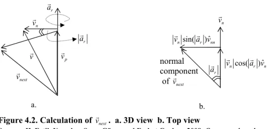
In order to do this, we follow the steps below
Let vr be a vector to be rotated around ar r
shown as in Figure 4.2. Normalize vr (i.e., make it
unit-length) to get unit vector vˆ. Identify the two components of vˆ., vˆpand vˆn, where vˆp is
parallel to ar r
, and vˆn is normal (i.e., perpendicular) to ar r
, using normalization, dot-product,
and scalar multiplication in (4.9) and vector subtraction (4.10).
ˆ ˆ ˆ ( . ) p r r vr = a v a (4.9) n p vr = −vr vr (4.10)
i) Construct unit vector vˆnn from vˆn using (4.11). Vector vˆnn is normal to plane vˆn
and ar r
, and is the direction vector vr moves when it is rotated around ar r
.
ˆ ˆ
nn r n
vr =a ×v (4.11)
ii) Calculate the next vr denoted as vnext r using (4.12): = + + r r r r r next vr vr r ar p vr n vr r ar n vr ˆ cos( ) n r n vr a vr ˆ sin( ) n r nn vr a vr normal component of vnext r a. b.
Figure 4.2. Calculation of vnext r
. a. 3D view b. Top view
Source : H. Fatih Ugurdag, Sezer Gören and Ferhat Canbay, 2008. Correspondenceless pose estimation from a single 2D image using classical mechanics. October 2008.
r
5) Calculate the energy E at the next pose – pair object points and LOSes – use (4.1). If the energy obtained is not small enough, go to step 2 and continue to move the object in the gravitational field until it gets stuck in a locally minimum energy state. If it is stuck, then update the minimum pose and energy, provided current one is the best. If the energy is still not small enough (and the maximum number of iterations is not reached,) then go to step 6 to shake the object (shake means a random rotation).
6) Generate an angular acceleration, ar, r
randomly. Apply step 4 to calculate the next
orientation. Then go to step 1.
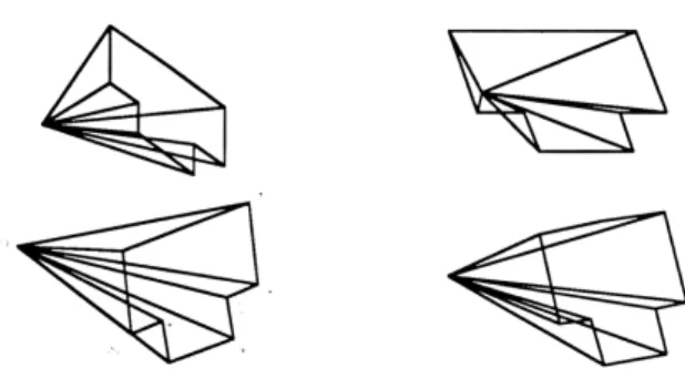
As an example, a 10-point object is shown in Figure 4.3. GPE has been run by taking the true pose as
(1,0,0), (0,1,0), (0, 0,1), (0, 0,5)
nr= sr= ar= pr=
and initial pose as
(0,1,0), (0,0,1), (1,0,0), (20, 20, 20).
nr= sr= ar= pr=
Figure 4.3: Four different views of a 10-point synthetic object (3 of the points are collinear)
Source : H. Fatih Ugurdag, Sezer Gören and Ferhat Canbay, 2008. Correspondenceless pose estimation from a single 2D image using classical mechanics. October 2008.
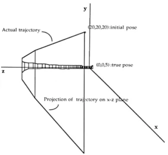
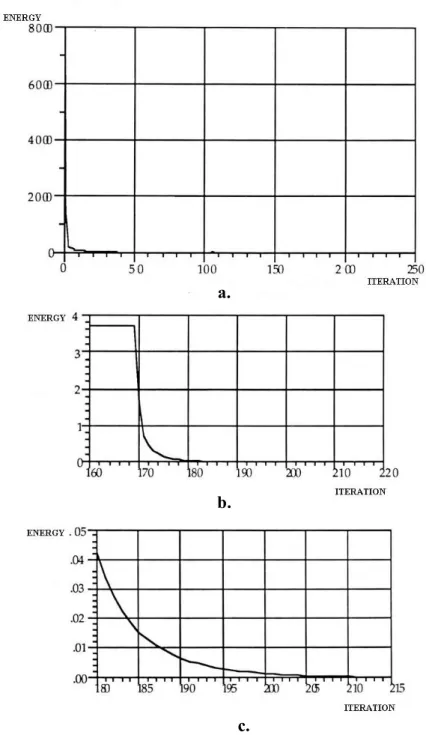
The initial energy came out to be around 8,000. The criterion for a local minimum was set such that the absolute change in the energy is less than 0.0001 for 30 consecutive iterations. The criterion for termination was either getting an energy of less than 0.0002 or to reaching iteration 1,000. (For our larger set of experiments, it has been used up to 50,000 iterations since GPE runs quite fast.) The result of this initial experiment was impressive. The number of shakes was only 2. The program stopped with energy less than 0.0002 after the 215th iteration. The trajectory of the object during the program execution is plotted in Figure 4.4. In addition, energy versus iteration count is given in Figure 4.5.
Figure 4.4: Trajectory of the above object during GPE’s search for the true pose.
Source : H. Fatih Ugurdag, Sezer Gören and Ferhat Canbay, 2008. Correspondenceless pose estimation from a single 2D image using classical mechanics. October 2008.
Figure 4.5: Energy versus iterations
a. Overall plot. b. Zoomed in near the last shake. c. Final slope.
Source : H. Fatih Ugurdag, Sezer Gören and Ferhat Canbay, 2008. Correspondenceless pose estimation from a single 2D image using classical mechanics. October 2008.
a.
b.
4.3. GPESoftPOSIT
GPEsoftPOSIT is an integration of the two algorithms, GPE and SoftPOSIT. The main idea here is to run SoftPOSIT with an initial guess that is close to the true pose instead of trying any random starts. The pose found by GPE is taken as the initial guess for the object’s when running SoftPOSIT. Whenever the ratio of object points matched to LOSes to the total number of object points reaches a predetermined criterion (here it is set to 0.7) and also SoftPOSIT satisfies its own definition of convergence, then SoftPOSIT terminates and outputs the guess for the object’s pose. If SoftPOSIT is unable to find a pose, then the initial guess for the object’s pose (the result of GPE) is presented as the output.
SoftPOSIT has a parameter, calledβ0, which corresponds to the fuzziness of the
correspondence matrix. If the initial pose is close to the actual pose, then β0 should be
around 0.1. In our case, since our initial pose comes from GPE and it is known that it is close to the actual pose, it is set β0 to 0.1. As an exercise, the 10-point synthetic object in
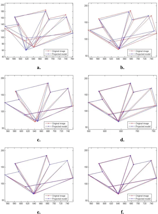
Figure 4.3 and its image for a given pose were constructed. Using the object model and image, GPE was run and its result was piped to SoftPOSIT. The projected model and the original image are shown in blue and red, respectively in Figure 4.6a through 4.6e. The projected model shown in Figure 4.6a corresponds to the object at the pose found by GPE. The iterations of SoftPOSIT, on the other hand, are shown in Figure 4.6b through 4.6e.
Figure 4.6: Converging to optimum using GPEsoftPOSIT. a. Object at the pose found by GPE has been projected to the image plane.
b. c. d. e. f. Iterations of SoftPOSIT to improve the pose.
a. b.
c. d.
4.4. TRADE-OFFS IN POINT-LINE MATCHING
The most important part of the GPE algorithm is the matching the points with lines accurately. Key point is the distances between point and lines. If the total value of the distances after matching equals zero, the perfect matching is found. However, in real life this result can not be found zero. So the results are approximately zero. There are various type of algorithms to match points and lines but two of them are compared and better one is used.
4.4.1. Regular Method
In this method a matrix is used to for the distances between points and lines. In addition to this, two lists are used for the unmatched points and lines. And also an array is used for matched items as matching table. Let’s call for unmatched points Ind_P, for unmatched lines Ind_L, for the matching table A and the distances between points and lines will be hold in matrix M.
• The algorithm finds the minimum distance in M and keeps the index of it. While scaning the M the algorithm looks for the unmatched index using Ind_P and Ind _L. • After finding the minimum value, the algorithm deletes the index value of matched
point and line from Ind_P and Ind_L and keeps the values in A.
• The index of A is used for lines and the value in this index is used for index of point. This process ends when Ind_P becomes empty.
As in the below, algorithm simulated on four points and four lines. The initial values used in algorithm can be seen in Figure 4.7.
The first step of the algorithm can be seen in Figure 4.8. Minimum distance is found in index L0-P3 of matrix M and this matching is assigned on A. After these, L0 is deleted from Ind_L and P3 is deleted from Ind_P.
In the second step of the algorithm, the minimum value is searched in a smaller part of the M. In Figure 4.9 it is shown using coloring. Gray colored cells are matched in previous step and the white cells are available for searching. After searching the available points and lines it is found that the minimum distance is in the index P1-L1. 1 is recorded in index 1 of A. P1 is removed from Ind_P and L1 is removed from L1.
P0 P1 P2 P3 L0 1 5 2 0 L1 3 0 1 4 L2 2 1 0 3 L3 0 1 2 3 0 1 2 3 Ind_P = { 0, 1, 2 , 3 } Ind_L = { 0, 1, 2, 3 }
Figure 4.7 : The initial values of the elements before the algorithm starts
M A
P0 P1 P2 P3 L0 1 5 2 0 L1 3 0 1 4 L2 2 1 0 3 L3 0 1 2 3 0 1 2 3 3 1 Min = L1, P1 Ind_P = { 0, 1, 2 } Ind_L = { 1, 2, 3 }
Figure 4.9: Second Step of the Algorithm
Matrix M A P0 P1 P2 P3 L0 1 5 2 0 L1 3 0 1 4 L2 2 1 0 3 L3 0 1 2 3 0 1 2 3 3 Min = L0,P3 Ind_P = { 0, 1, 2, 3 } Ind_L = { 0, 1, 2, 3 }
Figure 4.8: First Step of the Algorithm
Matrix M A
After searching the M, the minimum value is found in L2-P2. Again, doing same processes above, P2 and L2 are matched and they are removed from the available ones as shown in
P0 P1 P2 P3 L0 1 5 2 0 L1 3 0 1 4 L2 2 1 0 3 L3 0 1 2 3 0 1 2 3 3 1 2 0 Min = L1, P1 Ind_P = { 0 } Ind_L = { 3 }
Figure 4.11 : The situation of the elements after the algorithm runs Matrix M Matched P-L P0 P1 P2 P3 L0 1 5 2 0 L1 3 0 1 4 L2 2 1 0 3 L3 0 1 2 3 0 1 2 3 3 1 2 Min = L1, P1 Ind_P = { 0, 2 } Ind_L = { 2, 3 }
Figure 4.10 : Third Step of the Algorithm
Matrix M Matched P-L
As it can be seen in Figure 4.11 last step of the algorithm is the simplest step. Because there is only one point and one line. They are matched without searching and matching table is filled fully.
4.4.2 Sorting Based Method
In the sorting based method two one-dimensional arrays are used instead of a matrix. First one is used to keep the Line-Point information (LP) and the second one is used to keep the distances (D).
• The algorithm begins with sorting the second array smaller to the greater distance. When a swap process is done, the same process is done on array LP too.
• After sorting the arrays the first element of the arrays are match to each other and the matched line and point’s indicies are marked.
• In the other steps it matches the first unmarked point-line and marks the indicies that these point and line have. The algorithm is simulated below.
As shown in Figure 4.12, values of the matrix used in regular method is also used in sorting based method. The values are inserted to the one-dimensional array row by row.
P0 P1 P2 P3 L0 1 5 2 0 L1 3 0 1 4 L2 2 1 0 3 L3 0 1 2 3 L0 -P 0 L0 -P 1 L0 -P 2 L0 -P 3 L1 -P 0 L1 -P 1 L1 -P 2 L1 -P 3 L2 -P 0 L2 -P 1 L2 -P 2 L2 -P 3 L3 -P 0 L3 -P 1 L3 -P 2 L3 -P 3 1 5 2 0 3 0 1 4 2 1 0 3 0 1 2 3 0 1 2 3 M LP D A
In the first step array D is sorted from smaller to bigger. As it can be seen in Figure 4.13, array LP changes at the same time D.
The algorithm starts to match the points and lines by the end of sorting step. The first element of the array D is the minimum. So it is matched to each other and its background is colored red in Figure 4.14. The zero index of A is assigned 3, because of being matched with P3. L0 -P 3 L1 -P 1 L2 -P 2 L3 -P 0 L0 -P 0 L1 -P 2 L2 -P 1 L3 -P 1 L0 -P 2 L2 -P 0 L3 -P 2 L1 -P 0 L2 -P 3 L3 -P 3 L1 -P 3 L0 -P 1 0 0 0 0 1 1 1 1 2 2 2 3 3 3 4 5 0 1 2 3 LP D A Figure 4.13 : First Step of the Algorithm
In the second step L0 and P3 were matched. In Figure 4.15 the background of the related elements of array LP and D are colored gray. The algorithm finds the first uncolored element. It is the second element of D and L1 and P1 are matched with each other. Its background is colored red in Figure 4.15 like the second step. After these, P1 is written on index one of the array A.
L0 -P 3 L1 -P 1 L2 -P 2 L3 -P 0 L0 -P 0 L1 -P 2 L2 -P 1 L3 -P 1 L0 -P 2 L2 -P 0 L3 -P 2 L1 -P 0 L2 -P 3 L3 -P 3 L1 -P 3 L0 -P 1 0 0 0 0 1 1 1 1 2 2 2 3 3 3 4 5 0 1 2 3 3 LP D A Figure 4.14 : Second Step of the Algorithm
As shown in Figure 4.16 the new minimum value is the third element of array D and LP which keep L2 and P2.
L0 -P 3 L1 -P 1 L2 -P 2 L3 -P 0 L0 -P 0 L1 -P 2 L2 -P 1 L3 -P 1 L0 -P 2 L2 -P 0 L3 -P 2 L1 -P 0 L2 -P 3 L3 -P 3 L1 -P 3 L0 -P 1 0 0 0 0 1 1 1 1 2 2 2 3 3 3 4 5 0 1 2 3 3 1 LP D A Figure 4.15 : Third Step of the Algorithm
In the last step there there is only one uncolored element exists in array LP and D. As it is seen Figure 4.17, this element is the fourth one. L3 and P0 are matched and all of the lines and points are matched by the end of this step.
L0 -P 3 L1 -P 1 L2 -P 2 L3 -P 0 L0 -P 0 L1 -P 2 L2 -P 1 L3 -P 1 L0 -P 2 L2 -P 0 L3 -P 2 L1 -P 0 L2 -P 3 L3 -P 3 L1 -P 3 L0 -P 1 0 0 0 0 1 1 1 1 2 2 2 3 3 3 4 5 0 1 2 3 3 1 2 LP D A
4.4.3. Point-Line Matching Results
There were used two different point-line matching algorithm which are called regular method and sorted-based. For comparing the two algorithms six different data fed as input to algorithms. Number of points and lines feeded from smaller to greater. As it can be seen in Table 4.1 below they finds the results in the same time when the data is smaller. Hovewer, when the data become bigger the regular method gets the result faster. Also in Figure 4.18, runtimes are shown on a graphic.
L0 -P 3 L1 -P 1 L2 -P 2 L3 -P 0 L0 -P 0 L1 -P 2 L2 -P 1 L3 -P 1 L0 -P 2 L2 -P 0 L3 -P 2 L1 -P 0 L2 -P 3 L3 -P 3 L1 -P 3 L0 -P 1 0 0 0 0 1 1 1 1 2 2 2 3 3 3 4 5 0 1 2 3 3 1 2 0 LP D A Figure 4.17 : Last Step of the Algorithm
Number of Points-Lines Regular Method (ms) Sorting Based Method (ms) 10 0 0 20 15.6250 15.6250 40 31.2500 31.2500 100 171.8750 406.2500 150 390.6250 593.7500 200 718.7500 1156.2500
TABLE 4.1 : Runtime comparison of the point-line matching algorithms 0 200 400 600 800 1000 1200 1400 10 20 40 100 150 200 Number of Points T im e (m s ) _ Regular Sorted
Figure 4.18: Performance graphic of the Regular and Sorting Based matching algorithms
5. GRAVITATIONAL POSE ESTIMATION EXPERIMENTS
GPE has been first validated using real images, and then GPE, GPEsoftPOSIT, and random start SoftPOSIT has been compared on synthetic data with and without occlusion.
5.1. RESULTS WITH REAL IMAGES
In this section, GPE is tested (without SoftPOSIT) with real images taken by a simple webcam, and our results are still impressive. (A webcam or any other cheap camera has a fish-eye effect. Please notice that the A4 paper’s borders in Figure 5.1 look curved.) There is a fixture used in experiments (see Figure 5.2) where an object can be attached, rotate the object by means of an arm, and adjust the angle manually. As there is a protractor attached to the arm, it is exactly known what the actual angle is. In Figure 5.1, the images of a black polygon are taken when the object is brought to angles 70°, 75°, 80°, 85°, 90°, 95°, 100°, 105°, and 110° on the protractor. All of the images taken are shown in Figure 5.1a through 5.1i.
Although GPE can measure all 6 degrees of freedom of a 3D pose, it is hard to measure the same 6 degrees of freedom mechanically as it requires a very fancy apparatus. Instead there is a simple mechanical fixture where it can be measured one degree of freedom (a rotation angle) with great precision. From GPE it is received two 3D poses and compare them to find the rotation angle and then compare it with the angle read from the fixture’s protractor. Note that the plane that the arm traverses when rotated (i.e., the plane of the protractor) and plane of the A4 sheet (where the polygon is drawn) are the same.
Figure 5.1 : Images of a real object taken at various angles: a. 70o b. 75 o c. 80 o d. 85 o e. 90 o f. 95 o g. 100 o h. 105 o i. 110 o
Source : H. Fatih Ugurdag, Sezer Gören and Ferhat Canbay, 2008. Correspondenceless pose estimation from a single 2D image using classical mechanics. October 2008.
a. b. c.
d. e. f.
In the real image experiment, the object model contains corners of the polygon. The feature extraction has been done manually by pointing to the corners of the polygon with the mouse and reading the coordinates by means of image viewing software. The object coordinate frame is defined by the A4 sheet. The Z-axis is orthogonal to the sheet and the X and Y axes are along the edges of the sheet. The directions of the X, Y, Z axes of the object model are expressed respectively by n sr r, , and ar in the camera coordinate frame.
To evaluate the accuracy of GPE, the relative angle between every image pair was measured by both GPE and protractor. The results of this experiment are given as a chart in Figure 5.3. In the chart, ACTUAL2 (horizontal) axis denotes the angle value for image 2, whereas the numbers next to word “vs” denotes the protractor angle for image 1. After running GPE twice, the difference between the two angles is computed. ESTIMATED2 (vertical) axis in Figure 5.3 is the angle estimated for image 2 by GPE. That is, in fact, the difference estimated by two runs of GPE (θ ) plus the angle of image 1 from the protractor.
8 groups of image pairs are included in Figure 5.3:
vs 70: Image 1 at 70o versus image 2 at {75o, 80o, 85o, 90o, 95o, 100o, 105o, 110o }.
Figure 5.2 : The fixture used for the real image experiment
vs 85: Image 1 at 85o versus image 2 at {90o, 95o, 100o, 105o, 110o }. vs 90: Image 1 at 90o versus image 2 at {95o, 100o, 105o, 110o }. vs 95: Image 1 at 95o versus image 2 at {100o, 105o, 110o }. vs 100: Image 1 at 100o versus image 2 at {105o, 110o }. vs 105: Image 1 at 105o versus image 2 at 110o.
Figure 5.3 : Estimation of relative angle of the object between two image pairs of Figure 5.1
Source : H. Fatih Ugurdag, Sezer Gören and Ferhat Canbay, 2008. Correspondenceless pose estimation from a single 2D image using classical mechanics. October 2008.
Absolute estimation error (GPE minus protractor) is presented in Figure 5.4 in degrees. The average absolute error for the 36 image pairs is 0.43o. Table 5.1 is also presented where the run-time of the pose estimation algorithm and the number of shakes for the 8 experiments
Figure 5.4 : Absolute error in estimated relative angle in Figure 5.3
Source : H. Fatih Ugurdag, Sezer Gören and Ferhat Canbay, 2008. Correspondenceless pose estimation from a single 2D image using classical mechanics. October 2008.
TABLE 5.1 : Performance of pose
estimation algorithm
Image Number of Shakes Run-time (s)
75o 69 12.6 80o 97 15.2 85o 104 8.3 90o 99 7.9 95o 71 9.6 100o 69 22.1 105o 60 15.6 110o 63 21.3
Source : H. Fatih Ugurdag, Sezer Gören and Ferhat Canbay, 2008. Correspondenceless pose estimation from a single 2D image using classical mechanics. October 2008.