A visiual isarithmic mapping tool for online maps

M.Sc. THESIS

JANUARY 2018

A VISUAL ISARITHMIC MAPPING TOOL FOR ONLINE MAPS

Thesis Advisor: Assist. Prof. Dr. Osman Sami KIRTILOĞLU Hatice ATALAY

Department of Geomatics Engineering IZMIR KATIP CELEBI UNIVERSITY

Department of Geomatics Engineering

JANUARY 2018

A VISUAL ISARITHMIC MAPPING TOOL FOR ONLINE MAPS

M.Sc. THESIS Hatice ATALAY

(Y140108008)

Thesis Advisor: Assist. Prof. Dr. Osman Sami KIRTILĞLU IZMIR KATIP CELEBI UNIVERSITY

Harita Mühendisliği Anabilim Dalı

OCAK 2018

İZMİR KÂTİP ÇELEBİ ÜNİVERSİTESİ  FEN BİLİMLERİ ENSTİTÜSÜ

ONLİNE HARİTALAR İÇİN GÖRSEL İZARİTMİK HARİTALAMA ARACI

YÜKSEK LİSANS TEZİ Hatice ATALAY

(Y140108008)

vii

ix FOREWORD

Firstly I would like to thank to my advisor, Assist. Prof. Dr. Osman Sami Kırtıloğlu. I highly appreciate my Linkedin connection Mürsel Öztürk who is a second advisor to me. I would like to thank my friends Nilay Küçükdoğan Öztürk, Melike Karakaya and Fatma Günseli Yaşar for guiding me with their experiences and for their precious support.

xi TABLE OF CONTENTS Page FOREWORD ... ix TABLE OF CONTENTS ... xi SYMBOLS ...xiv LIST OF FIGURES ... xv SUMMARY ...xvi ÖZET ………xvi i INTRODUCTION ...1 1. Literature Review and Objects of the Thesis ... 1

1.1 THEMATIC MAPPING AND INTERPOLATION METHODS ...8

2. Thematic Maps ... 8

2.1 Spatial Interpolation Methods ...13

2.2 2.2.1 Non-Geostatistical Interpolators ... 13

2.2.1.1 Nearest Neighbours...13

2.2.1.2 Triangulated Irregular Network ...14

2.2.1.3 Natural Neighbours Method ...22

2.2.1.4 Inverse Distance Weighting Method ...23

2.2.1.5 Regression Models...24

2.2.1.6 Trend Surface Analysis ...24

2.2.1.7 Splines and Local Trend Surfaces ...25

2.2.1.8 Other Methods ...26

2.2.2 Geostatistical Interpolators ... 26

A VISUAL ISARITHMIC MAPPING TOOL ... 29

3. Material and Method ...29

3.1 Thematic Mapping ...31 3.2 3.2.1 IDW Interpolation ... 32 3.2.2 Kriging Interpolation ... 33 3.2.3 TIN Interpolation ... 35

RESULTS AND CONCLUSIONS ... 37

4. DISCUSSION and FUTURE STUDIES... 38

5. REFERENCES ... 39

APPENDICES ... 42

APPENDIX A ...43

xiii ABBREVIATIONS

ANN : Artificial Neural Network API : Application Program Interface CSS : Cascading Style Sheets

DEM : Digital Elevation Model

GIS : Geographic Information Systems HTML : Hypertext Markup Language HTTP : Hyper Text Transfer Protocol IDW : Inverse Distance Weighting LTS : Local Trend Surfaces

OGC : Open Geospatial Consortium OSM : Open Street Map

WMS : Web Map Service

SIM : Spatial Interpolation Method TIN : Triangulated Irregular Network

xiv SYMBOLS

̂ : Estimated value of the variable at the point of interest z : Observed value at the sampled point x_i

: Weight of the sampled point n : The number of sampled points

, : Coordinate Values

: Each neighbour’s area : The weights

p : Power Parameter

: Function defining the sample points

: Three-dimensional spatial distance between the sampling points and the point to be interpolated

xv LIST OF FIGURES

Page Dot Density Map ...9 Figure 2.1 :

Isoline Map ... 10 Figure 2.2 :

Graduated Symbol Map ... 10 Figure 2.3 :

Choropleth Map ... 11 Figure 2.4 :

Cartogram ... 11 Figure 2.5 :

Creation of cartogram with ScapeToad open source application ... 12 Figure 2.6 :

Flow Map ... 12 Figure 2.7 :

Density Map ... 13 Figure 2.8 :

Radial sweep triangulation ... 15 Figure 2.9 :

Voronoi Diagram and Delaunay Triangulations ... 16 Figure 2.10 :

Max-Min Angle Rule in Delaunay Triangulation ... 18 Figure 2.11 :

Convex hull, Alternating Diagonal, and Six Inner Angles ... 18 Figure 2.12 :

Incremental Delaunay Triangulation ... 21 Figure 2.13 :

Plane Sweep Triangulation ... 22 Figure 2.14 :

Variogram Graph and Parameters ... 27 Figure 2.15 :

The basic system of the tool ... 31 Figure 2.16 :

Figure 3.1 : The interface of the tool ... 31 Figure 3.2 : IDW Interpolation for rainstations in Konya region ... 33 Figure 3.3 : Kriging Interpolation for rainstations in Konya region ... 35 Figure 3.4 : Triangulated Irregular Network (TIN) Interpolation for

rainstations in Konya region ... 36

xvi

A VISUAL ISARITHMIC MAPPING TOOL FOR ONLINE MAPS SUMMARY

Within the scope of the thesis study, interpolation methods used for evaluating spatially varying data and for presenting the information obtained from the data via maps were investigated. A method for generating an open source web based interpolation map for the most commonly used interpolation methods is presented. Today, many commercial Geographic Information Systems (GIS) software are used in the production of interpolation maps. However, this situation causes the users to pay a large amount of money or use cracked programs. Although there are open source softwares, which can create interpolation maps, users are faced with the situation of installing a program to generate an interpolation map. In addition, users need to have experiment on these programs. However, with the web-based mapping method that we recommend, users will be able to evaluate and analyze their location based data which is based on location via internet without the need for program usage information or setup, from anywhere in the world, with just an internet connection and a web browser. It will also be open to other people to develop since it is an open source tool and is accessible via the internet. A tool is developed that users can produce their own isarithmic map entering their data over the Internet.

xvii

ÇEVRİM İÇİ HARİTALAR İÇİN GÖRSEL İZARİTMİK HARİTALAMA ARACI

ÖZET

Tez çalışması kapsamında konuma bağlı değişen verilerin değerlendirilmesi ve verilerden elde edilen bilgilerin haritalar aracılığı ile sunulması için kullanılan enterpolasyon yöntemleri araştırılmıştır. En yaygın kullanılan enterpolasyon yöntemleri için açık kaynak kodlu web tabanlı bir izaritmik harita üretme yöntemi sunulmuştur. Günümüzde birçok ticari Coğrafi Bilgi Sistemi (CBS) yazılımı enterpolasyon haritası üretiminde kullanılmaktadır. Fakat bu durum kullanıcıların yüklü miktarda para ödemesine veya korsan programlar kullanmasına neden olmaktadır. Bu işlemi yapan açık kaynak kodlu yazılımlar olmasına karşın, kullanıcılar enterpolasyon haritası üretebilmek için program kurma durumu ile karşı karşıya gelmektedir. Ayrıca program bilgisi gerekmektedir. Oysa bizim önerdiğimiz web tabanlı haritalama yöntemi ile kullanıcılar dünyanın neresinde olursa olsun, program bilgisi ve kurulumu gerekmeden internet üzerinden konuma dayalı ölçtükleri verilerin değerlendirme ve analizini yapabileceklerdir. Ayrıca açık kaynak kodlu ve internet üzerinden erişime açık bir araç olduğundan başka kişilerin geliştirmesine de açık olacaktır. Kullanıcıların internet üzerinden verisini girip kendi isarithmic haritalarını üretebileceği bir tool geliştirilmiştir.

1 INTRODUCTION

1.

In cartography, the concept of map has changed gradually since it was appeared. Firstly paper maps gave place to analytical cartography in the early 1960s (Moellering, 2000). With the coming of Geographic Information Systems (GIS) which dates back to the late 1960s, maps can be used as a computational tool more efficiently. Since the world wide web was invented in 1989 by Tim Berners Lee, web mapping has become the new trend and the internet has become the new medium for disseminating data. From 1989 to 2005, Web 1.0 has been used as the first version of web which is a read only web. In 2006, Web 2.0 has started to use –the social web- which allows users to interact with. After that, in 2016, Web 3.0 has arrived in our lives which is called semantic web in which the users can read, write and execute (Shivalingaiah and Naik, 2008). Along with these developments, web and web maps have welcomed to our lives. Also Web 2.0 and Web 3.0 technologies allow users to design their own applications according to their demands with APIs (Application Programming Interfaces) thorough which users can create mashups. Today, maps produced with APIs are dynamic, interactive and provide “GIS-like” functionalities (Schmidt and Weiser, 2012). Analytical and GIS (without web) is differ from web mapping in the fact that web maps are accessible via a web browser or a client/server system. Nowadays the use of web mapping systems in both computers and smartphones have increased from day to day cause the usage of spatial data are also common through social media and crowdsourcing applications like Wikipedia, YouTube, Yahoo! (Smith, 2016). This interaction between human factor, accessible geospatial data and lots of attribute data which can be found on the web give rise to the volunteered geographic information even in scientific researches.

Literature Review and Objects of the Thesis 1.1

Interpolation is defined as a mathematical method developed to calculate deficient data on a surface. Interpolation, which allows the new data to be derived by calculation based on the data at the specific points, is the calculation period of the function required to make this calculation. As a result of the interpolation, raster surfaces are calculated from vector data defined on point geometry (Doğru et al., 2011). Spatial Interpolation Methods have been faciliated in various disciplines, such

2

as mining engineering as Journel and Huijbregts did in 1978; Dai et al. in 2011; and Liu et al. in 2015, environmental sciences as Burrough and McDonnell did in 1998; Goovaerts in 1997; and Webster and Oliver did in 2001 (Burrough, 1998; Dai et al., 2011; Goovaerts, 1997; Journel and Huijbregts, 1978; Liu et al., 2015; Webster and Oliver, 2001).

Statistics is defined as a collection of scientific approaches used to systematically collect, analyze and present data and to arrive at a conclusion from these data. The collected data form a statistical surface when associated with the field. In the presentation / visualization of statistical surfaces, thematic maps are generally used. The significance of the desired outcome depends on the accuracy of the collected data as well as the accuracy of the method used in the data presentation. Data users, central and local government decision-makers want to access qualified data that will shed light on the decision-making process (Görgülü, 2013). Geostatistics suggested by Krige in 1951 for geology and mining it can be said that it is based on the early 1910s in agronomy field and 1930s in meteorology field (Webster and Oliver, 2001). It was improved by Matheron in 1963. Geostatistics is used such areas respectively; geosciences, water resources, environmental sciences, agriculture or soil sciences, mathematics, statistics and probability, ecology, civil engineering, petroleum engineering and limnology (Li and Heap, 2014; Zhu and Lin, 2010). Different spatial interpolation methods have been developed for certain data types. Many factors influence the estimates of these methods (Li and Heap, 2011, 2014; Li et al., 2011). There is no consistent finding as to how mentioned factors affect the performance of spatial interpolation methods. The main concern in applying the methods to environmental data is selecting a suitable method for a given set of input data (Burrough, 1998). There are several methods have been developed for spatial interpolation and these methods may be considered under certain headings. In 1994 Myers divided Spatial Interpolation Methods (SIMs) as "deterministic" and "stochastic" methods. “Interpolating” and “non-interpolating” methods, or “interpolators” and “non-interpolators” are the other separation methods voiced by Laslett et al. in 1987 (Laslett et al., 1987; Li and Heap, 2008; Myers, 1994).

Spatial continuous data is generated by spatial interpolation methods. Spatial continuous data (spatial continuous surfaces) play an important role in many fields such as planning, risk assessment, decision making, biological protection, natural

3

resource management. In field surveys data are generally obtained from point resources. However, spatial continuous data are usually necessary in the field of interest to make effective decisions and accurate interpretations. For this reason, an attribute value at an un-sampled point must be estimated; that is spatial interpolation from point data is required. Furthermore, 1) when the surface has a different resolution than that of obtained, cell size or orientation, 2) when a continuous surface is acquired with a different data model from the desired one; and 3) when the data do not cover the area of interest completely. In such cases, spatial interpolation methods predict the spatially changing values of a variable at unsampled regions using the data from point observations in the same region. Extrapolation is used to model areas outside the sample point cloud. All spatial interpolation methods can be used to produce an extrapolation model (Li and Heap, 2008). Spatially continuous data (or GIS layers) are not usually ready for usage. Especially in mountainous and deep marine areas, obtaining of this geodata is difficult and expensive (Li and Heap, 2014).

After the emergence of web maps, it has become a new trend in the field of cartography. Shortly before the cartography activities were limited to institutional possibilities with costly and complex software and hardware and experienced cartographical requirements, the emergence of the concept of web mapping, new technology and online distributed data have given a new meaning to cartography. It is possible to reach spatial data provided by OSM (OpenStreetMap), which provides audience-based data that users can access on the web, or by commercial companies such as Google and Microsoft. In addition, many free software, which can generate web maps using this data, has been placed beside commercial counterparts. As a result, producing and publishing maps on the web is now much easier (Bildirici and Kırtıloğlu, 2016).

GIS, which is predominant in desktop publishing, has moved to the web platform with the widespread use of internet technologies. Today, the importance of communicating and sharing information with the internet and intranet is increasing rapidly. 80% of the data on earth depends on location. This allows not only system users, but also all users to access the system. In addition, web-based GIS has made it possible for users to view and to make spatial queries much more quickly. Web Map Service (WMS) is a service that enables to display GIS applications over HyperText

4

Transfer Protocol (HTTP) graphically with extensions such as JPEG and PNG within the Open Geospatial Consortium (OGC) standards. WMS is the whole of the services that enable GIS data to be queried and displayed on the internet (İneç and Akpınar, 2011). GIS in the use of data based on location plays a major role, while the Internet is important for sharing information. The importance of Web-based GIS consisting of these two components is increasing day by day. With Web-based GIS applications, users can easily access the data and maps they need and work by transferring them to their own systems. With the rapid developments on the internet, the number of people benefiting from GIS functions has also increased considerably. The increase in the number of geographical data providers which we can reach via the internet and the surplus of geographical data circulating on the internet are the best indication of this. In addition to accessing only geographical information on the Internet, many geographical inquiry and analysis possibilities are now available via the Internet. The main differences between WEB based GIS and classic GIS are the changes in the user interfaces, the storage of data, and the processing of this data. It is possible to rank the advantages of Web-based GIS as follows (Erbaş And Alkış, 2005).

 Accessibility: An information system on the Internet is accessible from anywhere in the world without any restrictions. It can be delivered to a wide audience.

 Standard interface: Anyone who wants an information system on the Internet can use the Internet browser to access without using expensive and specialized software. Since everyone who uses the internet is connected to the same information system, the interface that everyone uses will have the same features.

 Fast and more economical maintenance: Users can access the information from the source. If there is any problem on the server, only the server computer needs to be serviced. In addition, the entire system can be updated only by updating the system on the server computer. Data have a certain standard. Therefore, economic benefits can be achieved with prevention of recurrence. Updation and maintanance is easier.

5

 Affordability: The web server hardware and tools used in the production of web maps are either cheap or free. The same is said in the distribution and reproduction of the products.

 Collaboration: There are more cooperation opportunities between the users of web maps.

 Integration: It is possible to add other media types or hyperlinks to web maps.  Real time information: With web maps, it is possible to transmit new

informations in time and update the information instantly.

 Public Awareness: It is said that public awareness could be increased thanks to web maps.

 Interactivity: Internet based maps have much more interactivity than the classical ones. That is to say changing scales, turning layers on/off is easier.  Web maps may be printed at the desired resolution.

Disadvantages can be listed as below:

 Reliability issues: Security is one of the biggest problems of web-based applications. As the application is used by all users, it is not always possible for malicious people to be ignored and necessary security measures must be taken (Erbaş And Alkış, 2005).

 Geodata can be expensive in some places.

 Limited screen space: Especially in mobile web maps limited screen space may occur as a problem.

 Quality and accuracy issues: Many web maps are inferior in terms of symbolism, content and data accuracy.

 Complex to develop: It is a difficult task to develop a web map as it requires a combination of expertise in different fields.

 Immature development tools: Development and debugging environments are still in the development phase.

 Copyright issues  Privacy issues

 Server and network based issues, long download times  Paper maps have a certain resolution.

6

A mashup is a web application that combines data and and presents this information. It collects data from many sources and combines the data on one source (Google Maps, Yahoo) (Mestçi, 2002).

When the GIS Web applications are examined, it is observed that "Google Maps JS API", "OpenLayers", "Leaflet", "Bing Maps API" and "ArcGIS API for JavaScript" are the most widely used Web GIS libraries. Apart from these popular libraries, Here Maps (Nokia), DeCarta companies are also offering SDK / APIs with a very small number of use compared to others. According to previous studies, across all browsers are generally ranked in the order of Google Maps JavaScript API, Leaflet, ArcGIS API for JavaScript, Bing Maps JavaScript API and OpenLayers taking into account their performances. On the commercial side, Google Maps JavaScript API is more prominent, on the other hand Leaflet is noticeably ahead of the open source side (Dinçer et al., 2013). That’s why Leaflet is used in this study.

There are two types of maps; general-reference maps and thematic maps. Thematic maps(statistical maps) shows spatial pattern (Slocum et al., 2009).

This study consists of 5 main parts. The first section contains the current literature on this topic and the purpose of the thesis.

On the other hand, detailed information was given on the theory of thematic maps and interpolation methods. Thematic maps are made up of seven subtitles within themselves. These thematic maps are Dot Density, Isoline and Isarithmic, Graduated Symbol, Choropleth, Flow, Density Maps and Cartogram. Spatial interpolation methods have been mentioned well. These are examined in two separate headings; non-geostatistical and geostatistical methods. Non-geostatistical methods are also divided into eight parts; nearest neighbors, triangular irregular networks, natural neighbors, inverse distance weighting, regression models, trend surface analysis, splines and local trend surfaces and other methods.

Chapter 3 describes HTML, JavaScript, Cascading Style Sheets (CSS) used in the context of a visual isarithmic mapping tool. In addition, the open source map project Open Street Map is mentioned. Besides open source JavaScript library; Leaflet is defined.

Within the scope of this thesis, isarithmic map production, a type of thematic mapping has been studied using IDW, Kriging and TIN interpolation methods. A

7

web-based tool has been developed that makes isarithmic map production. In other chapters, produced maps were discussed and suggestions for future studies were made.

8

THEMATIC MAPPING AND INTERPOLATION METHODS 2.

Thematic maps are maps created for the comprehension of objects and events that are subject to demonstration. In thematic maps, map subdivision generally serves to find direction and/or to better understand neighborly relations of objects and events (Görgülü, 2013). Interpolation is defined as a mathematical method developed to calculate missing data on a surface. Interpolation methods are used to generate isaritmic maps, which is a kind of thematic maps. Today, spatial interpolation methods are used in GIS applications to create surfaces from point sources. As a result of the interpolation, raster surfaces are calculated from vector data defined on point geometry (Doğru et al., 2011).

Thematic Maps 2.1

A thematic map is a map that conveys a specific theme or special theme to the user. There are several types of thematic maps.

A dot map can show details of distribution more clearly than other types of maps (Figure 2.1). In such mappings, different patterns such as linearity or cluster may appear. Nevertheless, they are produced with an approach that facilitates the understanding of the relational density. Normally, points represent only a single occurrence or attribute, such as maps, population or amount of cultivated land. However, it is also possible to display multiple attribute values on the same map by using points in different colors or different shapes (Multivariate map) (Görgülü, 2013).

9

Dot Density Map (Schmandt, 2018) Figure 2.1 :

Data type: Interval; Feature type: Polygon (sometimes point)

Isoline maps use continuous lines (isolines or contours) to refer the changes across a continuous surface. Isoline maps are used to provide "continuous data" such as altitude and temperature (Uluğtekin et al., 2013) (Figure 2.2).

There are two usage forms of spatial interpolation. One of them is point and the other is areal interpolation. If the isoline maps are to be examined in this context, isarithmic maps refer to point interpolations, on the other hand isopleth maps refer to the contour mapping and areal mapping (Lam, 2013).

Isoplet and isarithmic map generation requires finding out of various interpolation methods. Within the scope of this thesis, methods related to isaritmic map production are examined. This is an effective method to show spatial pattern instead of discrete data.

10

Isoline Map (Schmandt, 2018) Figure 2.2 :

Data type: Interval or Ratio (sometimes ordinal); Feature type: Raster or point Proportional point symbols or graduated symbol maps are used in the presentation of both qualitative and quantitative data (Figure2.3). When the sign size indicates quantitative data, the color is only specified (Uluğtekin et al., 2013).

Graduated Symbol Map (Schmandt, 2018) Figure 2.3 :

Data type: Ordinal and Interval; Feature type: Polygon and point

Choropleth map is a thematic map type that gives information about the distribution of properties spread over a specific area, where the qualitative and quantitative properties of the statistical data can be expressed by the areal signs (color tones and

11

hatches) (Figure 2.4). Choropleth maps are mostly used to show socio-economic and demographic data by cartographic methods (Buğdaycı, 2005).

Choropleth Map (Schmandt, 2018) Figure 2.4 :

Data type: Rate, proportion, or percentage; Feature type: Raster or Polygon

A cartogram is a type of thematic map obtained by scaling an attribute value (Figure 2.5-2.6).

Cartogram (Schmandt, 2018) Figure 2.5 :

12

Creation of cartogram with ScapeToad open source application Figure 2.6 :

Flow maps depicts the movement of goods, people, and ideas between locations (Figure 2.7).They are vector-based maps created with lines on variable thickness.

Flow Map (Schmandt, 2018) Figure 2.7 :

Data type: Interval; Feature type: Line

This type of map utilizes statistical methods and extra information to compound areas of similar values to depict geographic patterns on the map (Figure 2.8). As volumetric data is spatially classified with areal symbols, this type of map also called dasymetric map.

13

Density Map (Schmandt, 2018) Figure 2.8 :

Data type: Interval; Feature type: Point

Spatial Interpolation Methods 2.2

Almost all methods are based on the same basic equality (Li and Heap, 2014) (Equation 2.1).

̂( ) ∑ ( ) (2.1)

̂ : estimated value of the variable at the point of interest z : observed value at the sampled point

: weight of the sampled point n : the number of sampled points 2.2.1 Non-Geostatistical Interpolators

Non-geostatistical methods are divided into eight parts; nearest neighbors, triangular irregular networks, natural neighbors, inverse distance weighting, regression models, trend surface analysis, splines and local trend surfaces and other methods.

2.2.1.1 Nearest Neighbours

The nearest neighbors (NN) method uses Thiessen polygons for estimating the attributes of the unsampled points. Thiessen Polygons also known as Dirichlet tessellations or Voronoi diagrams. Thiessen Polygons are generated by drawing perpendicular bisectors between sampled points. This method assumes that the

14

attributes of unsampled points are equal to the attribute of the nearest sampled point (Tatalovich, 2005). There are one Thiessen polygon for per sample. Every sample in this polygon is taken to be equivalent to the value of the point located at the centroid of this polygon (Taesombat and Sriwongsitanon, 2009). This method is one of the simplest and oldest (Li and Heap, 2008).

2.2.1.2 Triangulated Irregular Network

Triangular Irregular Network is especially used in the surface modeling of data points which are irregularly distributed. A different network of triangles can be created by using the same data. Some of these triangulation methods are systematic while the others are non-systematic. The algorithms can be set for the systematic ones, so there exist programming opportunity. Non-systematic methods are not useful for areas with high amount of sampling points (Yanalak and Baykal, 2001). Triangular Irregular Network was created by Peucker and co-workers to produce digital elevation model. There are some advantages why TIN is preferred instead of grid system while creating DEM. First reason is abstaining from the redundancies of the altitude matrix in the regular grids system. TIN is more effective at calculating some other information about surface such as slope angles, aspect, profile convexity, solar irradiance, hill shading, lines of sight, automatic basin delineation and surface topology (J. Li and A. D. Heap, 2008). Although there are some programs for triangulation, very few of them can solve the optimization problem of triangles. The methods in this problem are divided into Delaunay and non-Delaunay.

The basic formulas for triangulation algorithm are given below (Webster and Oliver, 2001) (Equation 2.2)

Coordinates of three edges : , ,

Coordinates of target point :

( ) ( ) ( ) ( )

( ) ( ) ( ) ( ) (2.2)

Non-Delaunay Triangulation Algorithms

 Greedy Triangulation

This algorithm is used for triangulating simple polygons. The target is the minimization of total edge length in triangulation. The shortest internal diagonal is

15

chosen by an iterative approach. These edges must intersect with the other internal edges in the triangulation. As this algorithm needs a big data of distance, it doesn’t give accurate results (Varshosaz et al., 2005).

 Triangulation of Garey et.al

If a direct path is followed while triangulating, it will be insufficient in terms of time. So researchers tried to find faster solutions. This was the first algorithm which broke time complexity (Lamot and Balik, 1999). The triangulation of simple polygons can be obtained by using this algorithm. This algorithm is better than Greedy Triangulation. While triangulating problem, Polygons are separated into monotone polygons (Varshosaz et al., 2005).

 Radial Sweep

In this method, which was found by Mirante and Weingarten in 1982, the central point in the study area is radially connected to the other points (Figure 2.9). The convex hull is obtained by further joining the other edges. The triangles which have common edges are found for the optimization of non-uniform triangles. Then the other possible diagonal between these two triangles is found and the longer edge calculated is replaced with the shorter one. This process continues until there is no diagonal to change (Varshosaz et al., 2005).

Radial sweep triangulation (Varshosaz et al., 2005) Figure 2.9 :

16 Delaunay Triangulation Algorithms

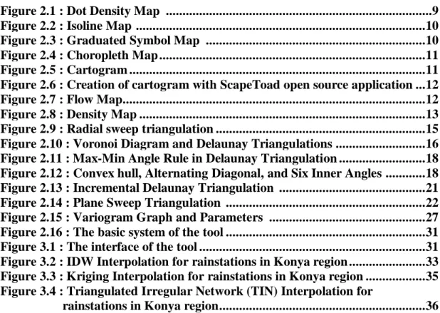
Delaunay triangulation is mentioned by B.Delaunay in 1934 (Yanalak, 2001). Voronoi diagram is the geometric match of Delaunay triangulation. Voronoi diagram is also referred to Dirichlet, Thiessen, or Wigner-Seithz diagram in the literature. Any point of the set of endpoints in the plane is called Voronoi Polygon instead of the geometry of the plane points that are closer to the other points in the cluster. The union of the Voronoi ridges of all the points in the cluster forms the Voronoi diagram of that rudder. This diagram is a definite structure used for the nearest point problems. The Voronoi polygon separates any point from its nearest neighbors. The edge of the polygon is composed of the center struts of the right parts connecting the point and neighboring points, and when each point is combined with its neighboring points, Delaunay triangulation is obtained (Yanalak, 2001).

Figure 2.10 shows the Voronoi diagram and Delaunay triangles of a point clusture.

Voronoi Diagram and Delaunay Triangulations (Tuncer, 2017) Figure 2.10 :

17

Some important features of delaunay triangles are listed below:  There is uniquness that independent from the starting point.

 The resulting triangles are the most likely equilateral triangles.The formation of very narrow-angle triangle, and thus establishing a linear relationship between the points which are distant from each other without relationship is prevented.

 There is no other point in the circum-circle of the triangles.

 The convex frame of the dataset is in triangle. The convex frame of a point clusture is the smallest polygon enclosing that cluster.

 Sample points are located in the triangle formed by the pair of points closest to each other in the cluster.

 The line segment that connects each point with the closest point to it constitutes a triangle edge.

Properties of Delaunay Triangulation

 Local Empty Circle Property;

No other reference point can be found in the circum-circle of a Delaunay triangle. It is the exception of this rule that 4 or more points are placed on the same circle. Algorithms should be taken into account in this particular case. A selection criterion is set for the algorithm for this contradiction. Circum-circle criterion is generally used in incremental algorithms. When the third point of each triangle is determined, it is checked whether there is another reference point in the circum-circle of these three points. If there is another point in the circum-circle, this point will be nominated to be the 3rd corner of the next triangle to be created. It is checked whether there is another point in the circumference circle of the candidate triangle. This process continues until no point remains within the circum-circle. There are two ways to check if there are other points in the circle. The first one is to compare the distances of the points to be checked to the center of the circle with the radius of the circle. The points with smaller distance from radius is located within the circle. The second way that can be used for control is to calculate the angles that see the known edge of the triangle. The angles that see the exact edge of the triangle at all points are calculated to control if these points are in the circum-circle. The angles at these points are compared with the angle at

18

which the third point of the triangle is considered to be formed. In this respect, points with larger angles are located within the circum-circle. Points with smaller angles are outside the circle. The presence of points with the same angle indicates that these points are on the same circle (Yanalak, 2001).

 Minimum Angle Property;

Interpolations for triangulation are defined as triangulations if the triangles are approximate to equilateral triangles. This property suggests careful selection of the diagonal of each convex rectangle formed in triangles (Yanalak, 2001). In Figure 2.11 PlPk which is the diagonal of tetrahedral obeys the max-min angle rule. PiPJ isn’t an appropriate diagonal. This property maximizes the minimum angle of the six internal angles according to the two possible triangulations of tetrahedral (Varshosaz et al., 2005).

Max-Min Angle Rule in Delaunay Triangulation (Varshosaz et al., 2005) Figure 2.11 :

Two triangles which share a common edge form a rectangle. The common edge is the diagonal of this tetrahedral. If this rectangle is convex (Figure 2.12), when the diagonal is replaced by an alternate diagonal it should not increase the value of the minimum of six angles of the two triangles forming the quadrangle. This rule should be provided for all convex rectangles.

Convex hull, Alternating Diagonal, and Six Inner Angles (Yanalak, 2001) Figure 2.12 :

19  Uniquness;

There is only a unique delaunay triangle that will consist of a set of points.  Boundary Property;

The external edges of the delaunay triangulation creates the convex hull of the point cloud (Varshosaz et al., 2005).

Evaluation of These Algorithms

There are some problems that should be solved for triangulation algorithms to respond to requests.

 Rapidity;

In addition to giving correct results, it is an indicator of effectiveness for an algorithm to give correct results in a short time. Operation duration depends on the algorithm running time of the software as well as the hardware used. For this reason, in order to observe the efficiency of the algorithm independently from the hardware, the increase of the working time is examined depending on the increase of the number of sample points. If it is considered that there are n number of reference points, it is expressed as an exponential function (logarithmic) between the number of reference points and the running time of the algorithms. Triangulation algorithms require several iterations of some calculations and queries. The calculation of the center of circum-circle and radius, the calculation of an inscribed angle that sees a chord, the questioning of whether a point is in a circle or whether there is another point in the circle can be given as an example. Such algorithms that require repeated dozens of times, accessing to the data or using the data as required are the two most important factors affecting the rapidity. The only way to access data quickly is only possible when the data is stored in an order. Achieving sequential data will save a lot of time. Even the sorting method to be used will greatly affect the speed of the algorithm. Partitioning the data set into boxes is another method used to speed up the algorithms. The data set is divided into equal intervals in the x and y directions. The boxes in which each reference point is located are determined by looking at the intervals at which the reference points are listed separately according to the x and y coordinates. Therefore, it is also determined which reference point is involved in

20

each box. Thanks to this box structure, the data field is divided into small pieces. It is not necessary to scan the entire data field using the corresponding reference points in the above mentioned account and inquiry processes. The entire data field does not need to be scanned because only the focal points in the corresponding boxes are used (Yanalak, 2001; Varshosaz et al., 2005).

 Storage;

The memory capacities of used computers aren’t infinite, even if they have increased. Memory shortages can arise when working with a large number of reference points. The memory problem occurs in different sizes depending on the characteristics of the programming language being used. Algorithms involving classifying of the data field provide an advantage in speed, but the information that should be stored increases. For this reason, information may need to be stored using special memory storage methods or different matrix structures. Memory storage methods which can be applied with the aim to save space in computer memory are storing matrix as a square format, storing the semi-matrix in linear form, storing the band matrix in rectangular form, storing band matrix in linear form, storing variable band matrix in linear form (Öztan, 1981; Yanalak, 2001). In the direct and incremental methods, the speed problem is more obvious, and the memory problem is less than the other methods. A good triangulation software should solve the problem of speed and storage adequately (Yanalak, 2001).

 Limitation of Data Field;

The data field to be triangulated must be defined with a boundary in order to cut off calculations in one place. Otherwise, the algorithms may go into an infinite loop, where they can not determine where to continue the neighboring point search, where to cut the operation. It may also be necessary to limit the data field in terms of the triangulation’s accuracy. In particular, unnecessary and misleading triangles are formed towards the ends of the zigzag land. In order not to get false information information through interpolation, the data field can be limited so that these triangles are out. The geometric shapes used until now to limit the data field are a triangle enclosing all of the reference points, a rectangle bounded by the smallest and largest x and y coordinates, or a selected polygon (Yanalak, 2001; Auerbach and Schaeben, 1990; Watson and Philip, 1984). The most widely used geometrical figure in

21

algorithms is polygon. In some algorithms, a polygon is defined as the initial data. While the algorithm is running, it accepts this polygon as the boundary. In many algorithms, this polygon is not initially given as data. The algorithm produces this polygon itself. This special polygon, which is defined as the natural boundary of the data field, is called the “convex hull” (Yanalak, 2001).

 Accuracy and precision;

Triangulation algorithms must be reliable and precise since a reliable surface is needed.

 Stablity;

An algorithm should keep its stability in different performances.

Triangulation algorithms can be divided into five general groups according to their solution methods.

a. Incremental Algorithms

Incremental methods perform triangulation by starting from a fulcrum within or near the data field and stepping through the other points into the network. Triangulation is defined within developing wave structure (Mustafa Yanalak, 2001).

Incremental Delaunay Triangulation (Varshosaz et al., 2005) Figure 2.13 :

b. Step by Step Algorithm

Triangulation starts from the edges forming the Convex Hull. The smallest edge in the convex hull is selected as the first edge. The third point, which forms the delaunay triangle, is found. Triangulation is controlled by a circle passing through these three points. If there are more than 3 points in the circle, the size of the circle must be changed. The points near the bisector of the basic line are selected (Varshosaz et al., 2005).

22 c. Filliping Algorithm

First, an artificial triangulation is created by using incremental triangulation algorithm. It is then optimized in accordance with the Delaunay triangles (Varshosaz et al., 2005).

d. Plane Sweep Algorithm

This method, which is one of the gradual of Delaunay triangulation methods. In this method all points are scanned with a line. This algorithm was first used by Fortune in 1987 (Varshosaz et al., 2005).

Plane Sweep Triangulation (Varshosaz et al., 2005) Figure 2.14 :

e. Divide and Conquer Algorithm

Divide-and-conquer methods are methods that divide the data field sequentially into sub-regions until the final triangulation occurs. The approach used to divide the data field is the basis of the algorithm. The triangular parts are then combined (Varshosaz et al., 2005).

2.2.1.3 Natural Neighbours Method

The natural neighbours method was developed by Sibson in 1981 with the principle of determining the value of a set of known points closest to the calculated points. In this method, new surface values are calculated by assigning a weight to each point in the known nearest point set relative to the area of the point (Öztan, 1981; Doğru et al., 2011). This interpolation technique, working on a weighted average, is very similar to the IDW interpolation technique. When searching for points to be interpolated, we use the distance-based weights at the sample points. It is an extremely easy technique which can distinguish and classify the sample data at irregular density, uses digital interpolation tools suitable for the general purposes of

23

interpolation logic and TIN functions together with an algorithm and does not require any special defined parameters. In this technique, first a triangulation is made with Delaunay triangulation that each sampling point is a triangular corner point. Then, convex areas are defined as the minimum number of triangular edges for each point. The weight of each neighboring point is assigned to these areas as determined by “Thiessen / Voronoi Technique”. In other words, Natural Neighborhood Interpolation Technique is a method based on “Thiessen Polygon Network”. Thiessen polygon network can be constructed on the delaunay triangulation obtained from the sampling points. There is a single thiessen polygon for each sampling point in the Thiessen polygon network (Arslanoğlu and Özçelik, 2005)

The weights are given below for i=1, 2,N and each neighbour’s area is (Webster and Oliver, 2001) (Equation 2.3)

∑ (2.3)

2.2.1.4 Inverse Distance Weighting Method

In IDW method, unknown surface data are calculated by using weighted point data. The weight defined for the points in the IDW is defined as a function of the distance between points (Childs, 2004). Within this scope, the effect of the function decreases as the distance increases (Doğru et al., 2011). The IDW interpolation technique is often the preferred method of interpreting grids from sample point data. The IDW interpolation technique is based on the principle that adjacent points on the surface to be interpolated have more weight than distant points. This technique interpolates a surface according to the weighted average of the sample points, which reduces weight as it moves away from the point to be interpolated. Although there are several IDW methods, the most known is "Shaperd's Method" (Arslanoğlu and Özçelik, 2005). "Shaperd's equality" is as follows, with the number of scattered points on the surface n, the function defining the sample points, and the weights . (Equation 2.4-2.5)

( ) ∑ (2.4)

24

p is known as the "power parameter" and usually refers to a positive real number taken as two. Besides defines the three-dimensional spatial distance between the sampling points and the point to be interpolated (Arslanoğlu and Özçelik, 2005) (Equation 2.6)

√( ) ( ) ( ) (2.6)

2.2.1.5 Regression Models

The existence of an interdependent relationship between some variables can be determined from the measurements and calculations made. An example of this relation is between the water level change at the upstream side of a dam (the water's rising and falling depending on season) and the deformation (horizontal and vertical displacements) occurring in the dam body, and the increase in landslide numbers depending on the amount of rainfall. The determination of the existence of this relationship and the power of the relationship is important for making predictions about the future. Regression analysis is an analysis method used to determine the relationship between two or more variables. If a single variable is used, it is called univariate regression. Otherwise if multiple variables are used, it is called multivariable regression called analysis. Regression analysis can determine the existence of the relationship between variables, and if there is a relation, it can determine the power of it. The regression expresses the functional form of the linear relationship between two or more variables (Bayrak, 2010). If the regression model will be set with a secondary variable, this variable is also called such as explanatory variables, auxiliary variables or ancillary variables. The information about this variable is called secondary information. The relationship between variables is determined with Akaike information criteria (AIC) or Bayesian information criteria (BIC) (Li and Heap, 2008).

2.2.1.6 Trend Surface Analysis

The tendency of observation values obtained for a time dependent variable to increase or decrease over a long period of time is called "trend". Trend tests are divided into parametric tests and nonparametric tests. Data with independent and normal distributions are used in parametric test, on the other hand only individual data are used in non-parametric tests which don’t have to be normal distribution.

25 Parametric tests;

• t test

• Simple linear regression model Nonparametric tests;

• Mann-Kendall test • Spearman's Rho test • Sen’s T test

Trend analysis gives information about the trend of data over time. The changes that occur between months, years and seasons can be made or comparisons may be made about and interpretation in the future (Kayıkçı and Beşel).

2.2.1.7 Splines and Local Trend Surfaces

Another group of approximation techniques, splines, are a special kind of joint polynomial and are preferred for simple polynomial interpolation. Spline function assumes that there is an error in the data therefore also needs to be a local correction (Aktaş and Yılmaz, 2012). The spline interpolation method creates an elastic surface, as if a rubber surface were stretched along known points instead of taking the average of the values as the IDW did. This stretching effect is useful if the estimated values are lower from the minimum values within the sample or higher the maximum values. In this way, the spline interpolation method is useful for estimating low and high values which aren’t added sample data (Başçiftçi et al., 2013).

There are a few spline methods such as B-Spline, Multi-Layer B-Spline, Cubic Spline, Thin Plate Spline (Aktaş and Yılmaz, 2012).

Local trend surfaces (LTS) fit into a polynomial surface for each projected point using nearby examples. There are two approaches in LTS. One is a local polynomial regression fitting that is detailed by Cleveland et al. (Cleveland and Devlin, 1988). The second is a bilinear or bicubic spline developed to apply two variant interpolations on a grid for irregularly spaced point data. This method is also known as Akima's interpolator (AK). Neither approach can choose straightness (Li and Heap, 2008).

26 2.2.1.8 Other Methods

Classification, Regression Tree, Fourier Series, Lapse Rate are used for spatial interpolation purposes (Li and Heap, 2008).

2.2.2 Geostatistical Interpolators

Geostatistics is an applied field of statistics and was first used to solve the problems encountered in earth sciences. By using geostatistical methods, unbiased and minimum variance estimates can be made by considering the positions of the points where the observations are made and the correlation between the observations. In geostatistical studies, an experimental variogram structure is determined from observation data and a theoretical model is created for this structure. Variogram is a function that characterizes the dependency between variables in different points in space. Variogram analysis is used to specify the degree of positional dependency of the feature being examined, that is the positional dependency between the measured points. On the other hand, kriging analysis is widely used in estimating the characteristics of points or areas that are not measured. For geostatistical analysis, firstly normal distribution test should be applied to the data. When non-normalized data are used, errors resulting from estimation will be higher. The histogram shows how often the observation values are distributed corresponding to certain intervals. Trend analysis provides a three-dimensional view of the data. Measured value at each measurement point indicated in the horizontal plane (N) is displayed as the third dimension. In the trend analysis, the reflections of the measurement values at the points are shown. These values can be defined by an appropriate polynomial. At the same time the indication on the graph of the trend in two directions is carried out. Normal QQplot is used to plot the standard normal distribution deviations of the observations on the graph. The variance of the difference between the values of the spatial variables in geostatistics is expressed by the variogram function. The variogram function is expressed as the variance of the difference between two positional variables at s distance from each other (Yaprak and Arslan, 2008).

The rules to be considered when calculating the semi-variogram are listed below. There must be enough sample pairs for the distance between the samples to be used in the calculations.

27

Since there will not be enough sample pairs, the variance diagram should not be calculated for more than half of the longest edge of the land.

In cases with irregular sampling the smallest sample interval must take as initial calculations (Yaprak and Arslan, 2008).

Variogram Graph and Parameters [22] Figure 2.15 :

Theoretically, when s = 0, the value of the variogram is equal to zero ( ) . The

distance value that can be determined from the distance dependent change is the distance between the two closest samples (Figure 2.15). In practice, the change of the difference between the values can not be determined at a smaller distance than this distance, which leads to a discontinuity in the origin of the variogram. One reason for discontinuity is the sampling and analysis mistakes. In the variogram, this situation manifests itself as a “nugget effect”. This value is also called the uncontrolled effects of variance. It does not affect the estimation value. It just causes changes in the kriging variance.

The cross validation method is used as a criterion in determining whether the theoretical semivariogram parameters can represent the field of study. Cross validation analysis is a method that compares the estimated values with the actual values by estimating the values at the measuring points included in the kriging method (Yaprak and Arslan, 2008).

Kriging, one of the powerful methods of calculation of surfaces, has been developed with the assumption that it includes a spatial relationship that can be used to describe the distance between known value points or the changes in the direction of the plane. Kriging interpolation method estimates the optimum value of the interpolation point by using data from other data received from the closest point. This is the prediction

28

technique of spatial changes in points made optimally using unsampled semi-variogram structural features (Doğru et al., 2011). The most important feature that distinguishes the Kriging method from other interpolation methods is that a variance value can be calculated for each estimated point or area. This is a measure of the degree of confidence of the predicted value. The Kriging technique is a technique that allows for calculation of the standard deviation of estimates with minimum variance, as well as more unbiased results than other estimation techniques. Semivariogram and covariance allow the assessment of the positional relationship between the measurement points. Measurements close to each other give close values to each other. Semiquarogram and covariance determine the level of this relationship (Yaprak and Arslan, 2008).

The Kriging method involves two different applications, ordinary and universal kriging, according to the function used (Doğru et al., 2011). The Kriging method is detailed in section 3.2.2.

29

A VISUAL ISARITHMIC MAPPING TOOL 3.

Today, many commercial Geographic Information System (GIS) software is used in the production of interpolation maps. However, this situation causes users to pay a large amount of money or use counterfeit programs. Although there are open source software that can create interpolation maps, users are faced with the situation of setting up a program to create an interpolation map. In addition, program information is also required. However, with the web-based mapping method we recommend, users will be able to evaluate and analyze information based on location on the Internet, regardless of where the world is located, without having to know or use the program. Because it is an open source tool and can be accessed over the Internet, it will be open to others.

Material and Method 3.1

There are three main languages that need to be known to produce web-based maps which are HTML, Javascript and CSS.

Hyper Text Markup Language (HTML) is a markup language that enables web pages and other information to be displayed on web browsers. Html is a coding language that is officially recommended by the World Wide Web Concorcium (W3C) and is also accepted by most popular web browsers. The formatting language tells client computers how to display fonts, images, and other elements on web pages. HTML codes are rendered into page content through Html elements (<h1>, <html>, <img>, etc.) placed between the tags "<" and ">". The tags specified are usually used in pairs. The first one specifies the beginning of "<html>" and the second one is written in "</ html>" format and is used for termination. Thus, web browsers read the HTML elements between the start and end tags and read the web page styles that will be displayed in web browsers (World Wide Web Consortium, 2018; Sarı, 2014). JavaScript is a coding language that makes static websites dynamic, individual and interactive. It is one of the common coding languages used to provide complex features to web pages. JavaScript has received many names and naming methods from the Java language, though both languages are structurally different from each other and independent software languages. Operating principles of the JavaScript scripting language written Influenced by C language is taken from the Self and

30

Scheme programming language. Since JavaScript language is not a compiled language, there is no programming or coding environment required when writing JavaScript code. For this reason, while writing codes, text editors can be used in the simplest sense. Thus, JavaScript codes can be generated independently of the software (World Wide Web Consortium, 2018; Sarı, 2014).

Leaflet is an open source web map display library the modular structure, the extremely small library size, and therefore the performance load times are remarkable. Because it is a new library, it uses almost all the new web technologies, so it has an important effect on the web as well as on the web. It is completely free to use (Dinçer et al., 2013). The Leaflet is used in this thesis which is an open source JavaScript library for interactive maps. Leaflet uses OpenStreetMap (OSM) as a basemap. OpenStreetMap is a world map created by volunteered people, free to use and under open license. In web based map applications, Web Merkator projection system is used. Initially it is started to use in 2005 by Google, the Web Mercator projection has become a standard for nearly all popular web mapping services, such as Google Maps, Bing Maps, OpenStreetMap, MapQuest, ESRI, and Mapbox. Web Mercator, is a modified version of the Mercator projection. Although it is derived from Mercator projection, this projection isn’t conformal(Bildirici And Kırtıloğlu, 2016).

Style sheets (CSS) facilitate the development of pages of different styles in addition to HTML (Aslan, 2007).

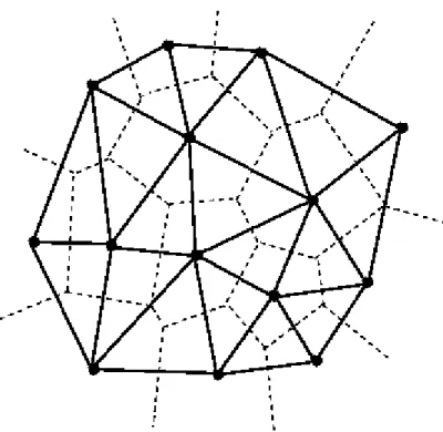
In Figure 2.16 the basic system of our tool can be seen. Firstly users upload their own data after that the algorithm calculates the bounds of uploaded data. And then users enter cell size. Finally the isarithmic map is produced for chosen interpolation method.

31

The basic system of the tool Figure 2.16 :

Thematic Mapping 3.2

Users will be able to make their own interpolations by uploading their own data (gpx, kml, geojson and csv file formats) over the internet, no matter where they are. These files are converted to geojson and processed. In Figure 3.1, users will upload their data from the left side button. After then, they will calculate the bounds of uploaded data from the right side navigation bar. Finally they will produce their own isarithmic map.

32 3.2.1 IDW Interpolation

The idw method has been applied on the sample dataset for the rain stations in Konya region. The result map was colored as a choropleth map using leaflet.js choropleth plugin. Turf.js’s IDW plugin was integrated to geoprocess the geojson data. Various JavaScript libraries should be integrated in the body of the code document. Leaflet.js, turf.js and choropleth.js have been integrated for map canvas, interpolation and legend. Turf.js uses the basis function of the IDW. Firstly, the algorithm creates grid which surroundes the boundary box of the control points. The cell width is entered by the user. The algorithm produces seven thematic classes. These are also colored according to the choropleth plugin and the legend is automatically drawn. 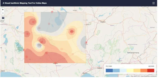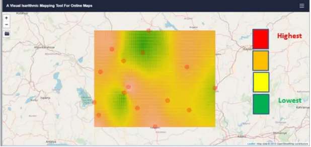IDW is based on the following basic equation (Equation 3.1, 3.2).

̂

̂

In the equations given above ̂ is the value to be estimated and is the known value of the control point. In the second equation given above p is the power of the interpolation. p value in this study is taken as 1. Rain station measurement data is interpolated according to the “intensity” value in the geojson file entered and seven thematic classes are created. Limit values are calculated by the algorithm as 23.2 mm and 42.9 mm. The blue color shows lower values while the red color shows higher values. If small cell width is selected, the result map looks like raster, but the process time is getting longer (Figure 3.2).

33

Figure 3.2 : IDW Interpolation for rainstations in Konya region 3.2.2 Kriging Interpolation

Kriging interpolation is a technique in which the unbiased estimation of the positional changes at the unsampled points is made optimally using semivariogram structural features. The most important feature that differentiates the Kriging method from other interpolation methods is that a variance value can be calculated for each estimated point or area, which is a measure of the confidence level of the estimated value. The basic equation used in Kriging is given below.

̂ ∑

Here; n is the number of points forming model, ̂ is the value to be estimated and is the known value of the control point, is the weight value of values. The calculation of the weights to be given to the values of vi is determined as the average of the estimation errors is zero and the variance is minimum. Expected value should be . To achieve this, ∑ equality should be provided. For the minimum variance, [ ] . It is desirable that the weight totals are equal to 1 so that the interpolation is unbiased. In this case there are n unknown and n + 1 equations. The Lagrange multiplier is added for the solution to be unbiased. Thus, the number of equations is equal to the unknown number. Weights are obtained from the following equation using the variogram functions.

34

Here P is the weight matrix, is the semivariogram matrix between base points, is the the semi-variogram matrix between the base points and the predicted point. The predicted values for each point are calculated after determining the weights. The kriging variance of the interpolation point is found by the following equation.

(3.5)

Here is the transposed matrix of the weight matrix, is the kriging variance. The kriging technique is a technique that allows for calculation of standard deviation of the estimated value with minimum variance as well as more unbiased results than other estimation techniques (Yaprak and Arslan, 2008).

Kriging.js with MIT licence is used in this study. Kriging.js uses ordinary krging algorithm. In the Ordinary Kriging method, the solution is based on the assumption that the variables are stationary and the average is constant. In practice, it is often the case that regional variables are not stationary and show a trend. The fact that the data show a trend and the solution of the Kriging system by joining the account in this trend is called Universal Kriging (Cevat and YİĞİT, 2004). In this study, variogram model can be specified as gaussian, exponential or spherical. Exponential model has been chosen (Figure 3.3).

<script src="kriging.js" type="text/javascript"></script> <script type="text/javascript">

var t = [ /* Target variable */ ]; var x = [ /* X-axis coordinates */ ]; var y = [ /* Y-axis coordinates */ ]; var model = "exponential";

var sigma2 = 0, alpha = 100;

var variogram = kriging.train(t, x, y, model, sigma2, alpha);

</script>

(sigma2) and α (alpha) variables correspond to the variance parameters and the prior of the variogram model.

35

Figure 3.3 : Kriging Interpolation for rainstations in Konya region 3.2.3 TIN Interpolation

Turf.js’s TIN package has been used for this algorithm. Here, colorRamp function has been used for the color range. The corresponding code is given below.

var tin = turf.tin(dots, 'intensity')

for (var i = 0; i < tin.features.length; i++) { var properties = tin.features[i].properties;

properties.average =

(properties.a+properties.b+properties.c)/3;

if (properties.average > maxAvg) maxAvg =

properties.average; }

colorRamp = chroma.scale('YlGnBu');

L.geoJson(tin, {onEachFeature: onEachTri, style:

tinStyle}).addTo(map);

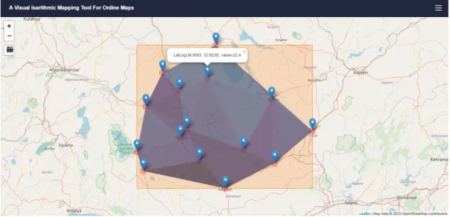
The TIN (Triangulated Irregular Network) consists of a set of non-overlapping triangles that vary in size and proportions. Points, lines, and polygons are used as inputs to form the TIN. When the TIN is created, the input points become the corners of the triangles. The corners are connected by lines that will form the edges of the triangles. As a result, a continuous triangle surface consisting of the edges is obtained. The point data without Z value can be used to define the boundary lines of the area while generating TIN. In the TIN data, there are height, slope and information value of the surface (Başçiftçi et al., 2013) (Figure 3.4).

36

Figure 3.4 : Triangulated Irregular Network (TIN) Interpolation for rainstations in Konya region