A GIS BASED NEW NAVIGATION APPROACH FOR REDUCING EMERGENCY VEHICLE'S RESPONSE TIME
1Fatih SARI
1Selçuk University Çumra Vocational School Konya, TURKEY
(Geliş/Received: 07.09.2016; Kabul/Accepted in Revised Form: 04.01.2016)
ABSTRACT: Recently, for ensuring human life and safety, routing and intervening emergency vehicles
as soon as possible an important subject. Ambulance, firefighter, police and other emergency vehicles are the main object of the intervention. Reaching the emergency area as soon as possible is important for saving human life and preventing economic loss. Directing and routing emergency vehicles from the moment they receive an emergency call to the event location must be considered carefully. In this study, ensuring the shortest response time for the emergency vehicles, obstacles like speed bumps, traffic lights, parking status of the streets, railroad crossings and crossroads which reduce the speed of emergency vehicles and increasing the intervention time are detected. In order to determine the effect of obstacles, a new Segment Effect Value (SEV) formula is developed. Values are assigned to the street segments according to obstacles in particular streets. SEV formula makes possible to determine the routes that provides the shortest intervention time. Results are compared with the shortest route and the shortest time route.
Key Words: Emergency response time, Network analyst, Geographical information systems, Navigation systems
Acil Müdahale Araçlarının Müdahale Zamanını Azaltmak İçin Cbs Tabanlı Bir Navıgasyon Yaklaşım ÖZ: İnsan yaşamını ve güvenliğini sağlamak için acil durum araçlarının olabildiğince hızlı müdahalesi
önemli bir konu haline gelmiştir. Ambulans, itfaiye, polis ve diğer araçları acil durum müdahale araçlarının başında gelmektedir. Yaşam kayıplarının ve ekonomik kayıpların önüne geçmek için hızlı müdahale büyük önem taşımaktadır. İhbar alınmasından itibaren olay yerine gidene kadarki yönlendirme dikkatle yapılmalıdır. Müdahale zamanını kısaltmak için hız bariyerleri, trafik ışıkları, park etmiş araçlar, demiryolu geçitleri ve kavşaklar gibi hız kesici engellerin bilinmesi gerekmektedir. Bu engellerin etkisini ortaya koymak için Segment Etki Değeri (SED) isimli bir formül geliştirilmiştir ve bu formül ile her bir cadde segmentine değer atanmıştır. Böylece araçların bu engellerle karşılaşmayacakları en hızlı güzergah üzerinden gitmelerinin sağlanması amaçlanmıştır. En kısa yol ve en hızlı yol arasındaki farklar paylaşılmıştır.
Anahtar Kelimeler: Acil müdahale zamanı, Ağ analizi, Coğrafi bilgi sistemleri, Navigasyon sistemleri INTRODUCTION
The importance of intervention methods are increasing in health, crime, fire and natural disasters (Paraskevi et al., 2010; Konstantinos et al., 2000, Zhang et al., 2016; Lam et al., 2015). Responding to emergency call needs to be managed effectively using decision support systems to save human life and
provide public security (Bandyopadhyay and Singh, 2016). Generating decision support systems provide the right decisions in emergency situations and manage the reasons and solutions of the emergency status (Yoon et al., 2008; Mincardi et al., 2007; Aktas and Swalehe, 2016).
Technological developments have led to new techniques in vehicle routing processes. Emergency vehicles use navigation devices to find the shortest routes. These devices lead vehicles to a marked destination point and determine the shortest route. One the other hand, when the working principle is considered, it can be observed that the navigation considers only directions, highways, primary and local roads. This method principle provides only the shortest route information to the emergency vehicles. In addition to this, emergency stations direct vehicles using vehicle tracking systems, but neither drivers nor emergency station workers know the situation on the street itself. Besides, sometimes driver experiences maybe more reliable then the navigation. Additionally, there are various obstacles which reduce vehicle speed. Speed bumps, traffic lights, parking status, railroad crossings and crossroads are the main obstacles for emergency vehicles. When emergency vehicles encounter one of these obstacles, vehicles are forced to slow down or even recalculate or change their route.
In the literature, there are some predicted values about response time of the vehicles. Mohd et al, (2008), provide response times for some countries as shown in Table 1.
Table 1. Ambulance response times 1
Country ART(Minutes) United Kingdom Australia Ankara, Turkey Singapore 7-14 7-11 9 15 ED of HUSM 15.20
City of New York City of Chicago
11.40 11.30
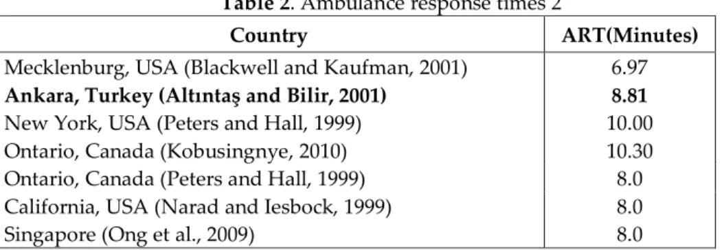
Ateş et al, (2011), in their work for determining most appropriate locations for ambulance stations, give also other response times as can be seen in the Table 2.
Table 2. Ambulance response times 2
Country ART(Minutes)
Mecklenburg, USA (Blackwell and Kaufman, 2001)
Ankara, Turkey (Altıntaş and Bilir, 2001)
New York, USA (Peters and Hall, 1999) Ontario, Canada (Kobusingnye, 2010)
6.97
8.81
10.00 10.30
Ontario, Canada (Peters and Hall, 1999) 8.0
California, USA (Narad and Iesbock, 1999) Singapore (Ong et al., 2009)
8.0 8.0
As is shown, there is quite a short time to decide, travel and intervene. All the parameters and obstacles must then be known by the drivers and emergency staff to provide the shortest response time.
In the literature, there are a lot of investigations concerning decision support, emergency response and vehicle routing problems (VRP), which developed new methods, new algorithms and emergency response simulations. Many of these are interested in the mathematical algorithm of the methods which are used for vehicle routing. Some of them focused on the simulations that represent the emergency response.
Huang et al., (2012), created a framework for the purpose of response to traffic accidents on highways. Haghani et al., (2003), proposed an optimization model for vehicle routing and dispatching in real time. Liu and Hall, (2002), developed a software to analyze accidents and dispatch ambulances to the accident area. Ozbay and Bartın, (2003), developed a simulation for the analysis of traffic accidents in different situations. Campell et al., (2008), studied routes after disasters using two different methods. Stefan and Walter, (2014), proposed a warehouse location routing problem (WLRP) method and a new formula. Kerstin et al., (2011), studied on high speed ambulances for time savings. Ho and Casey, (1998), Ho and Lindquist (2001), studied on the sirens and lights of ambulances and their time savings in urban areas and in rural areas. Brown et al., (2000), investigated the effects of sirens and lighting of ambulances response times.
In order to determine the shortest route, Ahuja et al., (2002), developed a model to find the shortest travel time. Ziliaskopoulos and Mahmassani, (1993), worked on the shortest route for highway vehicles.
In the literature, it is seen that when determining routes, obstacles were not considered. Generally, the shortest way may not correspond to the shortest time because of the speed factor on route. In this work, obstacles are considered to find the shortest time in addition to the shortest way.
MATERIAL AND METHOD
The purpose of this study is to develop a model providing the shortest response time for emergency vehicles involving street structure and the environment. The model is based on six steps. These are namely; determining of obstacles, choosing the study area, digitizing, calculating the effect coefficient of obstacles, generating Segment Effect Value (SEV) formula and finally determining and comparing the routes.
Determination of the Obstacles
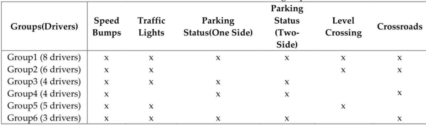
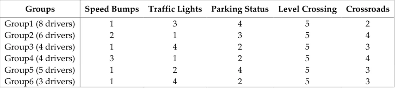
In the first step a discussion was made to detect the obstacles faced by 30 drivers of some emergency vehicles, chosen from 6 different emergency stations. The two questions asked to the drivers were the type obstacles reducing the speeds of vehicles and the importance of specified obstacle. As is shown in Table 3 and 4, the drivers declared 5 types of obstacles namely, speed bumps, traffic lights, parking status, level crossings and crossroads. They claimed that especially speed bumps and traffic lights reduce vehicle speeds considerably. Although the emergency vehicles have transition superiority at traffic lights, the other vehicles waiting usually prevent using this superiority. Parking status and level crossings are less effective obstacles since they depend on width of the street and the frequency of closed level crossings. Particularly in narrow streets, parking status strongly affects the vehicle speed.
Table 3. Obstacle distribution to groups
Groups(Drivers) Speed Bumps Traffic Lights Parking Status(One Side) Parking Status (Two-Side) Level Crossing Crossroads Group1 (8 drivers) Group2 (6 drivers) Group3 (4 drivers) Group4 (4 drivers) Group5 (5 drivers) x x x x x x x x x x x x x x x x x x x x x Group6 (3 drivers) x x x x x
Deciding the Study Area
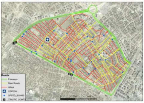
Study area was chosen a region in the city of Konya, Turkey, which has a population of 1.250.000 in the city centre. The population of the region is 4250 which is approximately a responsibility area of one ambulance. Its properties reflect the aim of the study and have freeways, main roads and alleys. There are narrow streets with parking on two sides and the surrounding area is covered by three lane freeways. There exist speed bumps, traffic lights and crossroads in the study area. It has totally 498 street segments with intensively occupied residence buildings. The study area is shown in Figure 1.
Table 4. Obstacle importance
Groups Speed Bumps Traffic Lights Parking Status Level Crossing Crossroads
Group1 (8 drivers) Group2 (6 drivers) Group3 (4 drivers) Group4 (4 drivers) 1 2 1 3 3 1 4 1 4 3 2 2 5 5 5 5 2 4 3 4 Group5 (5 drivers) 1 2 4 5 3 Group6 (3 drivers) 1 4 2 5 3
Figure 1. Study area Digitizing
In this process, all the street segments are digitized by ArcGIS software with using aerial imagery to use the network analyst extension. For the purpose of routing, street names are stored in the database with segment geographic information. After the digitization process, speed bumps, parking status and traffic lights are positioned using Google Earth Street view extension. As can be seen in Figure 2, speed bumps, traffic lights and parking status of segments are defined clearly by using street view. Then the obstacles are integrated with street map by using ArcGIS software and the coordinates are linked with the street segments as attribute data. The parking status of each segment is investigated as one-sided or two sided.
Figure 2. Google Earth street view for obstacle detection
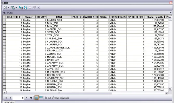
In Figure 3, the attribute table of the segments are given. Name column represents the names of the segments to be able to use street names in route navigation process. Parking status column includes a code list that explain one sided parking (1), two sided parking (2) and no parking (3). Similar to parking status, speed bumps are converted to 1 (segment include speed bumps) and 2 (no speed bump) codes. The width of the street is related to parking status and the maximum limit of the emergency vehichle. The codes then will be used in Segment Effect Value to calculate the delay times for each segment.
Figure 3. Digitized study area with obstacles and parking status Calculating the Effect Coefficient of the Obstacles
Obstacles affect vehicle speeds for different time periods. In order to determine the time delay on vehicles, information on 54 routes of 10 emergency vehicles were obtained from the vehicle tracking systems. The route information includes the speed of the vehicle at any time, acceleration-deceleration information and total response. The streets in the 54 routes were examined considering the obstacles and motions of the vehicles in order to find the delay time of the 10 different vehicles.
The calculated effects and delay times are shown in Table 5 for speed bumps, parking status (one-side), parking status (two-(one-side), traffic lights, level crossings and crossroads. For each obstacle two time
values have determined to find the delay time. The first values are the travel times with 50 km/h fixed speed without any obstacles. The second values are the travel times of the vehicles with obstacles. The difference between these two values gives the delay time. Finally, the average delay time of 10 different vehicles assigned as the delay time of the stated obstacles. Delay times of the obstacles are shown in the Table 5.
Table 5. Delay times
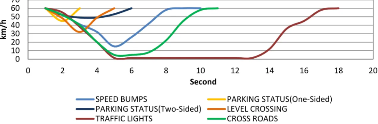
In Figure 4, acceleration graphics of the vehicles are shown for each obstacle. The graphics are drawn by using the average of the values obtained from 10 different vehicles values.
0 10 20 30 40 50 60 70 0 2 4 6 8 10 12 14 16 18 20 km /h Second
SPEED BUMPS PARKING STATUS(One-Sided)
PARKING STATUS(Two-Sided) LEVEL CROSSING
TRAFFIC LIGHTS CROSS ROADS
Figure 4. Acceleration graphics Generating Segment Effect Value (SEV) Formula
Each road segment may contain one or more obstacles. For example speed bumps, two side parking and at the end of the street traffic lights may exist. Each segment should be examined with the obstacles it has. For finding the total effect of the obstacles on vehicle speeds, total delay time value should be calculated. To do this, Segment Effect Value formula is developed to calculate a delay time for each segment. Finally, these values will be used in determining the shortest response time routes.
The Segment Effect Value Formula is,
(1)
Where n is the count of objects, Si, POi ,PTi ,Ti, Li are the delay times in second and SLi is the road segment length in meter. The coefficients are representing;
Si: Speed Bumps (sec);
Poi: One-Side parked streets (sec), Pti: Two-Side parked street (sec), Ti: Traffic Lights (sec),
Obstacles Delay time(Sec)
Speed Bumps 7.83
Parking Status(One-Sided) 2.05 Parking Status (Two-Sided) 6.22
Traffic Lights 18.02
Level Crossing 3.24
In SEV formula, parking status coefficients are multiplied with the segment length and divided by 100 meter. The reason for this is parking status affects the vehicle continuously until the end of the segment. For example, if one vehicle is drawn at 50 km/h speed, in a road with one sided parking status the actual vehicle speed is 47 km/h. This status therefore, is affecting the vehicle speed depending on the segment length. The other obstacles are also affecting the vehicle speed at the point of obstacles the vehicles pass through the obstacles. Then the coefficients should be multiplied by the number of concerned obstacles. Multiplying the obstacle number by the coefficient gives the total effect. For example, in one segment if there is no speed bump, “n” value will be equal to zero and there will be no speed bump effect.
Delay times are determined by using the SEV formula for each 498 segments. Some of these values are shown in Table 6. SEV determining includes total delay time considering the obstacles that segments have as a sum of every obstacle delay time which are given in Table 5. Si, Poi, PTi, Ti and Li values represent the delay times for each obstacle and nSi, nPOi, nPTi, nTi, and nLi values represent the count of obstacle in each segment. As shown, segments number 17, 56 and 223 provide the shortest response times for vehicles with minimum delay times. These segments are seen to be freeways without traffic lights.
Table 6. SEV determining Segment
Number
Segment
Length nSi Si nPOi POi nPTi PTi nTi Ti nLi Li
Delay Time(sec) 1 375.85 0 7.83 1 2.05 0 6.22 0 18.02 0 3.24 7.83 19 519.96 1 7.83 0 2.05 1 6.22 0 18.02 0 3.24 18.49 56 331.73 0 7.83 0 2.05 0 6.22 0 18.02 0 3.24 0.00 < … … … … 182 223 257 311 424 107.25 359.93 113.06 30.47 356.24 1 1 1 1 0 7.83 7.83 7.83 7.83 7.83 1 0 1 0 0 2.05 2.05 2.05 2.05 2.05 0 0 0 1 1 6.22 6.22 6.22 6.22 6.22 0 0 0 0 1 18.02 18.02 18.02 18.02 18.02 0 0 0 0 0 3.24 3.24 3.24 3.24 3.24 10.02 7.83 10.14 8.45 29.46 Another example is the segments 19 and 311. Although these segments have the same obstacles, their effect delay times are different since their lengths are different. In 311, the vehicle will return or pass to another segment after a speed bump under its normal speed. But in segment 19, after passing a speed bump for 520 meters the vehicle reaches its normal speed. So, the SEV formula is considers the segment length and calculates the delay times.
Determining and Comparing the Routes
As a result, routes in status are calculated by ArcGIS Network Analyst Tool, the shortest path and the shortest response time. There are two network datasets for each situation and some properties are the same for both network datasets. These are lengths and travel time properties. Travel times are the time which vehicles need to pass through the segment and total route. Travel times calculated for 40, 50 and 60km/h speeds. This value changes with which segment route is followed. With these different calculations, the travel time will be estimated more accurately.
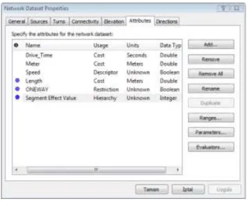
For calculating the shortest response time routes, a new facility is added to the network dataset. This is a hierarchy property which will decide the shortest response time route. The hierarchy property is shown in network dataset properties window in Figure 5.
Figure 5. Network dataset properties
.
In this network dataset, the entire segment’s effect values are stored in segment attribute table and by using hierarchy; a decision making process calculates the route comparing the effect values and choose the segments. The routes follow the segments having fewer obstacles. By hierarchy, 3 intervals are specified to make a preference between segments comparing the Segment effect values. These interval groups are given in Table 7. As shown, the first interval (0-5) represents the best segments for the shortest response time. The second interval (5-18) is for the normal segments. These segments will be used if there are no segments for which segment effect value is in the first interval. The third interval (18-50) has the worst segments that most reducing vehicle speeds considerably.
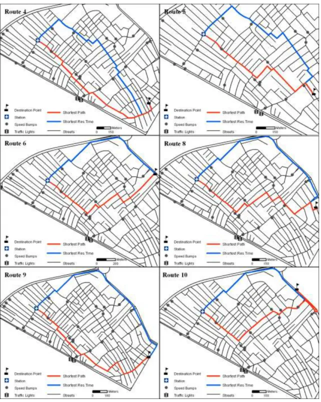
Finally, to see the results, all calculated values and the routes are compared by using both numerical and graphical methods. In Figure 6, the shortest route and the shortest response time routes are shown for the same origin and for 8 different destination points. The blue routes are the shortest response time routes and the red routes are the shortest distance routes.
Table 7. Hierarchy interval Group Interval(sec)
1 0.00-0.05
2 0.05-0.18
Figure 6. Routes and comparisons
One of the important obstacles which affect the vehicle speeds are crossroads. Crossroads may reduce vehicle speeds to zero and according to the type of vehicle it takes some time to reach to the normal speed. One important point is that, the crossroads can only be calculated after determining the routes, because we actually do not know where the route will go and how many crossroads the vehicle will encounter. Therefore, the crossroad factor is not considered in the SEV formula and it will be added to the total travel time of the shortest route or the shortest response time route. The final results are given in Table 8.
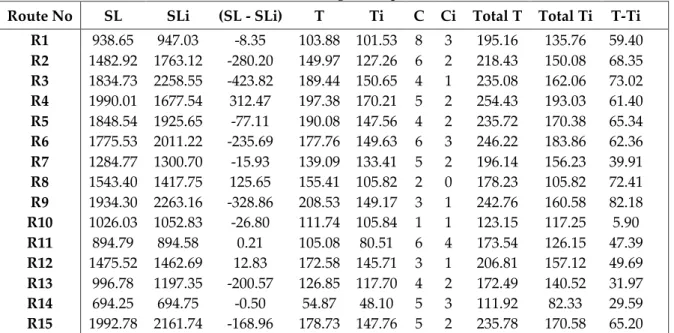
In Table 8, SL represents total length of the shortest way route, SLi total length of the SEV route, T is travel time of shortest way route, Ti travel time of SEV route, C is crossroad number of shortest way route, Ci crossroad number of SEV route, Total T is total travle time of shortest way route, Total Ti total travle time of SEV route and T-Ti is the benefit of travel times in second unit. .
As can be seen from Table 8, the travel time is calculated for each of the 15 routes. When the results are compared, it is shown that vehicles are gaining a minimum of 5.9 and a maximum of 82.18 seconds. In routes that follow freeways, the vehicles can go faster in the shortest response time routes. (Figure 6-a.b.e.g.h). On freeways there are only traffic lights, and therefore vehicles are going faster than in alleys. One advantage of the freeways is having less crossroads, so the vehicles can travel at a fixed speed.
Table 8. Time and length compare of two situation
Route No SL SLi (SL - SLi) T Ti C Ci Total T Total Ti T-Ti
R1 938.65 947.03 -8.35 103.88 101.53 8 3 195.16 135.76 59.40 R2 R3 R4 R5 R6 R7 R8 R9 R10 R11 R12 R13 R14 R15 1482.92 1834.73 1990.01 1848.54 1775.53 1284.77 1543.40 1934.30 1026.03 894.79 1475.52 996.78 694.25 1992.78 1763.12 2258.55 1677.54 1925.65 2011.22 1300.70 1417.75 2263.16 1052.83 894.58 1462.69 1197.35 694.75 2161.74 -280.20 -423.82 312.47 -77.11 -235.69 -15.93 125.65 -328.86 -26.80 0.21 12.83 -200.57 -0.50 -168.96 149.97 189.44 197.38 190.08 177.76 139.09 155.41 208.53 111.74 105.08 172.58 126.85 54.87 178.73 127.26 150.65 170.21 147.56 149.63 133.41 105.82 149.17 105.84 80.51 145.71 117.70 48.10 147.76 6 4 5 4 6 5 2 3 1 6 3 4 5 5 2 1 2 2 3 2 0 1 1 4 1 2 3 2 218.43 235.08 254.43 235.72 246.22 196.14 178.23 242.76 123.15 173.54 206.81 172.49 111.92 235.78 150.08 162.06 193.03 170.38 183.86 156.23 105.82 160.58 117.25 126.15 157.12 140.52 82.33 170.58 68.35 73.02 61.40 65.34 62.36 39.91 72.41 82.18 5.90 47.39 49.69 31.97 29.59 65.20 The most remarkable result of this study is that usually the shortest response time routes are longer than the shortest way routes. For instance, Route 3 in Table 8, the shortest response time route is 424 meter longer than the shortest route. If have a look to the response times, the shortest response time route results a gain of 73 seconds. This is a serious time to intervene to the emergency calls like fire and heart attack. The SEV formula may provide faster and earlier intervention for emergency calls. SL-SLi, T-Ti, Total T-Total Ti and nC-nCi comparisons are given in Figure 7.
50 100 150 200 250 R1 R2 R3 R4 R5 R6 R7 R8 R9 R10 R11 R12 R13 R14 R15 Se co n d Routes T Ti 0 2 4 6 8 10 R1 R2 R3 R4 R5 R6 R7 R8 R9 R10 R11 R12 R13 R14 R15 Se co n d Routes nC nCi
Figure 7. Routes and comparisons RESULT AND DISCUSSION
Traditional navigation systems determine routes with only limited parameters. These systems do not give actual travel times to the vehicles on shortest routes. In emergency calls, human life especially
depends on the travel times of the emergency vehicles. Considering the vehicle, sizes and emergency types, the travel times are being more important. By the Segment Effect Value formula, the shortest response time route can be calculated as well as the shortest route. Therefore, the formula provides the vehicles the most suitable routes allowing vehicles to gain a respectable time for intervention. At this point, data collection and defining routes should be investigated carefully. Especially closed or under construction roads, speed bumps and recent traffic status should be updated periodically. Nowadays, some municipalities have traffic monitoring and automatic vehicle counting systems to determine the traffic status of cities. Addition to this, Google Traffic service provides real time traffic data for main roads of the cities. This study can be integrated with one of these systems to determine real time navigation. Closed or roads that under construction data can be retrieved from the General Directorate of Highways provincial offices to determine real time shortest response time routes.
On the other hand, determining new fire and ambulance station locations can be investigated via SEV infrastructure. Thus, more realistic intervention times and related locations can be determined more accurately. New service areas, location-allocation and vehicle routing problems, which are related to network analysts, should be investigated for all emergency stations with environmental parameters such as population, topography of the streets and regions like industry, living and agriculture.
This study can be modified according to the types of emergency vehicles and for different conditions of the regions and countries. Especially for large vehicles, street width parameter can be added to the SEV Formula. The SEV Formula is designed allowing for adding new parameters.
REFERENCES
Ahuja, R., Orlin, K., James, B., Pallottino, S., Scutella, M. G., 2002, Dynamic Shortest Paths Minimizing
Travel Times and Costs, MIT Sloan Working Paper; No. 4390-02.
Aktas, S.G., Swalehe, M., 2016, “Dynamic Ambulance Deployment to Reduce Ambulance Response Times using Geographic Information Systems: A Case Study of Odunpazari District of Eskisehir Province, Turkey”, Procedia Environmental Sciences, Vol. 36, pp. 199 – 206.
Altınbaş, K. H., Bilir, N., 2001, Ambulance Times of Ankara Emergency Aid and Rescue Services Ambulance System”, European Journal of Emergency Medicine, Vol. 8, pp. 43-50.
Ateş, S., Coşkun, Z. M., Aydınoğlu, A. Ç., “Coğrafi Bilgi Sistemleri ile En Uygun Ambulans Yerlerinin Belirlenmesi”, 13. Türkiye Harita Bilimsel ve Teknik Kurultayı, Ankara, 18-22 Nisan 2011.
Bandyopadhyay, M., Singh, V., 2016, “Development of Agent Based Model For Predicting Emergency Response Time”, Perspectives in Science, Vol. 8, pp. 138—141.
Blackwell, T. H. Kaufman, J . S., 2001, “Response Time Effectiveness: Comparison of Response Time and Survival in an Urban Emergency Medical Services System”, Academic Emergency Management, Vol. 9, pp. 288-295.
Brown, L.H., Whitney, C.L., Hunt, R.C., Addario, M., Hogue, T., 2000, “Do Warning Lights and Sirens Reduce Ambulance Response Times?”, Prehospital Emergency Care, Vol. 4, pp. 70–74.
Campbell A, M., Vandenbussche D., Hermann W., 2008, “Routing for Relief Efforts”, Transportation
Science, Vol. 42, pp. 127–145.
Haghani, A., H. Hu., Q. Tian., “An Optimization Model for Real-Time Emergency Vehicle Dispatching and Routing”. In: the 82nd Annual Meeting of the Transportation Research Board, Washington, D.C., 12-16 January 2003.
Ho, J., Casey, B., 1998, “Time Saved with Use of Emergency Warning Lights and Sirens During Response to Requests for Emergency Medical Aid in Urban Environment”, Annals of Emergency Medicine,
Responding to Requests for Emergency Medical Aid in A Rural Environment”, Prehospital
Emergency Care, Vol. 5, pp. 159–162.
Huang, D., Chu, X., Mao Z., 2012, “A Simulation Framework for Emergency Response of Highway Traffic Accident”, Procedia Engineering, Vol. 29, pp. 1075 - 1080.
Kerstin P., Jan, P., Jörgen, J., Gun N., 2011, “Time Saved with High Speed Driving of Ambulances”,
Accident Analysis and Prevention, Vol. 43(3), pp. 818–822.
Kobusingye OC, Hyder AA, Bishai D, Joshipura M, Hicks ER, Mock C., 2010, Emergency Medical
Services,New York: John Wiley & Sons Ltd; 2010.p.167-. 169. 17.
Konstantinos G. Zografos., George M. Vasilakis., Ioanna M. Giannouli., 2000, “Methodological Framework for Developing Decision Support Systems (DSS) for Hazardous Materials Emergency Response Operations”, Journal of Hazardous Materials, Vol. 71 (1–3.7), pp. 503–521. Lam, S.S., Zhang, J., Zhang, Z. C., Oh, H. C., Overton, J., Ng, Y. Y., Ong, M. E., 2015, “Dynamic
Ambulance Reallocation for The Reduction of Ambulance Response Times Using System Status Management”, The American Journal of Emergency Medicine, Vol. 33, pp. 159-166.
Liu, H., Hall, R., 2002, W. INCISIM: User’s Manual. California Path Research Report; UCB-ITS-PWP-2000-15. Minciardi, R., Sacile, R., Trasforini, E., 2007, “A Decision Support System for Resource Intervention in Real-Time Emergency Management”, International Journal of Emergency Management, Vol. 4 (1), pp. 59-71.
Mohd, S., Mohd, I., Syed, M., 2008, “Ambulance Response Time and Emergency Medical Dispatcher Program: A study in Kelantan, MALAYSIA”, Southeast Asian Journal of Tropical Medicine and
Public, Vol 39 (6).
Narad, R. A., Iesbock, K. R., 1999, “Regulation of Ambulance Response Time in California”, Prehospital
Emergency Care, Vol. 3, pp. 131-135.
Ong M, E., Ng FS., Overton J., Yap S., Andresen D., Yong DK., Lim SH., Anantharaman V., 2009, “Geographic Time Distribution of Ambulance Calls in Singapore: Utility of Geographic Information System in Ambulance Deployment”, Annals Academy of Medicine, Vol. 38, pp.91-94. Ozbay, K., Bartin, B., 2003, “Incident Management Simulation”, Simulation, Vol. 79(2), pp. 69-82.
Paraskevi S. Georgiadoua, Ioannis A. Papazoglou, Chris T. Kiranoudisa, Nikolaos C. Markatosa., 2010, “Multi-Objective Evolutionary Emergency Response Optimization for Major Accidents”,
Journal of Hazardous Materials, Vol. 178, pp. 792–803.
Peter S, J., Hall, G. B., 1999, “Assessment of Ambulance Response Performance Using A Geographic Information System”, Social Science & Medicine, Vol. 49, pp. 1551-1556.
Stefan, R., Walter,.G., 2014, “A Math-Heuristic for The Warehouse Location–Routing Problem in Disaster Relief”, Computers & Operations Research, Vol. 42, pp. 25 – 39.
Yoon, S,W., Velasquez, J.D., Partridge, B.K., Nof., S,Y., 2008, “Transportation Security Decision Support System for Emergency Response: A Training Prototype”, Decision Support Systems, Vol. 46, pp. 139–148.
Zhang, Z., He, Q., Gou, J., Li,X., 2016, “Performance Measure for Reliable Travel Time of Emergency Vehicles, Transportation Research Part C, Vol. 65, pp. 97–110.
Ziliaskopoulos, A., H. Mahmassani., 1993, “Time Dependent, Shortest-Path Algorithm for Real-Time Intelligent Vehicle Highway System Applications”, Transportation Research Record, 1480; pp. 94-100
Lin, S.H., Lai, C.L., 2000, “Kinetic Characteristic of Textile Wastewater Ozonation in Fluidized and Fixed Activated Carbon Belts”, Water Research, Vol. 34, pp. 763-772.