Analysis of variance reduction techniques in various systems

(1)

ANALYSIS OF

VARIANCE REDUCTION TECHNIQUES

IN VARIOUS SYSTEMS

A THESIS

SUBMITTED TO THE DEPARTMENT OF INDUSTRIAL

ENGINEERING AND THE INSTITUTE OF ENGINEERING AND

SCIENCE OF BILKENT UNIVERSITY

IN PARTIAL FULFILLMENT OF THE REQUIREMENTS

FOR THE DEGREE OF

MASTER OF SCIENCE

By

Sabri ÇELİK

January, 2003

(2)

. .

Prof. İhsan Sabuncuoğlu (Principal Advisor)

I certify that I have read this thesis and that in my opinion it is fully adequate, in scope

and in quality, as a thesis for the degree of Master of Science.

. .

Assist. Prof. Mehmet Murat Fadıloğlu (Co-Advisor)

I certify that I have read this thesis and that in my opinion it is fully adequate, in scope

and in quality, as a thesis for the degree of Master of Science.

. .

Prof. Ülkü Gürler

I certify that I have read this thesis and that in my opinion it is fully adequate, in scope

and in quality, as a thesis for the degree of Master of Science.

. .

Assist. Prof. Yavuz Günalay

Approved for the Institute of Engineering and Science:

. .

Prof. Mehmet Baray

Director of Institute of Engineering and Science

(3)

ABSTRACT

ANALYSIS OF

VARIANCE REDUCTION TECHNIQUES

IN VARIOUS SYSTEMS

Sabri ÇELİK

M.S. in Industrial Engineering

Advisors: Professor İhsan SABUNCUOĞLU

Assistant Professor M. Murat FADILOĞLU

August, 2002

In this thesis, we consider four different Variance Reduction Techniques (VRTs):

Antithetic Variates (AV), Latin Hypercube Sampling (LHS), Control Variates (CV),

and Poststratified Sampling (PS). These methods individually or in combination are

applied to the steady state simulation of three well-studied systems. These systems are

M/M/1 Queuing System, a Serial Line Production System, and an (s,S) Inventory

Policy. Our results indicate that there is no guarantee of a reduction in variance or an

improvement in precision in estimates. The performance of VRTs totally depends on the

system characteristics. Nevertheless, CV performs better than PS, AV and LHS on the

average. Therefore, instead of altering the input part of the simulation, extracting more

information by CV should be more effective. However, if any extra information about

the system is not available, AV or LHS can be favored since they do not require

additional knowledge about the system. Furthermore, since the analysis of output data

through CV or PS requires a negligible time compared to the simulation run time,

applying CV and PS at all possible cases and then selecting the best one can be the best

strategy in the variance reduction. The use of the combination of methods provides

more improvement on the average.

Keywords: Simulation, Variance Reduction Techniques, Output Data Analysis,

Antithetic Variates, Latin Hypercube Sampling, Control Variates, Poststratified

Sampling.

(4)

ÖZET

VARYANS AZALTMA TEKNİKLERİNİN

ÇEŞİTLİ SİSTEMLER ÜZERİNDE

ANALİZİ

Sabri ÇELİK

Endüstri Mühendisliği, Yüksek Lisans

Danışmanlar: Prof. Dr. İhsan SABUNCUOĞLU

Yrd. Doç. Dr. M. Murat FADILOĞLU

Ağustos, 2002

Bu çalışmada dört farklı varyans azaltma tekniği ele alınmıştır: Antithetic Variates

(AV), Latin Hypercube Sampling (LHS), Control Variates (CV), and Poststratified

Sampling (PS). Bu teknikler tekli ve ikili gruplar halinde üç değişik sisteme uygulanmış

ve tekniklerin sistemler durağan duruma ulaştıktan sonraki performansları incelenmiştir.

Bu sistemler ise M/M/1 kuyruk sistemi, seri üretim hattı, ve (s,S) Envanter modelinden

oluşmaktadır. Sonuçlara göre, varyansta bir azalma ya da güven aralığında bir gelişme

garanti edilememektedir. Tekniklerin tekli ya da ikili performanslari tamamen sistemin

yapısına ve özelliklerin bağlı bulunmaktadır. Bununla birlikte CV’nin PS, AV ve

LHS’den daha iyi performans gösterdiği gözlenmiştir. Dolayısıyla sistemin verileriyle

ilgilenmek yerine sistemin çıktılarından CV aracılığıyla daha fazla bilgi çıkarmaya

çalışmak daha yararlıdır. Ama eğer bu işlem çok zor ise AV ya da LHS’de tercih

edilebilir. Ayrıca CV ve PS’nin sistemin çıktılarını analiz etmesi gereken zaman

benzetimin bilgisayar ortamında çalışmasıyla geçirilen zaman yanında ihmal

edilebileceği için CV ve PS’yi mümkün olan bütün alternatifleriyle uygulayıp bunlar

arasından en iyisini seçmek varyans azaltma konusunda en iyi strateji olabilmektedir.

Son olarak tekniklerin ikili uygulamaları genel olarak tekli uygulamalardan daha iyi

sonuç vermektedir.

Anahtar Sözcükler: Benzetim, Varyans Azaltma Teknikleri, Veri Çıktı Analizi,

Antithetic Variates, Latin Hypercube Sampling, Control Variates, Poststratified

Sampling.

(5)

Dedicated to

My Wonderful Parents

Zeynep & Mehmet ÇELİK

and

My Wonderful Brothers

Erkan & Ersin ÇELİK

(6)

ACKNOWLEDGEMENTS

I am deeply indebted to Dr. İhsan Sabuncuoğlu and I would like to express my deepest

gratitude for his supervision, encouragement, and never-ending morale support

throughout all stages of my studies. He devoted so much time and effort to the

completion of my studies and without him I would never have finished this thesis. With

my sincerity, I can only aspire to be like him if I ever become an academician or

researcher in the future.

I am also indebted to Dr. Murat Fadıloğlu who also supervised me throughout all stages

of my studies. I would like to present my special thanks to him for his supervision,

encouragement and contribution to my thesis. He contributed much to this thesis with

his creative and skeptical approach to the subject.

I would like to thank to Ülkü Gürler and Yavuz Günalay for accepting to read and

review this thesis. I am very grateful to them for their tolerance and assistance.

Special thanks to Banu Yüksel for her invaluable assistance and friendship not only

during this research but also throughout all my graduate studies. Her nice personality

and knowledge encouraged me to do the best all the time.

I am also grateful to my colleagues Rabia Kayan, Savaş Çevik, Halil Şekerci, Batuhan

Kızılışık, Aykut Özsoy and my friends Aytül Çatal, Gökçe Özcan, Özge Şahin, Sercan

Özbay, Nurşen Töre, Utku Kumru, Yakup Bayram, and Utku Barın for their friendship

and excellent morale support and encouragement all the time.

Finally, my special thanks and gratitude are for my wonderful family, the only reality in

my life. With their unlimited love and support throughout all my life, I feel full

self-confidence and believe that I will overcome all the obstacles in my life and do

everything I want and only for my dearest parents and brothers.

(7)

1 Introduction and Literature Review 1

1.1 Introduction 1

1.2 Literature Review 3

2 Variance Reduction Techniques (VRTs) 8

2.1 Antithetic Variates (AV) 8

2.2 Latin Hypercube Sampling (LHS) 12

2.3 Control Variates (CV) 18

2.4 Poststratified Sampling (PS) 25

3 Analysis of VRTs in M/M1 Queuing System 30

3.1 M/M/1 with ρ=0.9 and ρ=0.5 30

3.2 Applications of VRTs Individually 32

3.2.1 Independent Case 32

3.2.2 Antithetic Variates (AV) 34

3.2.3 Latin Hypercube Sampling (LHS) 40

3.2.4 Control Variates (CV) 47

3.2.5 Poststratified Sampling (PS) 49

3.2.6 Overview of the Results 52

3.3 Applications of VRTs In Combination 55

3.3.1 Antithetic Variates + Control Variates (AV+CV) 55

3.3.2 Antithetic Variates + Poststratified Sampling (AV+PS) 58

3.3.3 Latin Hypercube Sampling + Control Variates (LHS+CV) 58

3.3.4 Latin Hypercube Sampling + Poststratified Sampling (LHS+PS) 60

4 Analysis of VRTs in a Serial Production System 63

4.1 Serial Production System of Five Stations 63

(8)

5.1 (s,S) Inventory Policy 81

6 Conclusion 94

References

98 Appendices

102

Appendix A – SIMAN Codes for M/M/1 Queuing System 103

1. Independent Case 103

2. Antithetic Variates (AV) 104

3. Latin Hypercube Sampling (LHS) 104

Appendix B – SIMAN Codes for Serial Line Production System 107

3. Latin Hypercube Sampling (LHS) 109

Appendix A – SIMAN Codes for (s,S) Inventory Policy 114

3.

Latin Hypercube Sampling (LHS) 116

(9)

Figure 2.1 Illustration of the Negatively Correlated Replications in AV 9

Figure 2.2 Illustration of the Negatively Correlated Replications in LHS 14

Figure 2.3 Illustration of the Stratification Idea in LHS 16

Figure 3.1 Warm up Period for the 0.9 Utilization Level 31

Figure 3.2 Warm up Period for the 0.5 Utilization Level 32

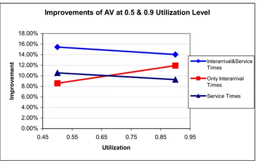
Figure 3.3 Graph of the Overall Results of AV for both Utilization Levels 39

Figure 3.4 Illustration of the Monotone Relationship between the Interarrival Times and Time In System 40

Figure 3.5 Graph of the Overall Results of LHS for both Utilization Levels 46

Figure 3.6 Overall Results of PS at each level when Service Time is the Stratification Variate 52

Figure 3.7 Comparison of CV and PS when Service Time is the Control and the Stratification Variate 54

Figure 3.8 Comparison of AV and LHS 54

Figure 3.9 Comparison of CV+AV and CV+LHS 62

Figure 4.1 Illustration of the Serial Line Production System of Five Stations 63

Figure 4.2 Warm up Period for the Serial Line Production System 64

Figure 5.1 Warm up Period for the (s,S) Inventory Model 82

(10)

Table 2.1 Illustration of the Uniform Random Numbers used in AV 9

Table 2.2 An Example for AV 12

Table 2.3 Illustration of the Uniform Random Numbers used in LHS 13

Table 2.4 Illustration of the Implementation of LHS 17

Table 2.5 An Example for LHS 17

Table 2.6 Replication Averages for Control Variate and Response Variable in CV 24

Table 2.7 An Example for CV 24

Table 2.8 Sethi’s Optimal Stratification Scheme for a Standard Normal Variate 27

Table 2.9 Replication Averages for Stratification Variate and Response Variable in PS 28 Table 2.10 An Example for PS 28

Table 3.1 List of Single and Integrated VRTs that will be Applied to M/M/1 30

Table 3.2 Theoretical Values of Queuing Statistics from the Queuing Theory 31

Table 3.3 Results of the Ten Experiments with the Stream and Initial Seed Numbers for 0.9 Utilization 33

Table 3.4 Results of the Ten Experiments with the Stream and Initial Seed Numbers for 0.5 Utilization

33

Table 3.5 Benchmark Half Length and Standard Deviation Values for 0.9 Utilization 33

Table 3.6 Benchmark Half Length and Standard Deviation Values for 0.5 Utilization 33

Table 3.7 Stream Numbers and Initial Seed Values for AV 34

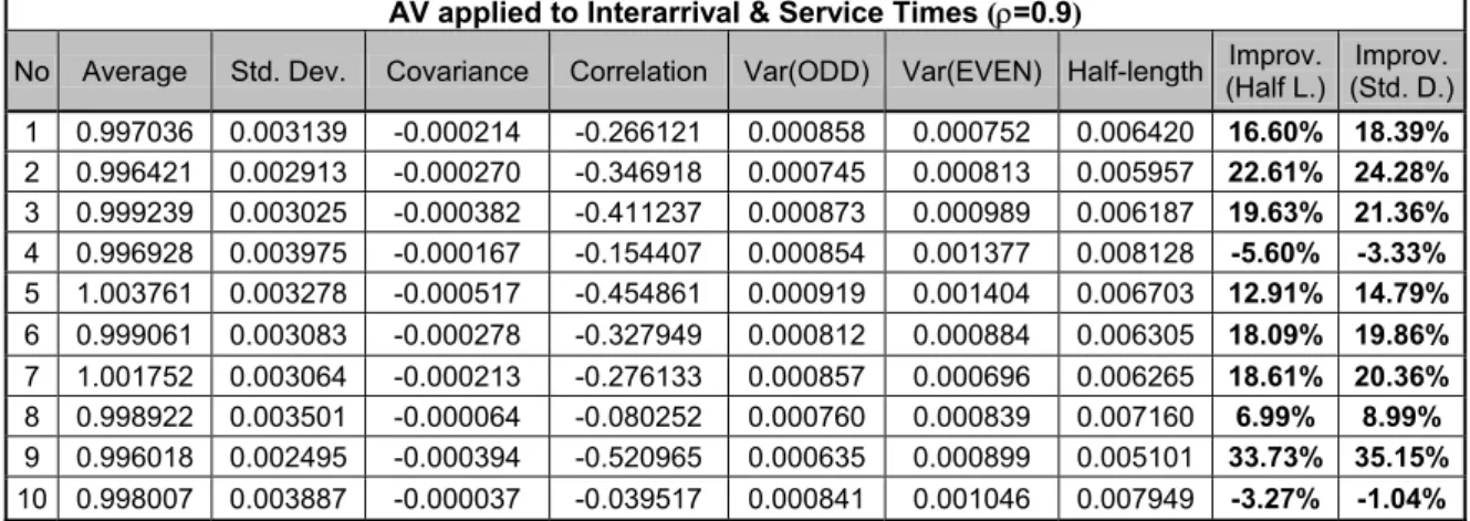
Table 3.8 Results of AV applied to both Interarrival and Service Times for 0.9 Utilization 35 Table 3.9 Results of AV applied to both Interarrival and Service Times for 0.5 Utilization 35 Table 3.10 Confidence Intervals for Improvements when AV applied to Interarrival and Service Times 35

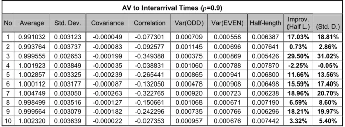
Table 3.11 Results of AV applied to Interarrival Times Only for 0.9 Utilization 37

Table 3.12 Results of AV applied to Interarrival Times Only for 0.5 Utilization 37

Table 3.13 Confidence Intervals for Improvements when AV applied to Interarrival Times Only 37

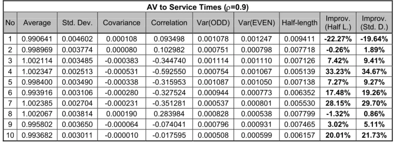
Table 3.14 Results of AV applied to Service Times Only for 0.9 Utilization 38

Table 3.15 Results of AV applied to Service Times Only for 0.5 Utilization 38

Table 3.16 Confidence Intervals for Improvements when AV applied to Service Times Only 38 Table 3.17 Overall Results of AV for both Utilization Levels 39

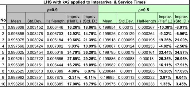
Table 3.18 Stream Numbers and Initial Seed Values for LHS 41 Table 3.19 Results of LHS with k=2 when applied to both Interarrival and Service Times 41

(11)

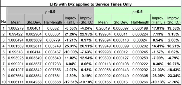
Table 3.21 Results of LHS with k=2 when applied to Service Times Only 42

Table 3.22 Confidence Intervals for Improvements when LHS with k=2 applied to Service Times Only 42

Table 3.23 Results of LHS with k=2 when applied to Interarrival Times Only 43

Table 3.24 Confidence Intervals for Improvements when LHS with k=2 applied to Interarrival Times only 43

Table 3.25 Results of LHS with k=3 when applied to both Interarrival and Service Times 44 Table 3.26 Confidence Intervals for Improvements when LHS with k=3 applied to Both Interarrival and Service Times 44

Table 3.27 Results of LHS with k=3 when applied to Service Times Only 45

Table 3.28 Confidence Intervals for Improvements when LHS with k=3 applied to Service Times Only 45

Table 3.29 Results of LHS with k=3 when applied to Interarrival Times Only 45

Table 3.30 Confidence Intervals for Improvements when LHS with k=3 applied to Interarrival Times only 46

Table 3.31 Overall Results of LHS for both Utilization Levels 46

Table 3.32 Overall Results of AV and LHS for both Utilization Levels 47

Table 3.33 Results of CV for 0.9 Utilization Level 48

Table 3.34 Results of CV for 0.5 Utilization Level 48

Table 3.35 Confidence Intervals for Improvements by CV 48

Table 3.36 Results of PS and Confidence Intervals for Improvements at each Stratification Level obtained with Optimal Allocation Scheme 50

Table 3.37 Results of PS and Confidence Intervals for Improvements at each Stratification Level obtained with Equal Length Scheme 51

Table 3.38 Overall Results in Half Length and Standard Deviation by Each Technique for 0.9 Utilization 52

Table 3.40 Results of the First Combination Scheme of AV and CV for both Utilizations 55

Table 3.41 Results of the Second Combination Scheme of AV and CV for 0.9 Utilization 56

Table 3.42 Results of the Second Combination Scheme of AV and CV for 0.5 Utilization 56

Table 3.43 Results of the Third Combination Scheme of AV and CV for 0.9 Utilization 56

Table 3.44 Results of the Third Combination Scheme of AV and CV for 0.5 Utilization 57 Table 3.45 Confidence Intervals for Improvements by Second and Third Combination

(12)

Table 3.47 Results of CV and LHS with k=3 for both Utilization Levels 59

Table 3.48 Confidence Intervals for Improvements by CV and LHS with k=2 59

Table 3.49 Confidence Intervals for Improvements by CV and LHS with k=3 59

Table 3.50 Individual Improvements in Half Length and Standard Deviation 60

Table 3.53 Overall Improvements of Combinations in Half Length and Standard Deviation for 0.9 Utilization 61

Table 3.54 Overall Improvements of Combinations in Half Length and Standard Deviation for 0.5 Utilization 62

Table 4.1 List of Single and Integrated VRTs that will be Applied to Serial Line Production System 64

Table 4.2 Results of the Ten Independent Replications with the Stream and Initial Seed Numbers 65

Table 4.3 Benchmark Half Length and Standard Deviation Values 65

Table 4.4 Results of AV applied to All Service Times 66

Table 4.5 Confidence Intervals for Improvements when AV applied to All Service Times 66 Table 4.6 Individual Improvements in Half Length and Standard Deviation by AV 67

Table 4.7 Confidence Intervals for Improvements in Half Length and Standard Deviation by AV 67

Table 4.8 Stream and Initial Seed Numbers for LHS 68

Table 4.9 Results of LHS with k=2 when applied to All Service Times 68

Table 4.10 Confidence Intervals for Improvements in Half Length by LHS with k=2 and k=3 68

Table 4.11 Confidence Intervals for Improvements in Standard Deviation by LHS with k=2 and k=3 68

Table 4.12 Comparison of AV and LHS in terms of Half Length and Standard Deviation Improvement 69

Table 4.13 Results of CV and Confidence Intervals for Improvements in Half Length when Different Service Times are used as Control Variates 70

Table 4.14 Confidence Intervals for Improvements in Standard Deviation when All Service Times are taken as Control Variates 70

(13)

Table 4.16 Confidence Intervals for Improvements in Standard Deviation by PS at each

Stratification Level obtained with Equal Probability Scheme 72

Table 4.17 Overall Improvements in Half Length and Standard Deviation by Each Technique alone 73

Table 4.18 Individual Improvements in Standard Deviation for the First Scheme 75

Table 4.19 Confidence Interval for the Improvements in Standard Deviation by the First Scheme 75

Table 4.20 Results of the Second Combination Scheme and Confidence Intervals for Improvements When Different Service times are taken as Control Variates 75

Table 4.21 Results of the Third Combination Scheme and Confidence Intervals for Improvements When Different Service Times are taken as Control Variates 76

Table 4.22 Confidence Intervals for Improvements in Standard Deviation by CV When Different Service Times are taken as Control Variates 76

Table 4.23 Results of CV and LHS with k=2 and Confidence Intervals for Improvements in Half-length for different Control Variates 77

Table 4.24 Results of CV and LHS with k=3 and Confidence Intervals for Improvements in Half-length for different Control Variates 78

Table 4.25 Confidence Intervals for Improvements in Standard Deviation by LHS with k=2,3 and CV when different service times are taken as Control Variates 78

Table 4.26 Overall Improvements in Half Length and Standard Deviation by Each Technique alone 79

Table 4.27 Overall Improvements of Combinations in Half Length and Standard Deviation 79 Table 5.1 List of Single and Integrated VRTs that will be Applied to (s,S) Inventory Model 82

Table 5.2 Results of the Ten Independent Replications with the Stream and Initial Seed Numbers 83

Table 5.3 Benchmark Half Length and Standard Deviation Values 83

Table 5.4 Results of AV 84

Table 5.5 Confidence Intervals for Improvements by AV 84

Table 5.6 Individual Improvements in Half Length and Standard Deviation by AV 84

Table 5.7 Confidence Intervals for Improvements in Half Length and Standard Deviation by AV 84

Table 5.8 Stream and Initial Seed Numbers for LHS 85

Table 5.9 Results of LHS with k=2 and k=3 85

(14)

Table 5.11 Confidence Intervals for Improvements in Standard Deviation by LHS with k=2

and k=3 85

Table 5.12 Comparison of AV and LHS in terms of Half Length and Standard Deviation

Improvement 86

Table 5.13 Results of CV 86 Table 5.14 Confidence Intervals for Improvements in Half Length and Standard Deviation 87 Table 5.15 Results of PS and Confidence Intervals for Improvements at each Stratification

Level obtained with Optimal Allocation and Equal Probability Schemes 88

Table 5.16 Confidence Intervals for Improvements in Standard Deviation by PS at each

Stratification Level obtained with Optimal Allocation and Equal Probability Schemes 88

Table 5.17 Overall Improvements in Half Length and Standard Deviation by Each

Technique alone 89

Table 5.18 Individual Improvements in Standard Deviation for the First Combination

Scheme 90

Table 5.19 Confidence Interval for the Improvements in Standard Deviation by the First

Scheme 90

Table 5.20 Individual Improvements in Half Length and Standard Deviation for the Third

Scheme 90

Table 5.21 Confidence Intervals for the Improvements in Half Length and Standard

Deviation by the Third Combination Scheme 90

Table 5.22 Results of CV and LHS with k=2 for Improvements in Half Length and

Standard Deviation 91

Table 5.23 Results of CV and LHS with k=3 for Improvements in Half Length and

Standard Deviation 91

Table 5.24 Confidence Intervals for Improvements in Half Length and Standard Deviation

by CV+LHS, k=2 91

Table 5.25 Confidence Intervals for Improvements in Half Length and Standard Deviation

by CV+LHS, k=3 91

Table 5.26 Overall Improvements in Half Length and Standard Deviation by Each

Technique alone 92

Table 5.27 Overall Improvements of Combinations in Half Length and Standard Deviation 92

(15)

Chapter 1 Introduction and Literature Review

1.1. Introduction

Analytical methods may not be available or difficult to apply all the time in order to analyze the complex systems including stochastic input variables. In that case, numerical methods are recommended in order to analyze or at least to get an idea about the system behavior or performance. In this context, simulation has a widespread usage with the increasing availability and the capability of the computers. Thus currently it is one of the mostly used tools in practical cases. Simulation is the process of designing a model of the real system and conducting experiments with this model for the purpose of understanding the behaviour of the system and/or evaluating various strategies for the operation of the system (Pegden, Shannon and Sadowski [27])

Since the random inputs to any simulation model produce random outputs, further statistical analysis is required to better interpret the results of the simulation. In this manner, simulation just gives an estimate for each output variable and this estimate is calculated with some error depending on the purpose of the study and the desired precision. One way to increase the precision of the estimators is to increase the sample size. However, this may require a large amount of computational time and effort. Another way is the usage of some methods that provide the same precision with less simulation runs or result in more precision with the same number of simulation runs. Even though it may be sometimes very costly to reach satisfactory results, various techniques have been developed in order to decrease the anticipated cost.

(16)

Variance Reduction Techniques (VRTs) are experimental design and analysis techniques used to increase the precision of estimators without increasing the computational effort or to get the desired precision with less effort. A more statistical definition says that they are the techniques defining a new estimator, which has the same expectation as the default estimator but has a lower variance. That is, these techniques create a new unbiased estimator expected to have a lower variance than the default estimator. Biased estimators can be used in some cases as well (Schmeiser [31]). In those cases, the aim is to obtain a reduction in the mean square error (MSE).

Many VRTs have been developed since the beginning of the computers for the purpose of simulating a system. However, these methods require a thorough understanding of the model being simulated, or at least understanding of some relationships existing between the input and output random variables. In addition, as we will show throughout our experiments, the amount in the variance reduction cannot be predicted in advance and sometimes they can backfire and thus even a higher variance is obtained. Thereby some pilot runs of the simulation can be very useful not only to understand the relationships between the input and output random variables but also to guess the possible reduction in the variance that may be achieved by the application of the VRT.

Many studies focusing on the new methods or the classification of the methods have been made in the literature. Comprehensive surveys are available on the VRTs. A recent survey by L’Ecuyer [16] includes an overview of the techniques, efficiencies of those techniques and the related examples in the literature.

In this thesis, we will focus on four methods and their combinations. Namely, these are Antithetic Variates (AV), Latin Hypercube Sampling (LHS), Control Variates (CV) and Poststratified Sampling (PS). These methods either individually or in combination will be applied to the simulation results of three systems. Firstly, M/M/1 as the most basic queuing system is taken into account under two different utilization levels. A high utilization level (0.9) is chosen to examine the performances of the four methods and their combinations under highly utilized or variable systems. After that, the same process is performed for a moderately variable system and a lower utilization rate (0.5) is considered. Second, a well-studied system, a serial production system of five stations is taken into consideration. During this study, we assume that all stations have the same service time distribution and allow buffers of three units between the stations. Due to the limited (or finite) buffer spaces, ‘starvation’ and ‘blockage’ of the stations occur in this case as well. Finally, a simple inventory model, a periodic review inventory system controlled by an (s, S) Policy, is selected in order to analyze the behaviour of the four methods and their combinations. In this case, stochastic weekly demands exist and when the inventory

(17)

position falls below the reorder point s, a new order is given with a constant lead time of two weeks.

All of the experiments are conducted using the SIMAN V program in the UNIX environment. The computer program codes for all cases of three systems are given in Appendix A. In these codes, only one model and experimental file are given for each case, i.e. only when Antithetic Variates is applied to interarrival and service times simultaneously.

This thesis is organized as follows. In the next section, we give an overview of the techniques in the literature, however, mostly focus on the relevant literature regarding the four techniques and their combinations. In Chapter 2, we present the experimental results of the single application of the techniques and the integration of the techniques on M/M/1 system and this is followed by the corresponding results of Serial Line Production System and (s, S) Inventory Policy in Chapter 3 and 4, respectively. After giving the detailed results, we discuss the general results at two points throughout each chapter. Finally, this thesis ends with a conclusion and further research directions in Chapter 6. In this chapter, we summarize the main findings and conclusions and recommend directions for further research.

1.2. Literature Review

Available literature on VRTs can be classified into three categories as shown below: i. Survey Papers on VRTs and the classification efforts of different VRTs.

ii. Papers introducing new but generally model specific estimators with lower variances.

iii. Papers comparing different VRTs and their combinations in terms of the implementation in different systems and discussing the related results.

A paper by L’Ecuyer [16] consists of an overview of the main techniques in VRT literature and gives some examples regarding those techniques. In general, main techniques existing in the literature can be summarized as follows: Common random numbers, antithetic variates, control variates, importance sampling, indirect estimators, stratification, latin hypercube sampling, conditioning, descriptive sampling, hybrid method, and virtual measures. In addition, some other comprehensive survey papers include Nelson [22] [23], Heidelberger [11], James [12], and Wilson [37].

The first category provides a guide in order to determine the appropriate VRTs and to eliminate the confusion concerning the characteristics of and the relations among VRTs. In this manner, Nelson and Schmeiser [25] present a commendable classification of VRTs. According to their definition, VRTs transform the simulation models into related models that result in more precise estimates of the parameters of interest. These transformations may modify the inputs of

(18)

a simulation model through distribution replacement or dependence induction as well as may transform the outputs through sample allocation or an equivalent allocation. Also, they may modify the statistics through auxiliary information or equivalent information. These basic transformations later extended in order to make taxonomy of VRTs by Nelson [23] and Nelson and Schmeiser [25]. James [12] approaches this subject in a very different way than Nelson [23], and Nelson and Schmeiser [25] [26] did.

Regarding the second category, Calvin and Nakayama [7] proposed new estimators of some performance measures obtained using regenerative simulations of discrete time markov chain. Moreover, new estimators for the queuing systems are proposed by Law [18].

In the final category, comparisons of different techniques regarding their implementation and efficiency and their combination are taken into account. Nevertheless, these comparisons are performed on very few systems since the techniques are model specific. Therefore, the results obtained via those studies are applicable to related models and the application in other systems may even produce worse results. Also, the comparisons of the single and combined methods are not considered thoroughly in the current literature. The rest will be comprised of a brief summary of these studies.

The first class of the applications and the comparison of different VRTs include the comparison of the single techniques. Glynn and Whitt [10] investigate the asymptotic efficiency of estimators time average queue length L and average waiting time W. They show that an indirect estimator for L using the natural estimator for W and the arrival rate λ is more efficient than a direct estimator for L. This is based on the assumption that the interarrival and waiting time in queue are negatively correlated. Furthermore, they indicate that the indirect or direct estimation is related to the estimation using nonlinear control variables.

Carson and Law [8] focus on the efficient estimation of mean delay in queue, mean wait in system, time average number in queue, time average number in system, and time average amount of work in system for simulated queuing systems of GI/G/s for s=1, 2, and 4. Moreover, Law [18] compares the six efficient estimators for queuing system simulations in terms of efficiency through their variance of the asymptotic distribution of the estimator and variance reduction. He indicated that it is more efficient to estimate the performance means using an estimate of mean delay or waiting time in queue than estimating them directly while the latter is more efficient in single server queuing systems. In addition, based on his empirical studies, using the former estimator is more efficient for GI/G/1 queues whereas the latter seems to perform better in GI/G/2 systems.

Minh [21] proposes the partial conditional expectation technique derived from the conditional expectation technique. He points out that the estimator in this technique is

(19)

consistent, unbiased and its variance is smaller compared to the crude estimator. Even though the variance reduction achieved by the new technique may not be as much as by conditional expectation but its applicability to some problems to which conditional technique is difficult to apply makes it advantageous.

Cheng [9] compares two different applications of antithetic variates against independent runs for two examples. Then, he finds out that the application of antithetic variates could be very effective if used appropriately. Sullivan et al. [35] investigate the efficiency of the antithetic variate simulation for estimating the expected completion time of the stochastic activity networks. They figure out that antithetic variate could produce the same precision as Monte Carlo simulation but with approximately ¼ computational effort. Avramidis and Wilson [4] propose multiple sample quantile estimators based on antithetic variates and latin hypercube sampling. In addition, the results of the simulation yielding significant reduction in bias and variance are given while the estimation of the quantiles of a stochastic activity networks.

Ahmed et al [1] show that using infinite source and ample server models as control variates for finite source finite server models can be effective in reducing the variance of sensitivity estimates like gradients and Hessians in repairable item systems. Bauer et al. [5] propose a new procedure in order to use control variates in multi-response simulation if the covariance matrix is known. They also present the results of the applications to closed queuing networks and stochastic activity networks.

Wilson and Pritsker [38] give empirical results on the amount of the variance reductions for queuing simulations when the control variates and poststratified sampling are used separately. According to their results, for analytically tractable models of closed and mixed machine repair systems, posstratification produces variance reduction between 10% and 40% and reductions in the half-length between 1% and 20%. In the control variates case, these reductions are between 20% and 90% for variance and 10% and 70% for half-length. Saliby [30] focuses on descriptive sampling that is stated as an improvement over latin hypercube sampling. They gave an example of the application and the comparison of two methods and indicated that descriptive sampling gave better results. Ross [29] indicates how certain VRTs can be efficiently employed during the analysis of the queuing models. He considered three techniques: dynamic stratified sampling, utilization of multiple control variates, and the replacement of random variables by their conditional expectations.

After that, the literature concerning the application of integrated VRTs. Schruben and Mangolin [32] provides the conditions under which the techniques of antithetic variates and common random numbers produce guaranteed efficiency improvements. Kleijnen [14] combines the antithetic variates and common random numbers in order to compare the two

(20)

alternative systems. He indicated that some implementations of the combined technique could be inferior to antithetic variates or common random numbers individually. Then, he proposes a new combination scheme and experimentally shows the superiority of his scheme to either technique used alone.

Yang and Liou [40] show that the integrated control variates estimated with antithetic variates results in unbiased with smaller variance than the conventional control variate estimator applied without Antithetic Variates. They also prove that the proposed integrated estimator is optimal among the three integrated estimators including the proposed integrated estimator. Kwon and Tew [15] present three methods to combine antithetic variates and control variates which are based on whether the control variates or non-control variates are generated with antithetic variates or not. They indicated that the combined method III, which induces negative correlation among all control and non-control variates, was optimal. Burt and Gaver [6] combine antithetic and control variates and experimentally observed that the combination gave better than the either method applied individually.

Nelson [24] discusses the efficiency of the control variates and antithetic variates in improving the performance of point and interval estimators in the presence of bias due to the determination of the initial bias. Tew and Wilson [36] incorporated control variates into antithetic variates and common random numbers scheme and investigated the conditions under which the combination scheme performed better than antithetic variates and common random numbers, control variates used alone, and direct simulation.

Avramidis and Wilson [2] examined the all pairings of conditional expectation, correlation induction (antithetic variates and latin hypercube sampling) and control variates. Also, they established the sufficient conditions under which that strategy would yield a smaller variance than its constituents would yield individually. They experimented with the stochastic activity networks and indicated that the integrated technique of conditional expectation and latin hypercube sampling performed best.

In this part, some general studies about the VRTs and their integration have been considered. Nevertheless, in the next chapter, we will also mention about the papers specific to each technique.

According to above overview, in general, the literature about the integrated methods is not so intense and as seen most of the studies are devoted to specific models and specific VRTs. Therefore, in this research, we will focus on two other systems (Serial Line Production System and (s,S) Inventory Policy in addition to simple M/M/1 system) and examine the results of the four methods (Antithetic Variates, Latin Hypercube Sampling, Control Variates, and Poststratified Sampling) on these systems. Our study can be classified as in the third category,

(21)

which includes the researches comparing different VRTs and their combinations in terms of the implementation in different systems and discussing the related results. In this manner, we select those four methods since they were not analyzed thoroughly on different systems.

Our study examines the behaviour of the stand-alone and integrated applications of these methods on one commonly (M/M/1) and two uncommonly used (serial line production system and (s,S) inventory policy) systems. We investigate the reasons behind the success or failure of a technique in a specific system and why the combined techniques perform better than the stand-alone applications. 10 different experiments are performed during the applications of the methods individually or in combination to a system in order to increase the reliability of our conclusions. With these 10 experiments, we construct a confidence interval for the average performances of the techniques.

(22)

Chapter 2 Variance Reduction Techniques (VRTs)

The four methods used in this research are Antithetic Variates (AV), Latin Hypercube Sampling (LHS), Control Variates (CV), and Poststratified Sampling (PS). These methods, which are applicable to the simulation of a single system, can be classified into two groups:

1. Methods that try to induce a correlation among the simulation runs in order to reduce

the variance: AV and LHS. In addition, these methods can be considered as dealing

with the input part of the simulation.

2. Methods that use the auxiliary variables for variance reduction: CV and PS. Moreover, CV and PS can be considered as dealing with the output part of the simulation.

During the simulation of a Single System, we just try to increase the precision of the estimated performance measure.

2.1. Antithetic Variates (AV)

Antithetic Variates (AV) modifies the input variables in order to reduce the variance. In other words, AV tries to reduce the variance through inducing a negative correlation by using complementary random numbers among the replications. If

U

is a particular random number (uniform between 0 and 1) used for a particular purpose in the first run, we use

1

for the same purpose in the second run. That is, a “small” observation in the first run tends to be offset by a “large” observation in the second run.

k

U

(23)

In this manner, we double the number of runs and average the consecutive odd and even numbered replications to get a smaller variance. As indicated more clearly in the Table 2.1, if 0.153 is used to generate a service time in the first replication, 1-0.153=0.847 is used in the second replication to generate the same service time. By this way, we make the first and the second replications correlated while no dependence occurs with the other pairs.

Rep 1 Rep 2 Rep 3 Rep 4 … Rep 2n-1 Rep 2n 0.153 0.847 0.697 0.303 … 0.326 0.674 0.631 0.369 0.159 0.841 … 0.455 0.545 0.741 0.259 0.342 0.658 … 0.112 0.888 … … … ) 1 ( 1

X

(2) 1

X

(1) 2

X

(2) 2

X

_…

X

n(1) ) 2 ( n

X

X1 X2 … Xn

Table 2.1 Illustration of the Uniform Random Numbers used in AV

As illustrated better in the Figure 2.1, the desired performance measure is estimated for each pair of runs, which are ( (1), (2)).

j j X X Negatively Correlated Replications Pair 1:

X

₁(1) (2) 1

X

₁ Pair 2:

X

₂(1) (2) 2

X

X₂ … … … … Pair n:

X

_n(1) (2) n

X

_n Independent

)

(n

X

Figure 2.1 Illustration of the Negatively Correlated Replications in AV

Then, taking the average of the two runs in each pair, we calculate the corresponding average performance measures, X_j’s, for each pair:

2 ) 2 ( ) 1 ( j j j X X X = +

There exist no dependence between the pairs, hence, replications in different pairs and the averages of the pairs are perfectly independent. Within each pair, complementary random numbers are used for the same purpose by performing synchronization appropriately. More

(24)

specifically, we use U’s in the (1) for a specific purpose and

j

X 1−U ’s for the same purpose in

the X(_j2).

After that, can be assumed to be generated from independent replications and thus the same procedure as in the independent case is followed in order to construct a confidence interval. Assume that the average of ’s is

) ,.., , (X₁ X₂ X_n n j X

X

(n

)

. Hence,

X

(n

)

is an unbiased estimator of the desired performance measure:

) ( ) ( ) (_X() _E _X _X _n E i _j j = = = µ

Consequently, 100(1−α)% confidence interval around the mean

E

(

X

(

n

))

is constructed as follows:

))

(

.

)

(

n

t

₁_,₁ _/₂

Var

X

n

X

µ

_n₋ ₋_α

Degrees of freedom should be taken as

n

−

1

where

n

is the total number of macro replications while constructing the confidence interval.

The mathematical basis for this method is based on a very simple statistical formula:

) 1 ( 2 ) ( 4 ) . ( 2 ) ( ) ( ) ( )] ( [ ) 1 ( ) 2 ( ) 1 ( ) 2 ( ) 1 ( ρ + = + + = = n X Var n X X Cov X Var X Var n X Var n X Var j j j j j j ,

where

ρ

is the correlation between the negatively correlated replications. As it can be seen in the above formula, if the two runs within a pair are made independently, then covariance part will be zero, however, if negative correlation can be induced between the two random variables then covariance part will be negative. Thus the overall variance will be reduced as intended by AV. In another perspective, based on the last part of the above formula, antithetic variate estimator based on pairs of simulation runs should be more precise than the classical Monte Carlo estimator based on independent replications when

n

2

ρ

<

0

.

Synchronization (i.e., usage of 1-U’s for the same purpose U’s used) of the input random variables becomes an important issue during the application of AV. Otherwise, the benefit due to the intended negative correlation among the replications may be lost. Law and Kelton [19] mentions some programming tricks about the synchronization of the random variables such as random-number stream dedication, using the inverse-transform method of variate generation wherever possible, judicious wasting of random numbers, pre-generation, and advancing the stream numbers across multiple replications.

Improper synchronization of the input random numbers can cause an increase in the variance of the desired performance measure. Law and Kelton [19] state that unless synchronization is provided appropriately, AV can even backfire; variance of the desired

(25)

performance measure can even increase. Full synchronization of the all input random variables may not be possible in some large simulation models due to the limited number of seeds available in today’s most popular simulation packages. Nevertheless, by determining the most crucial variables in the simulation models and inducing negative correlation among those variables, AV can still be a very useful tool to reduce the variance. A very simple guideline to create negatively correlated replications could be to choose the input variables that affect the desired performance measure significantly. These can be determined through some pilot runs of the simulation model beforehand.

Although AV can be very effective in some cases, its effectiveness is not always guaranteed; we do not know whether AV will reduce the variance and if so, how much the reduction will be. In order to apply AV successfully, the output or response variable is required to be a monotone function of the random variables used to produce the random variates. If the response variable is a monotone function of its arguments, then as shown in Ross [28], the covariance between the complementary replications will be negative. Hence, this negative correlation will help to reduce the variance. In this context, therefore, the Inverse Transform Method is suggested to generate the random variates whenever possible. Using this method, the random variables become a monotone function of the uniform random variates and this is theoretically sufficient for AV to provide a reduction in the variance. For instance, in M/M/1 system since interarrival and service times can be generated using Inverse Transform Method, AV can be effective in reducing the variance of the Time-in-system statistics. However, the magnitude of the reduction still cannot be predicted in finite sample cases in advance.

Example 1. Antithetic Variates (AV)

Consider the simple M/M/1 system with an arrival rate of 9 per minute and service rate of 10 per minute. Suppose that we want to get an estimate of the expected Time-in-system statistics using simulation and we desire the estimator as precise as possible. Using independent sampling with 20 replications, we get the half-length as 0.0547 (by using the estimates of the mean and the standard deviation and applying the common formula for confidence interval with appropriately chosen degrees of freedom), which is not precise as we desire. Hence, we may use a variance reduction technique in order to increase the precision. In this case, 20 replications, of which consecutive odd and even numbered replications are correlated, are taken in order to get 10 independent replications. Negative correlation is induced between both the interarrival and service times. After that we take the average of time-in-system statistics in those correlated replications as indicated in the Table 2.2:

(26)

Rep # ODDS

Time-in-system Rep # EVENS

Time-in-system AVERAGE Average Time-in-system 1 X11 0.927 2 X12 1.031 X1 (0.927+1.031)/2= 0.9790 3 X21 0.907 4 X22 1.048 X2 (0.907+1.048)/2= 0.9775 5 X31 0.982 6 X32 1.136 X3 (0.982+1.136)/2= 1.0590 7 X41 1.038 8 X42 0.945 X4 (1.038+0.945)/2= 0.9915 9 X51 0.899 10 X52 0.907 X5 (0.899+0.907)/2= 0.9030 11 X61 1.028 12 X62 0.991 X6 (1.028+0.991)/2= 1.0095 13 X71 0.925 14 X72 0.992 X7 (0.925+0.992)/2= 0.9585 15 X81 0.979 16 X82 0.941 X8 (0.979+0.941)/2= 0.9600 17 X91 1.026 18 X92 0.935 X9 (1.026+0.935)/2= 0.9805 19 X101 1.098 20 X102 0.888 X10 (1.098+0.888)/2= 0.9930

Table 2.2 An Example for AV

According to these values, Vˆar(X_i₁)=0.0044, Vˆar(X_i₂ )=0.0056, and 001834 . 0 ) X , X ( ov

Cˆ _i₁ _i₂ =− . Using these data and the knowledge from the statistics,

00016

.

0

10

4 )

001834

.

0 (

2 0056

.

0 0044

.

0 )

(

ˆ

4 )

,

(

ˆ

2 )

(

ˆ

)

(

ˆ

)

(

ˆ

9812

.

0 )

9930

.

0 9805

.

0 ...

9775

.

0 9790

.

0 (

10

1

2 1 2 1

=

×

−

×

+

=

⇒

×

+

=

+

×

=

X

ar

V

n

X

ov

C

X

ar

V

X

ar

V

X

ar

V

X

i i i i

a 95% confidence interval around the mean is (t9, 1-0.025=2.26):

].

1 ;

9526

.

0 [

0286

.

0 9812

.

0 00016

.

0 9812

.

0 µ t

₉_,₁₋₀_.₀₂₅

×

=

µ

=

As a result, reduction in CI compared to independent sampling case is % 71 . 47 0547 . 0 0286 . 0 0547 . 0 = −

2.2. Latin Hypercube Sampling (LHS)

LHS is also based on a correlation induction scheme; it generates negatively correlated micro replications in order to get a single macro replication. This idea is actually similar to AV and LHS can be considered a more general form of AV. AV uses only two micro replications to get one macro replication while LHS can use more than two negatively correlated micro replications. LHS can be considered as a transformation to redefine the inputs of a simulation model by inducing dependence. It works in a very similar way to AV. The average of

k

output variables from correlated micro replications is used to construct confidence intervals.

(27)

Synchronization of the input random numbers is necessary to obtain correlated micro replications.

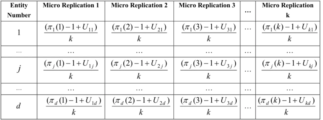
LHS generates the correlated micro replications that are induced in

d

dimensions according to the following formula:

k

U

i

U

i j ij j

+

−

=

(

)

1

) (

π

for

i 1

=

,...,k

and

j 1

=

,...,d

, where π₁(.),...,π_d(.) are permutations of the integers

{

}

that are randomly sampled with replacement from the set of such permutations. denotes the th element in the ’th sampled permutation and

U

k

,...,

2 ,

1 )

(i

j

π

!

k

ij

i

j

values are uniform random

numbers between 0 and 1. Also,

U

is the ’th input random number used in the

i

’th replication. As seen in the above formula and the table below, LHS wastes many random numbers as compared to AV and thus it requires much more time and effort. In general, the input random numbers in LHS can be represented as in Table 2.3.

ij

j

Entity Number

Micro Replication 1 Micro Replication 2 Micro Replication 3

… Micro Replication k 1 k U ) 1 ) 1 ( (π₁ − + ₁₁ k U ) 1 ) 2 ( (π₁ − + ₂₁ k U ) 1 ) 3 ( (π₁ − + ₃₁ … … … … … … …

j

k U _j j(1) 1 ) (π − + ₁ k U _j j(2) 1 ) (π − + ₂ … … … … … … … d k U _d d(2) 1 ) (π − + ₂ … k U k) 1 _k ) ( (π₁ − + ₁ k U _j j(3) 1 ) (π − + ₃ k U k _kj j( ) 1 ) (π − + k U _d d(1) 1 ) (π − + ₁ k U _d d(3) 1 ) (π − + ₃ k U k _kd d( ) 1 ) (π − +

Table 2.3 Illustration of the Uniform Random Numbers used in LHS

The essence of LHS is the independent generation of random permutations and uniform random numbers. In this manner, for each random number, a stratified sample of size is taken from a uniform distribution on [0,1] so that observations within the sample and observations in each stratum are negatively correlated. LHS generates the random variates using those negatively correlated random numbers and the Inverse Transform Method.

k

In LHS, the region between 0 and 1 is divided into non-overlapping intervals of equal length for each random variable. Hence,

k

different values in the non-overlapping intervals are selected randomly for each random variable so that one value from each interval is generated. In this way, we ensure that the input random variable has all portions of its

k

(28)

distribution. Hence, if an input random variable in one replication uses a uniform number from a region for a specific purpose, then in other negatively correlated replications, same input random variable is forced to use another uniform random number from the other regions. For

, ’th region can be considered as

,...,k

i

=

1 i









 −

=

k

i

k

i

R

_i

1 ,

which simply follows from the method of generating uniform random numbers in LHS.

In this method, we take

n

replications in total as micro replications are taken for one macro replication. Then, we calculate average of each macro replication using the averages of the micro replications. As illustrated in the Figure 2.2, the desired performance measure is estimated for each pair of runs, which are .

k

.

k

) ) ,.., , ( (1) (2) (k j j j X X X Macro Replication 1:

X

₁(1) (2) … 1

X

( ) 1 k

X

₁ Macro Replication 2:

X

₂(1) (2) … 2

X

( ) 2k X X₂ … … … … … … Macro Replication n:

X

_n(1) (2) … n

X

(k) n X

X

_n

)

(

n

X

Independent Micro Replications (Negatively Correlated)

Figure 2.2 Illustration of the Negatively Correlated Replications in LHS

Then, taking the average of the each micro replication’s average corresponding to each macro replication, we calculate the corresponding average performance measures, ’s, for each macro replication:

j X k X X X X k j j j j ) ( ) 2 ( ) 1 ( ₊ ₊_...₊ =

Since the selection of the permutations and the uniform random numbers while determining the uniform random number to be used in micro replications are performed randomly, there does not exist any dependency among the micro replications corresponding to different macro replications, hence, micro replications belonging to separate macro replications and thus their averages are perfectly independent.

After that, can be assumed to be generated from independent replications since they are perfectly independent and thus the same procedure as in the

)

,..,

,

(29)

independent case is followed in order to construct a confidence interval. Assume that the average of X_j’s is

X

(

n

)

. Hence,

X

(

n

)

is an unbiased estimator of the desired performance measure,

µ

=

E

(

X

(

n

))

and

µ

=

E

(

X

_j

)

. Consequently, 100(1−α)% confidence interval around the mean

E

(

X

(

n

))

is constructed as follows:

))

)

(

n

t

₁_,

X

µ

_n₋ ₁₋_α_/₂

.

Var

(

X

(

n

While constructing the confidence interval, degrees of freedom should be taken as where is the total number of macro replications.

1 −

n

In fact, LHS is proposed to be more effective than direct simulation provided that the output variable is a monotone function of the input random variables. One advantage of LHS occurs when the output random variable is dominated by a few of input random variables. In this case, applying LHS on all input dimensions assures us that all input variables are represented in a fully stratified manner.

McKay, Beckman, and Conover [20], the originators of LHS, proved that the LHS estimators are unbiased in their original papers. Furthermore, Stein [34] proved that the variance of the estimator is lower compared to simple random sampling. When LHS was firstly proposed by McKay, Beckman, and Conover [20], they assumed that the input random variates were independent and each of these variates was generated using the Inverse Transform method. On the other hand, Avramidis and Wilson [4] generalized LHS so that none of these assumptions were required anymore.

Example 2. Latin Hypercube Sampling (LHS)

Consider the simple M/M/1 system with an arrival rate of 9 per minute and service rate of 10 per minute. Using 30 independent replications, we construct a confidence interval with a half-length of 0.0494. Since d is the number of entities in each simulation run, it is equal to 10,000 in

this case. In this example, we will use Latin Hypercube Sampling in order to reduce the variation around the mean. In order to induce negative correlation around the mean, we will produce service times using negatively correlated uniform random numbers and inverse transformation method. This can be summarized as follows:

Determine the number of correlated replications or level of stratification (k), say k=3. Generate a random permutation of the numbers: 1, 2, 3 (k), say 3-1-2.

Generate three uniform random numbers, say u1=0.5470, u2=0.3450, and u3=0.9365,

(30)

For micro replication 1, use U1=(i-1+u1)/k=(3-1+0.5470)/3= 0.849 to generate an

observation. Similarly, use U2=(i-1+u2)/k=(1-1+0.3450)/3= 0.1150 for micro replication 2

and U3=(i-1+ u3)/k=(2-1+0.9365)/3= 0.6455 for micro replication 3.

Using the above procedure, generate the observations in the simulation run length and collect the required statistics, which is time-in-system in our case.

Calculate the average of the averages of those three correlated micro replications to calculate the corresponding time-in-system value for each macro replication.

After that follow the same procedure in the independent case to calculate the confidence interval and take the degrees of freedom as n-1=10-1=9.

Basic idea of using the above formula to generate input uniform random numbers for micro replications is to choose observations so that while one of the observations is in the low level, one of the other will be in the middle level and the other will be in the high level. That is, if a small service time is generated in the micro replication 1, a large service time is generated in one of the other two replications and a nearly average service time is generated in the last. As illustrated for our case in the Figure 2.3, [0, 1] length is divided to three equal parts and the observations or random variables in the micro replications are forced to use only one of these parts while generating an observation. In this figure, we show that if the permutation turns out to be 1, the input uniform random number is enforced to be in the first interval. The same routine is followed for other permutation values.

3 1 1 1 2 1 1 1 1 1 1 1

1

2

3

2

3

1

3

2

3

1

3

1

3

1

2

3

1

0

3

1

1 R

U

i

R

U

i

R

U

i

∈

⇒

≤

<

⇒

+

=

+

−

=

⇒

=

∈

⇒

≤

<

⇒

+

=

+

−

=

⇒

=

∈

⇒

≤

⇒

=

+

−

=

⇒

=

R3

R2

R1

1 2/3

1/3

0

Figure 2.3 Illustration of the Stratification Idea in LHS

In the Table 2.4, basic mechanism of this procedure is illustrated better for our case. We generate 40,000 uniform numbers and use the given formula to produce the random numbers that will be used to generate the service times in each of three micro replications.

(31)

Uniform R.V.(U)

Random

Permutation Micro Replication 1 Micro Replication 2 Micro Replication 3

Entity No 1 Uu12=0.3450 =0.5470 u3=0.9365 3-1-2 (3-1+0.5470)/3 =_0.8490 (1-1+0.3450)/3 = _0.1150 (2-1+0.9365)/3 =_0.6455 Entity No 2 uu12=0.1180 =0.6424 u3=0.4382 1-3-2 (1-1+0.1180)/3 =_0.0393 (3-1+0.6424)/3 = _0.8808 (2-1+0.4382)/3 =_0.4794 … … … … … … Entity No 40000 u1=0.8760 u2=0.2791 u3=0.7542 2-3-1 (2-1+0.8760)/3 =_0.6253 (3-1+0.2791)/3 = _0.7597 (1-1+0.7542)/3 =_0.2514

Table 2.4 Illustration of the Implementation of LHS

After running the model, we collect the time-in-system statistics for each micro replication as shown in the Table 2.5. Since we generate k=3 correlated micro replications in

order to get one macro replication, 10x3=30 micro replications have been taken for 10 macro replications: j=1,2,3 i Macro Replication 1 Macro Replication 2 Macro Replication 3 Macro Replication 4 Macro Replication 5 Macro Replication 6 Macro Replication 7 Macro Replication 8 Macro Replication 9 Macro Replication 10 Micro i 1 1.07590 0.94422 0.98221 0.93811 0.95893 0.91587 1.03530 0.97252 0.90675 1.03900 Micro i 2 1.00570 1.07700 1.07030 1.03520 0.84605 1.14150 0.95079 1.08260 0.87119 1.02330 Micro i 3 0.98294 0.93460 0.84025 1.05600 0.93333 0.99405 1.13620 0.86528 0.89788 0.95832 Average X1=1.022 X2=0.985 X3=0.964 X4=1.010 X5=0.913 X6=1.017 X7=1.041 X8=0.973 X9=0.892 X10=1.007

Table 2.5 An Example for LHS

After calculating the average time-in-system statistics for each macro replication, we use the same procedure with the independent sampling case and use degrees of freedom as 10-1=9. 2 2

₍

₀

_.

₀₄₈₂

₎

)

9824

.

0 (

9

1 )

(

ˆ

9824

.

0 )

007 .

1 ...

985 .

0

022 .

1 (

10

1 =

−

×

=

+

×

=

∑

X

i

X

ar

V

X

a 95% confidence interval around the mean is

]

0168

.

1 ,

9479

.

0 [

0345

.

0 9824

.

0

10 )

0482

.

0 (

9824

.

0 µ t

₉_,₁₋₀_.₀₂₅

×

2

=

µ

=

As a result, reduction in CI compared to independent sampling case is % 16 . 30 0494 . 0 0345 . 0 0494 . 0 = −