Selçuk J. Appl. Math. Selçuk Journal of Vol. 6. No.2. pp. 9-26, 2005 Applied Mathematics
Arti…cial Neural Networks Approach to Fuzzy Linear Programming Nimet Yap¬c¬Pehlivan1 and Ay¸sen Apayd¬n2
1Department of Statistics, Selcuk University, 42031 Konya, Turkey;
e-mail:nyapici@ selcuk.edu.tr
2Department of Statistics, Science Faculty, Ankara University, Tandogan Ankara,
Turkey
e-mail:apaydin@ science.ankara.edu.tr
Received : May 25, 2005
Summary. Linear Programming (LP) is to maximize or minimize an objective function subject to constraints. Fuzzy Linear Programming (FLP) is a model used in the case of uncertainty in LP. Actually, since the vagueness is an im-portant phenomena in real situations, FLP model is an e¤ective approach to this kind of problems. In recent years, the Arti…cial Neural Networks (ANN) method has been widely used in optimization problems. The main idea in ANN approach is to transform the constraint optimization model into the uncon-straint optimization model. Therefore, complicated or uncertain structures can be easily solved by using an energy function. In this study, FLP models and ANN approach are discussed. ANN approach developed by Wang and Chankong (1992) is used for solving FLP models given in …ve main groups. FLP models are reformulated as LP. ANN approach is used to solve this new LP model. In the last part, the results are discussed by an application.
Key words: Fuzzy Linear Programming, Articial Neural Networks.
1. Introduction
In the real world situations, precise mathematics are not su¢ cient to model a complex system because of incomplete knowledge and information. Fuzzy Set Theory (FST) expresses fuzziness in the narrow sense by means of the concept of sets. FST was developed by Zadeh in 1965 [16]. FST has been applied in many …elds, such as operations research, management science, control theory, arti…cial intelligence / expert sytem [10].
In operations research, FST has been applied to techniques of linear and non-linear programming, dynamic programming, queueing theory, multiple criteria decision making and so on [6]. FLP is generated using the FST and introduced by Zimmermann in 1978. In other words, FLP is a special extension of LP in order to make decision in fuzzy environment. In the LP model, the inputs (c; A; b) or objective function or those combination can be fuzzy. Thus, FLP models have not general forms [6, 16].
ANN is a developed model inspirating from biological neural system. In recent years, ANN has been especially used for optimization problems and also wide-spreadly used for maximization and minimization problems with discrete state space. After proposing ANN approach for LP model by Hop…eld in 1985, Tank and Hop…eld developed this approach in 1986. Wang and Chankong (1992) composed recurrent(=feedback) ANN structure. This structure is especially prefered in LP [12].
The most widely used method for solving LP problems is the simplex method developed by Dantzig in the 1940s [12]. Complex problems give better solutions than linear techniques by using ANN. Therefore, ANN is used for FLP models. In this paper, FLP problems are solved by both simplex method and ANN ap-proach, and the results are compared. This paper consists of …ve sections. Sec-tion 2, contains fuzzy linear programming. SecSec-tion 3, contains arti…cial neural networks and arti…cial neural networks approach to fuzzy linear programming. Section 4, contains applications. Finally Section 5, contains results.
2. Fuzzy Linear Programming
In this paper, …ve FLP models are studied. These models are, LP model with fuzzy right hand sides, LP model with fuzzy parameters in the objective func-tions, LP model with fuzzy right hand sides and objective, LP model with fuzzy right hand sides and coe¢ cient matrix and LP model with all fuzzy coe¢ cients [14].
2.1. Linear Programming Model with Fuzzy Right Hand Sides This model is formulated as follows.
(1)
M ax Z = cx
(Ax)i6 ~bi i = 1; 2; :::; m
xj> 0 j = 1; 2; :::; n
where ~bi (i = 1; 2; :::; m) are in [bi; bi+ pi] with given pi. pi’s are tolerance for
each fuzzy constraint and assumed known.
Verdegay’s Approach: In this approach, membership function is considered as follows. (2) i(x) = 8 < : 1; (Ax)i< bi 1 [(Ax)i bi] pi ; bi6 (Ax)i 6 bi+ pi 0; (Ax)i > bi+ pi
By using equation (2), equation (1) can be written as
(3)
M ax Z = cx
(Ax)i6 bi+ (1 )pi; i = 1; :::; n
x> 0 2 [0; 1]
Equation (3) is equivalent to a parametric programming problem while = 1 [3, 5, 6, 14].
Werners’s Approach: In this approach, because of fuzzy total right hand sides or fuzzy inequality constraint, the objective function of equation (1) should be fuzzy. At …rst, following problems z0and z1 will be solved.
(4) z0= M ax cx (Ax)i6 bi; i = 1; :::; m x> 0 2 [0; 1] (5) z1= M ax cx (Ax)i6 bi+ pi; i = 1; :::; m x> 0 2 [0; 1]
By using the values of z0and z1, the membership functions of objective function
is constructed as, (6) G(x) = 8 > < > : 1; cx > z1 1 (z1 cx)i (z1 z0); z06 cx 6 z1 0; cx < z0
By using Equation (2) and Equation (6), LP model with fuzzy right hand sides can be transformed to
(7) M ax Z = G(x) = 1 (z1 cx) = z1 z0 > i(x) = 1 [(Ax)i bi)]=pi> x> 0 2 [0; 1] [5, 6, 14, 15].
2.2. Linear Programming Model with Fuzzy Parameters in the Objective Func-tion
This model is formulated as,
(8)
M ax Z = ~cx
(Ax)i6 bi i = 1; 2; :::; m
xj> 0 j = 1; 2; :::; n
Verdegay proposed for this problem, that there always exists another one which is dual and has the same fuzzy solution. The dual form of equation (3) is,
(9) M in Z = au a> b + p (, 1 [bi pi] =pi> 1 ; i = 1; :::; m) uAT > c u> 0 2 [0; 1]
where = 1 . Hence, optimal solution u is obtained from solving Equation (9). Then by using u , optimal solution of LP model with fuzzy parameters in the objective function is obtained [6, 14].
2.3. Linear Programming Model with Fuzzy Right Hand Sides And Objective Function
This model is formulated as,
(10)
M ax Z = ~cx
(Ax)i 6 ~bi i = 1; 2; :::; m
xj > 0 j = 1; 2; :::; n
For the solution of Equation (10), an approach is proposed by Zimmermann (1991). In this approach, the goal and its corresponding tolerance of the fuzzy objective are given initially. Fuzzy right hand sides bi (i = 1; 2; :::; m) and
its corresponding tolerance pi are given. The fuzzy objective and the fuzzy
constraints are considered without di¤erence and their corresponding regions can be described in the intervals [bi; bi+ pi] for i = 1; 2; :::; m
For the objective function, membership function is described as follows,
(11) G(x) = 8 > > < > > : 1; cx > bG 1 (bG cx)i pG ; bG pG cx bG 0; cx < bG pG
By using equation (2) and equation (11),
(12) M axZ = G(x) = 1 [(bG cx)] =pG> i(x) = 1 [((Ax)i bi)] =pi> x> 0 2 [0; 1] is obtained [2, 6, 10, 14].
2.4. Linear Programming Model with All Fuzzy Right Hand Sides and Fuzzy Coe¢ cient Matrix
This model is formulated as,
(13)
M ax Z = cx
( ~Ax)i6 ~bi i = 1; 2; :::; m
xj> 0 j = 1; 2; :::; n
In this problem, all fuzzy numbers are assumed triangular and de…ned as A =< aij; lij; rij > and b =< bi; ui; vi >. By using the summation and multiplication
operations on fuzzy numbers, equation (13) can be rewritten as follows
(14) M ax Z = cx n P j=1 aijxj 6 bi; i = 1; :::; m j = 1; :::; n n P j=1 (aij lij)xj6 bi ui n P j=1 (aij+ rij)xj6 bi+ vi xj> 0
In the equation (14), on account of all numbers are real numbers. equation (14) is a classical linear programming problem. For LP model with fuzzy right hand sides and fuzzy coe¢ cient matrix, the solution of this problem is optimal solution x [5, 14].
2.5. Linear Programming Model with All Fuzzy Coe¢ cient This model is formulated as,
(15)
M ax Z = ~cx
( ~Ax)i6 ~bi i = 1; 2; :::; m
xj> 0 j = 1; 2; :::; n
For equation (15), a fully trade-o¤ approach was proposed by Carlsson and Ko-rhonen (1986) [1]. It is assumed that the user can specify the intervals [c0; c1),
[A0; A1) and [b0; b1) for the possible values of the parameters. The lower bound
represents risk-free values, the upper bound represents impossible and the solu-tion obtained by using these values is not implementable values. Moving from risk-free towards impossible parameter value, it can be reached to solutions hav-ing upper membership degrees or for reachhav-ing optimistic solutions the reliable solutions can be used. The task is to …nd an optimal compromise solution. The membership function of parameter c is de…ned as follows,
(16) c= ac[1 expf bc(c c0)(c0 c0)g]
where bcis speci…ed by decision maker. bc > 0 or bc < 0 and ac = 1= [1 exp(bc)]
and c 2 [c0; c1). And
c= 1 when c6 c0, c= 0 when c > c1.
In the same manner, the membership function of the parameters A and b can be obtained. Because of full trade-o¤ between c; A and b, the solution always exists at = c= A= b, therefore, following equations can be obtained
(17) c = gc( ); A = GA( ); b = gb( )
where, 2 [0; 1] and gc; GA; gb are inverse functions of c; Aand b. By using
equation (17), LP model with all fuzzy coe¢ cients can be rewritten as,
(18)
M ax Z = [gc( )] x
[GA( )] x6 gb( )
x> 0
equation (18) is a nonlinear programming model. It can be solved by any LP techniques, if is given [1, 6, 14].
3. Arti…cial Neural Network And Arti…cial Neural Network Ap-proach To Fuzzy Linear Programming
Arti…cial Neural Network can be described as parallel distributed system such that the system is formed by the simple operation units connected to each others with weighted connection [9]. ANN consists of input layer, hidden layer and output layer. In the biological neural network, each dendrit refer to inputs, each synapse refer to weights, cell body refer to activation function and each axon refer to outputs in the ANN [4, 7,13].
In the mathematical model of ANN, total potential and output value are calcu-lated as follows respectively,
N ET = n X i=1 xiwi O = F (N ET )
where, xi’s are inputs and wi’s are weights (i = 1; 2; :::; n), is threshold of
neu-ron and F (:) is activation function. The activation function types are, threshold, linear, hyperbolic tangent, sigmoidal and ramp [3, 13]. According to processing state, ANN is parted of feedforward ANN and feedback ANN. In the feedfor-ward ANN, signal direction is one that is input to output, the layer output has no a¤ect on the layer. In feedback ANN, signal direction is input to output. Moreover other neuron can take signals from itself, other neurons in the same layer and the neurons in the other layer’s [8, 11].
Recurrent ANN approach for solving LP models is proposed by Wang and Chankong (1992). In the Wang and Chankong’s ANN approach, the general form of LP problem is described as follows.
(19)
M in Z = cTx Ax = b LB6 x 6 UB
where, A is a coe¢ cient matrix, c is a cost vector, b is a right hand side vector, x is an unknown decision variable vector. LB and UB are lower and upper bounds respectively [12].
The LP solution process consists of two phase. The …rst phase is concerned with problem reformulation. In this phase, a LP problem is reformulated as a penalty problem by incorporating the constraint(s) into an energy function as penalty term, that is,
M in
x2XE(x; ) = c
where, E(x; ): Energy function, p(x): Nonnegative penalty function, : Penalty parameter, X: State space de…ned by LB and UB containing the feasible region
^
X of the LP problem [12].
Energy function and activation function are de…ned as respectively,
E[x(t); (t)] = cTx(t) + (t)(x(t)TATAx(t) 2x(t)TATb bTb)=2) xi(t) = F [ui(t)] = F [ 1 cu t Z 0 [c + ( )(ATAx( ) ATb)p(x( ))d ]
where, cu is a positive capacity parameter. The second phase involves state
stabilization. In this phase, the state of recurrent ANN moves from an initial state toward an equilibrium (steady-state) exists.
ANN approach is proposed by Wang and Chankong (1992) for solving FLP problem. Wang and Chankong’s ANN approach is an algorithm consisting of …ve steps. This algorithm is as follows [12].
Step 1: (Initialization). Input coe¢ cients of the objective function cTx; set initial state x(0) randomly such that (x(0) =2 ^X); select (0) > 0; t > 0 and t = 0.
Step 2: Computing gradient vector.
g(t)= c + (t)(2A4 TAx(t) 2ATb) Step 3: Computing new state.
u(t + t) = u(t) tg(t)[x(t)TATAx(t) 2x(t)TATb bTb]=cup
x(t + t) = F [u(t + t)] Step 4: Adjusting penalty parameter.
(t + t) = (t) + t= x(t)TATAx(t) 2x(t)TATb + bTb =2 c ) Step 5: Checking termination criterion. If x(t + t) = x(t) and (t + t) 6= (t) then stop. Else t = t + t and go to Step 1.
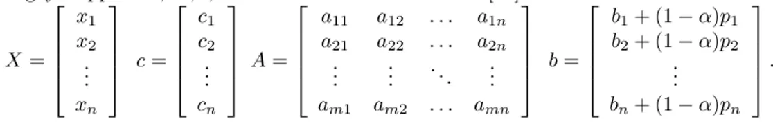
In this paper, we consider …ve FLP models. Each FLP models are remodeled as LP models by using membership functions. We solve new LP models by using Wang and Chankong’s ANN approach. For each FLP models, we described and rearranged parameters A; b and c in the Wang and Chankong (1992)’s ANN approach. Consequently, we rewrited Wang and Chankong’s ANN algorithm for
…ve FLP models. For example; in the LP with fuzzy right hand sides problem Verdegay’s approach, X; c; A and bare de…ned as follows [14]
X = 2 6 6 6 4 x1 x2 .. . xn 3 7 7 7 5 c = 2 6 6 6 4 c1 c2 .. . cn 3 7 7 7 5 A = 2 6 6 6 4 a11 a12 : : : a1n a21 a22 : : : a2n .. . ... . .. ... am1 am2 : : : amn 3 7 7 7 5 b = 2 6 6 6 4 b1+ (1 )p1 b2+ (1 )p2 .. . bn+ (1 )pn 3 7 7 7 5: 4. Application
FLP problems are studied in …ve main groups. For solving these problems, simplex method and ANN approach are used and the results are compared. These problems have two di¤erent structures. Some problems are taken from the literature and some of them are simulated. Owing to nonnegative constraints, the feasible solution …eld of these problems is located in the …rst quadrant of the coordinate plane. Therefore, in the solution process of ANN, activation function Fi[ui] is taken as e ui. The results of problems are given at Table 1-6.
V a r i a b l e s O b j e c t i v e f u n c t i o n P r o b l e m x1 x2 x3 x4 x5 x6 x7 M axZ P 1 S i m p l e x M e t h o d 0 . 0 0 . 2 0 . 5 0 . 8 1 . 0 3 . 0 0 3 . 0 5 3 . 1 2 3 . 2 0 3 . 2 5 1 . 0 0 1 . 0 5 1 . 1 2 1 . 2 0 1 . 2 5 0 0 0 0 0 0 0 0 0 0 0 0 0 0 0 0 0 0 0 0 -5 . 0 0 5 . 1 5 5 . 3 8 5 . 6 0 5 . 7 5 P 1 A N N A p p r o a c h 0 . 0 0 . 2 0 . 5 0 . 8 1 . 0 0 0 0 0 0 2 . 0 3 2 . 8 3 2 . 1 7 2 . 2 7 2 . 3 3 3 . 2 0 0 . 0 9 4 . 0 0 4 . 9 0 5 . 0 0 4 . 0 3 4 . 6 1 4 . 3 3 4 . 5 3 4 . 6 7 4 . 0 7 3 . 8 5 4 . 3 3 4 . 5 3 4 . 6 6 0 0 0 0 0 -4 . 0 7 5 . 6 6 4 . 3 3 4 . 5 3 4 . 6 6 P r o b l e m x1 x2 x3 x4 x5 x6 x7 M inZ P 2 Sim plex M etho d 0 . 0 0 . 2 0 . 5 0 . 8 1 . 0 1 . 5 1 . 5 1 . 5 1 . 5 1 . 5 2 . 0 1 . 6 1 . 4 0 . 4 0 . 0 0 0 0 0 0 0 0 0 0 0 0 0 0 0 0 0 0 0 0 0 -1 -1 . 5 1 0 . 7 9 . 5 8 . 3 7 . 5 P 2 A N N A p p r o a c h 0 . 0 0 . 2 0 . 5 0 . 8 1 . 0 1 . 5 1 . 5 1 . 5 1 . 5 1 . 5 2 . 0 1 . 6 1 . 0 0 . 4 0 . 0 0 1 6 0 0 0 0 0 1 . 5 2 . 1 3 . 0 3 . 9 0 . 5 0 0 0 0 0 1 . 5 1 . 7 2 . 0 2 . 3 2 . 5 -1 -1 . 5 1 0 . 7 9 . 5 8 . 3 7 . 5
Table 1. The results of LP problems with fuzzy right hand sides by solving Verdegay’s approach
For the problems P1 and P2, simplex method and ANN approach are used. These problems are transformed to classical LP problems. The resulting LP problems are solved for di¤erent values and obtained results have been given in Table 1. According to Table 1; as a result of solution to problem P1, it is seen that the method which gives maximum value to the objective function is simplex method. Also, as a result of solution to problem P2, it is seen that by using both of these methods, objective function reaches the same value.
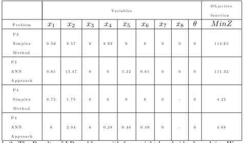
V a r i a b l e s O b j e c t i v e f u n c t i o n P r o b l e m x1 x2 x3 x4 x5 x6 x7 x8 M inZ P 3 S i m p l e x M e t h o d 0 . 5 0 8 . 5 7 0 8 . 9 3 0 0 0 0 0 1 1 4 . 6 5 P 3 A N N A p p r o a c h 0 . 6 1 1 3 . 4 7 0 0 5 . 2 2 0 . 6 1 0 0 0 1 1 1 . 3 2 P 4 S i m p l e x M e t h o d 0 . 7 5 1 . 7 5 0 0 0 0 0 - 0 4 . 2 5 P 4 A N N A p p r o a c h 0 2 . 0 4 0 0 . 2 8 0 . 4 0 0 . 4 0 0 - 0 4 . 0 8
Table 2. The Results of LP problems with fuzzy right hand sides by solving Werner’s approach
For the problems P3 and P4, simplex method and ANN approach are used. These problems are transformed to classical LP problems. The resulting LP problems are solved and obtained results have been given in Table 2. According to Table 2; as a result of solution to problem P3 and P4, it is seen that the method which gives minimum value to the objective function is ANN approach.
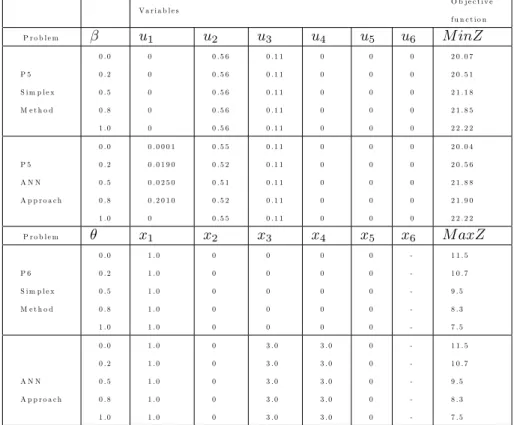
V a r i a b l e s O b j e c t i v e f u n c t i o n P r o b l e m u1 u2 u3 u4 u5 u6 M inZ P 5 S i m p l e x M e t h o d 0 . 0 0 . 2 0 . 5 0 . 8 1 . 0 0 0 0 0 0 0 . 5 6 0 . 5 6 0 . 5 6 0 . 5 6 0 . 5 6 0 . 1 1 0 . 1 1 0 . 1 1 0 . 1 1 0 . 1 1 0 0 0 0 0 0 0 0 0 0 0 0 0 0 0 2 0 . 0 7 2 0 . 5 1 2 1 . 1 8 2 1 . 8 5 2 2 . 2 2 P 5 A N N A p p r o a c h 0 . 0 0 . 2 0 . 5 0 . 8 1 . 0 0 . 0 0 0 1 0 . 0 1 9 0 0 . 0 2 5 0 0 . 2 0 1 0 0 0 . 5 5 0 . 5 2 0 . 5 1 0 . 5 2 0 . 5 5 0 . 1 1 0 . 1 1 0 . 1 1 0 . 1 1 0 . 1 1 0 0 0 0 0 0 0 0 0 0 0 0 0 0 0 2 0 . 0 4 2 0 . 5 6 2 1 . 8 8 2 1 . 9 0 2 2 . 2 2 P r o b l e m x1 x2 x3 x4 x5 x6 M axZ P 6 S i m p l e x M e t h o d 0 . 0 0 . 2 0 . 5 0 . 8 1 . 0 1 . 0 1 . 0 1 . 0 1 . 0 1 . 0 0 0 0 0 0 0 0 0 0 0 0 0 0 0 0 0 0 0 0 0 -1 -1 . 5 1 0 . 7 9 . 5 8 . 3 7 . 5 A N N A p p r o a c h 0 . 0 0 . 2 0 . 5 0 . 8 1 . 0 1 . 0 1 . 0 1 . 0 1 . 0 1 . 0 0 0 0 0 0 3 . 0 3 . 0 3 . 0 3 . 0 3 . 0 3 . 0 3 . 0 3 . 0 3 . 0 3 . 0 0 0 0 0 0 -1 -1 . 5 1 0 . 7 9 . 5 8 . 3 7 . 5
Table 3. The results of LP problems with fuzzy objective function parameter
For the problems P5 and P6, Simplex method and ANN approach are used. These problems are transformed to classical LP problems. The resulting LP problems are solved for di¤erent values and obtained results have been given in Table 3 According to Table 3; as a result of solution to problem P5, it is seen that, the method which gives minimum value to objective function is ANN approach for =0 and Simplex Method for =0.2, 0.5, 0.8, also for =1 the objective functions have equal values for simplex method and ANN approach. As a result of solution to problem P6, it is seen that objective function values reach the same value by using both of these methods.
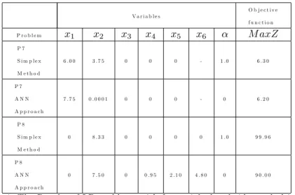
V a r i a b l e s O b j e c t i v e f u n c t i o n P r o b l e m x1 x2 x3 x4 x5 x6 M axZ P 7 S i m p l e x M e t h o d 6 . 0 0 3 . 7 5 0 0 0 - 1 . 0 6 . 3 0 P 7 A N N A p p r o a c h 7 . 7 5 0 . 0 0 0 1 0 0 0 - 0 6 . 2 0 P 8 S i m p l e x M e t h o d 0 8 . 3 3 0 0 0 0 1 . 0 9 9 . 9 6 P 8 A N N A p p r o a c h 0 7 . 5 0 0 0 . 9 5 2 . 1 0 4 . 8 0 0 9 0 . 0 0
Table 4. The Results of LP problems with fuzzy right hand sides and objective function
For the problems P7 and P8, simplex method and ANN approach are used. These problems are transformed to classical LP problems. The resulting LP problems are solved for di¤erent values and obtained results have been given in Table 4. According to Table 4, as a result of solution to problems P7 and P8, it is seen that the method which gives maximum value to the objective function is Simplex method. V a r i a b l e s O b j e c t i v e f u n c t i o n P r o b l e m x1 x2 x3 x4 x5 x6 x7 x8 M axZ P 9 S i m p l e x M e t h o d 1 . 2 2 7 3 . 8 1 8 0 0 0 0 0 0 2 1 . 4 0 9 P 9 A N N A p p r o a c h 1 . 2 2 7 3 . 8 1 8 0 0 . 3 2 7 0 . 9 0 0 0 . 0 4 1 0 . 2 9 5 0 2 1 . 4 0 9 P 1 0 S i m p l e x M e t h o d 0 0 0 0 0 0 - - 5 0 . 0 0 P 1 0 A N N A p p r o a c h 0 . 0 3 0 1 . 0 4 0 0 0 . 0 4 1 - - 5 2 . 8 2
Table 5. The Results of LP problems with fuzzy right hand sides and coe¢ cient matrix
For the problems P9 and P10, simplex method and ANN approach are used. These problems are transformed to classical LP problems. The resulting LP
problems are solved and obtained results have been given in Table 5. According to Table 5; as a result of solution to problem P9, it is seen that objective function reaches the same value by using both of these methods. Also, as a result of solution to problem P10, it is seen that the method which gives maximum value to the objective function is ANN approach.
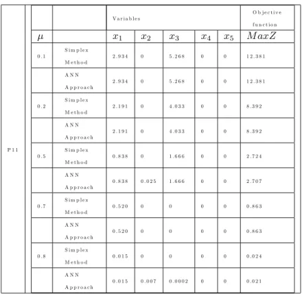
P 1 1 V a r i a b l e s O b j e c t i v e f u n c t i o n x1 x2 x3 x4 x5 M axZ 0 . 1 S i m p l e x M e t h o d 2 . 9 3 4 0 5 . 2 6 8 0 0 1 2 . 3 8 1 A N N A p p r o a c h 2 . 9 3 4 0 5 . 2 6 8 0 0 1 2 . 3 8 1 0 . 2 S i m p l e x M e t h o d 2 . 1 9 1 0 4 . 0 3 3 0 0 8 . 3 9 2 A N N A p p r o a c h 2 . 1 9 1 0 4 . 0 3 3 0 0 8 . 3 9 2 0 . 5 S i m p l e x M e t h o d 0 . 8 3 8 0 1 . 6 6 6 0 0 2 . 7 2 4 A N N A p p r o a c h 0 . 8 3 8 0 . 0 2 5 1 . 6 6 6 0 0 2 . 7 0 7 0 . 7 S i m p l e x M e t h o d 0 . 5 2 0 0 0 0 0 0 . 8 6 3 A N N A p p r o a c h 0 . 5 2 0 0 0 0 0 0 . 8 6 3 0 . 8 S i m p l e x M e t h o d 0 . 0 1 5 0 0 0 0 0 . 0 2 4 A N N A p p r o a c h 0 . 0 1 5 0 . 0 0 7 0 . 0 0 0 2 0 0 0 . 0 2 1
Table 6. The Results of LP problems with all fuzzy coe¢ cient
Problem P11 is transformed to classical LP problems. This problem is solved by both Simplex method and ANN approach for di¤erent values. The resulting LP problems are solved and obtained results have been given in Table 6. Ac-coding to Table 6; for =0.1; 0.2 and 0.7 it is seen that the results from both of two methods are the same. Also it is concluded that the results for =0.5 and 0.8 are di¤erent and maximum objective function value is obtained by Simplex method.
5. Result
In this study, uncertainty in the right hand sides, objective function parameters, right hand sides and objective function, right hand sides and coe¢ cient matrix
and all coe¢ cients are considered for FLP. For envisaged …ve di¤erent struc-ture, FLP problems are solved by using Simplex method and ANN approach. Interpretations connected with obtained solutions are given in tables seperately. Investigating all results, two main interpretations can be explained.
First, the ANN approach is better than simplex method for the results of LP model with fuzzy right hand sides, LP model with fuzzy objective function parameter, LP model with fuzzy right hand side(s) and coe¢ cient matrix, LP model with all fuzzy coe¢ cient objective function parameter. For example; from Table 1. it is obviously seen that, in the problem P2 with =1 that is one of the LP problem with fuzzy right hand sides by solving Verdegay’s approach, the value of MinZ is 11.5 for both ANN approach and Simplex Method. From Table 2, in the problem P3 that is one of the LP problem with fuzzy right hand sides by solving Werner’s approach, the value of MinZ is 4.08 for ANN Approach and the value of MinZ is 4.25 for Simplex Method. From Table 3, in problem P5 with =0 that is one of the LP problem with fuzzy objective function parameter, the value of MinZ is 20.04 for ANN Approach and the value of MinZ is 20.07 for Simplex Method. From Table 5, in problem P10 that is one of the LP with fuzzy right hand sides and coe¢ cient matrix, the value of MaxZ is 52.82 for ANN Approach and the value of MaxZ is 50.00 for Simplex Method. From Table 6, in problem P11 with =0.2 that is one of the LP with all fuzzy coe¢ cient, the value of MaxZ is 8.392 for both ANN approach and Simplex Method.
Second, by using ANN approach, more variables have positive value than sim-plex method. For example; in problem P1 with =1, eight(8) variables have positive value for ANN Approach and two(2) variables have positive value for Simplex Method.
We have shown that, the ANN approach are very useful and appliciable for FLP models. Consequently, the ANN approach can be an alternative to the other methods such as Simplex method for the solution of FLP models.
6. Appendix P1: M ax Z = x1+ 2x2 3x1+ 3x26 ~9 x1 x26 2 x1+ x26 ~6 x1+ 3x26 ~6 xj> 0; j = 1; 2
For the problem P1, tolerances of the …rst, the third and the fourth right hand sides are given p1= 3; p3= 3 and p4= 1 respectively (Arti…cial data).
P2: M in Z = 5x1+ 2x2 4x1+ x26 ~8 x1+ x26 ~5 x26 ~2 x16 ~0 xj > 0; j = 1; 2
For the problem P2, tolerances of the …rst, the second, the third and the fourth right hand sides are given p1= 3; p2= 1; p3= 2 and p4= 1 respectively
(Arti…cial data). P3: M in Z = 4x1+ 5x2+ 9x3+ 11x4 x1+ x2+ x3+ x46 1~5 7x1+ 5x2+ 3x3+ 2x46 8~0 3x1+ 5x2+ 10x3+ 15x46 1~00 xj > 0; 2 [0; 1]; j = 1; 2; :::; 4
For the problem P3, tolerances of the …rst, the second and the third right hand sides are given p1= 5; p2= 40 and p3= 30 respectively [6].
P4: M in Z = x1+ 2x2 3x1+ 3x26 ~9 x1 x26 2 x1+ x26 ~6 x1+ 3x26 ~6 xj > 0; j = 1; 2
For the problem P4, tolerances of the …rst, the third and the fourth right hand sides are given p1= 3; p3= 1 and p4= 1 respectively (Arti…cial data).
P5:
M ax Z = 2~1x1+ 2~7x2+ 4~5x3+ 3~0x4
x1+ x2+ 4x3+ 3x4> 1
3x1+ 3x2+ 3x3+ x4> 1
xj > 0; j = 1; 2; 3; 4
For the problem P5, …rst the dual form of P5 is obtained. Then, the …rst, the second, the third and the fourth right hand sides are given p1= 3; p2= 3; p3=
5 and p4= 4 respectively (Arti…cial data).
M ax Z = ~6x1+ ~3x2
2x1> 1
x1+ 2x2> 2
x1 x2> 1
x1; x2> 0
For the problem P6, …rst the dual form of P6 is obtained. Then, the …rst and the second right hand sides are given p1= 2 and p2= 1 respectively (Arti…cial
data). P7: M a~x Z = 80x1+ 40x2> 630 x16 ~6 x26 ~4 xj > 0; j = 1; 2
For the problem P7, objective function value and its tolerance are given as bG = 630 and pG = 10. Tolerance of right hand sides are given p1 = 1 and
p2= 2 respectively (Arti…cial data).
P8: M a~x Z = 6x1+ 12x2 6x + 3x2> 1~8 2x1+ 4x2> 1~2 2x1+ 8x2> 1~6 xj > 0; j = 1; 2
For the problem P8, objective function value and its tolerance are given as bG = 100 and pG = 10. Tolerance of right hand sides are given p1= 5; p2 = 3
and p3= 4 respectively (Arti…cial data).
P9:
M ax Z = 5x1+ 4x2
h4; 2; 1i x1+ h5; 3; 1i x26 h24; 5; 8i
h4; 1; 2i x1+ h1; 0:5; 1i x26 h12; 6; 3i
x1; x2> 0
For the problem P9, fuzzy numbers are expressed by ha; l; ri and hb; u; vi. Then multiplication and summation operations are used for these fuzzy numbers [5]. P10:
M ax Z = 20x1+ 30x2+ 50x3
h6; 2; 10i x1+ h5; 1; 8i x2+ h7; 3; 10i x36 h8; 4; 15i
For the problem P10, fuzzy numbers are expressed by ha; l; ri and hb; u; vi. Then multiplication and summation operations are used for these fuzzy numbers (Arti…cial data). P11: M ax Z = (2; 1]x1+ (0:5; 1:5]x2+ (0:8; 1:2]x3 (3; 5]x1+ (1:5; 2:5]x2+ (0; 3]x36 (8; 12] (0:5; 1:5]x1+ (1:8; 3:8]x2+ (1; 3]x36 (6; 9] xj > 0; j = 1; 2; 3
In the problem P11, all coe¢ cients are fuzzy. The constants –0.3 and 2 is determined by decision maker indicate that a pozitive number implies convex exponential function and a negative number implies concave exponential func-tion. Thus, the original fuzzy linear programming with absolute trade-o¤ is equivalent to following problem.
References
1. Carlsson, C. And Korhonen, P. (1986), A Parametric Approach To Fuzzy Linear Programming. Fuzzy Sets And Systems 20, 17-30.
2. Chanas, S. (1983), The Use Of Parametric Programming In Fuzzy Linear Program-ming. Fuzzy Sets And Systems 11, 243-251.
3. Delgado, M., Verdegay, J.L. And V¬la, M.A. (1989), A Genaral Model For Fuzzy Linear Programming. Fuzzy Sets And Systems 29, 21-29.
4. Haykin, S. (1994), Neural Networks: A Comprehsive Foundation, Macmillan, New York.
5. Klir, G.J. And Yuan, B. (1995), Fuzzy Sets And Fuzzy Logic: Theory And Appli-cation, Prentice Hall P T R, New Jersey.
6. Lai, Y. And Hwang, C. (1992), Fuzzy Mathematical Programming, Sringer-Verlag, Berlin Heidelberg.
7. Patterson, D.W. (1996), Arti…cal Neural Networks:Theory And Applications, Pren-tice Hall, New York.
8:Sugeno, S. And S¬ganos, D. (1996), Neural Networks. Web Page Address:Http://Www-Dse.Doc.·Ic.Ac.Uk/~Nd/ Surprise_96/Journal/V.../Report.Htm
9. Sungur, M. (1995) Mühendis Gözüyle Yapay Sinir A¼glar¬, O.D.T.Ü, Ankara. 10. Terano, T. , Asa¬, K.And Sugeno, M. (1981), Fuzzy Systems Theory And It’s Applications, Academic Pres Inc, San Diego.
11. Vemur¬, R.V. (1992), Arti…cial Neural Networks: Concepts And Control Applica-tions, Ieee Computer Society Press, Los Alamitos, California.
12. Wang, J. And Chankong, V. (1992), Recurrent Neural Networks For Linear Pro-gramming: Analysis And Design Principles. Computers Ops. Res. 19 (3/4), 297-311.
13. Wassermann, P.D. (1989) Neural Computing: Theory And Practice, Von Nostrand Reinhold, New York.
14. Yap¬c¬, N. (2000), Bulan¬k Do¼grusal Programlamaya Sinir A¼glar¬Yakla¸s¬m¬, Yük-sek Lisans Tezi (Bas¬lmam¬¸s), Fen Bilimleri Enstitüsü, Konya.
15. Zadeh, L.A. (1965), Fuzzy Sets, Information And Control, 8,338-353.
16. Zimmermann, H.J. (1983), Fuzzy Mathematical Programming. Computers Ops. Res. 10 (4), 291-298.