https://doi.org/10.1177/0020294018758527 Measurement and Control 2018, Vol. 51(1-2) 38 –56 © The Author(s) 2018 Reprints and permissions:
sagepub.co.uk/journalsPermissions.nav DOI: 10.1177/0020294018758527 journals.sagepub.com/home/mac
Creative Commons CC BY: This article is distributed under the terms of the Creative Commons Attribution 4.0 License (http://www.creativecommons.org/licenses/by/4.0/) which permits any use, reproduction and distribution of
the work without further permission provided the original work is attributed as specified on the SAGE and Open Access pages (https://us.sagepub.com/en-us/nam/open-access-at-sage).
I. Introduction
Mobile robot applications are growing in significance in research and daily-life implementations. These robots are commonly used in a wide range of fields and applications such as in industrial plants, commercial zones, medical sys-tems, material handling, and the defense industry. The major advantage and superiority of mobile robots over leg-ged counterparts are design and control simplicity, reduced manufacturing and maintenance costs, and longevity. The legged-robots are also capable of tackling obstacles and uneven terrain difficulties.1 However, it is a tedious task to
maintain the control of a legged-robot due to the complex-ity of its structure.2 Mobile robots can be mainly configured
as three-, four-, and six-wheel structures, which are stati-cally stable systems for ease of control and energy effi-ciency. Among these the most popular one is the four-wheel structure, ensuring stability at high speeds and under cer-tain disturbances. On the other hand, due to the physical characteristics of four wheels, it is dependent on suspen-sion systems to keep the wheels in contact with the road.
Besides these configurations, there are also two-wheeled mobile robots available. Two-wheeled mobile robots are basically called “two-wheeled balancing robots” (TWBR) due to their unstable dynamical characteristics. Although controlling two-wheeled robots is a challenging issue, they can be regarded as simpler structured mechanisms than leg-ged-robots. Their advantages over other configurations are high maneuverability capabilities, small footprints, and ability to turn around their own axis, but they can be less
power efficient due to the continuous need to balance. However, thanks to this continuous dynamical stabilization, the robot can reject disturbances affecting the body and can have a wider range of center of gravity (COG) variance. This lets the designer place additional payloads and struc-tures on the system.3 The most common structure of the
TWBR is two electrical-motor-powered wheels connected to the main stationary body. The stationary part of the robot is essentially an inverted pendulum whose stability must be achieved with the effort of the two actuated wheels.4
Due to structural advantages and being a challenging control problem, TWBR is an important problem attracting interest in numerous research and application works.4,5–9
Linear controllers such as proportional integral derivative (PID) and linear quadratic Gaussian (LQR) can be designed and comprehended easier than complex nonlinear and adaptive ones.10 For this purpose, a linear dynamical model
of the system is derived around predefined equilibrium points. For a given linearized model, it is straightforward to apply established methods such as pole placement11 and
LQR12,13 to maintain the stability of the system. Various
studies also show comparisons among different linear con-trol schemes.14,15 The performance of the linear controllers
Adaptive Model Predictive
Control of a Two-wheeled Robot
Manipulator with Varying Mass
Mert Önkol and Coşku Kasnakoğlu
Abstract
This paper presents the adaptive model predictive control approach for a two-wheeled robot manipulator with varying mass. The mass variation corresponds to the robot picking and placing objects or loads from one place to another. A linear parameter varying model of the system is derived consisting of local linear models of the system at different values of the varying parameter. An adaptive model predictive control controller is designed to control the fast-varying center of gravity angle in the inner loop. The reference for the inner loop is generated by a slower outer loop controlling the linear position using a linear quadratic Gaussian regulator. This adaptive model predictive control/linear quadratic Gaussian control system is simulated on the nonlinear model of the robot, and the closed-loop performance of the proposed scheme is compared with a system having inner/outer loop controllers as proportional integral derivative/ proportional integral derivative, feedback linearization/linear quadratic Gaussian, and linear quadratic Gaussian/linear quadratic Gaussian. It is seen that adaptive model predictive control shows mostly superior and otherwise very good performance when compared to these benchmarks in terms of reference tracking and robustness to mass parameter variations.
TOBB University of Economics and Technology, Ankara, Turkey
Corresponding author:
Coşku Kasnakoğlu, TOBB Ekonomi ve Teknoloji Universitesi, Sogutozu Cd. No. 43, Ankara, 06560, Turkey.
Email: [email protected]
is dependent on the selection of the control parameters such as Q 1 0 0 1
and R.16 This can be thought of as a tradeoff
between fast response and robustness. One also finds appli-cations of LQG control, which combines Kalman filtering with LQR.17 These have also been adapted to linear
time-varying systems for reference trajectory tracking.18
2
design has also been investigated and compared to simpler designs (e.g. LQR), where it was seen that the former sus-tains stability and performance over longer time durations.19
Despite the availability of advanced methods, simple PID designs still dominate industrial applications due to their simple structure and ease of tuning.20,21 Since PID
controllers are essentially single-input single-output in nature, multiple controllers must be designed for the tilt angle and position of the vehicle.22 These two modes must
also be assumed to be decoupled, which may prove to be incorrect if the departure from the operating point is large. Employing nonlinear control techniques could remedy this drawback allowing the designer to work on a wider scale of operating conditions.23,24 For instance, the combination of
PID and backstepping controllers are presented and the advantages of each method are depicted in Lee et al.25
Sliding mode control (SMC) is also possible, a method known for its powerful capabilities and robustness against system uncertainties and perturbations.26 SMC drives the
system to a predefined hypersurface and ensures exponen-tial convergence to origin, while rejecting disturbances and perturbations.27 Another possibility is feedback
lineariza-tion (FBL; i.e. dynamic inversion), where the system non-linearities are cancelled through feedback, after which the problem reduces to linear control.28,29 Numerous other
non-linear control approaches were tested on TWBR systems, including fuzzy PID with satisfactory results.30
Adaptive control strategies are methods applicable to time-varying and uncertain systems for maintaining perfor-mance criteria and stability. Myriad studies are available varying from simple double integrator systems to complex
chemical processes.31 Different adaptive control strategies
were successfully implemented on TWBR as well. In Degani et al.,32 the center of mass height was tracked by
checking the deviation from the COG and the system was kept stable with adaptive control techniques. Adaptive and fuzzy controllers were merged for real-time adjustment of the membership functions in Wang et al.33 Other examples
include neural-adaptive output feedback control of trans-portation vehicles based on wheeled inverted pendulum models34 and two-timescale-tracking control of
nonholo-nomic wheeled mobile robots.35
Model predictive control (MPC) strategy is widely used in the process control industry, especially for systems with slow dynamics. The MPC performance depends on the dynamical model of the process or system. MPC takes the current time into account, sustaining optimality while keep-ing incomkeep-ing future timeslots. This is an iterative and finite time horizon optimization method. MPC achieves predic-tion of the future states of the linear time-invariant (LTI) model of the nonlinear plant linearized around specific equilibrium points. Practically, the prediction of MPC is sensitive to prediction errors. This is acceptable for lowly nonlinear systems. On the other hand, TWBR includes highly coupled nonlinear dynamics, limiting the ability of MPC control to achieve satisfactory performance and sta-bility. To resolve this problem, adaptive model predictive control (AMPC) can be employed.36 AMPC can handle
per-formance degradation of the MPC controller due to the strong nonlinearity. AMPC uses changing operating points to update the prediction model. The advantage of using AMPC is the convenience of constructing on a predesigned MPC structure. Studies on the AMPC control scheme applied to different systems are becoming more appealing as computing capabilities increase.37,38
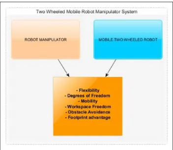
In this study, we investigate combining a TWBR base with a robot manipulator, in particular controlling its posi-tion. This generates a type of robotic system valuable for industrial and daily-life applications. A robot manipulator consists of one or more rigid links connected via fixed or actuated joints. Robot manipulators are useful for picking/ placing objects, assembly, and applications hazardous/ inappropriate for humans. Their disadvantage is limited workspace due to a fixed base point. Integrating with a TWBR could thus remedy this drawback, achieving high mobility and maneuverability in diverse environments.39,40
The benefits of such integration are summarized in Figure
1. The aim of this study is to prove the usefulness of AMPC
for such an integrated robot, in the sense that desired track-ing performance outperforms various standard control approaches. Our method builds upon a new linear parame-ter varying (LPV) modeling approach,41–45 so that mass
variations corresponding to the robot manipulator’s actions are captured. Typical robot manipulators are actuated sys-tems since the number of degrees of freedom and actuators are equal. After merging a TWBR with a robot manipulator the system becomes underactuated, and from the control-ler’s perspective it is similar to an inverted pendulum on a cart.46 In this study the setup investigated consists of four
manipulator links, which are considered as one virtual link.
The use of this equivalence allows simpler dynamical mod-eling. The control goal is to robustly track position while coping with this underactuated structure, nonlinear dynam-ics, and disturbances from various sources.
The rest of this paper is organized as follows: Mathematical modeling of system is presented first, deriv-ing the equivalent inverted pendulum representation. Once the model is obtained, various control approaches are developed, consisting of an inner loop for the faster angle dynamics, and an outer loop for the slower linear position. These approaches considered are PID/PID, LQG/LQG, FBL/LQG, and finally AMPC/LQG, where the X/Y nota-tion denotes X for inner controller and Y for outer control-ler. Simulations are carried out for all, where a reference trajectory is tracked in the presence of mass variations. The results are evaluated in terms of various metrics. The paper ends with conclusions and future directions.
II. Mathematical Modeling
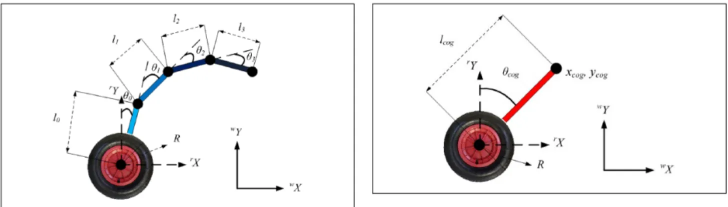
In order to design and implement controllers, an appropriate model of the proposed system was created under MATLAB/ Simulink numerical computing environment. During the modeling phase, different toolboxes were employed such as SimMechanics and control systems. The system configura-tion is based on the study of Chen et al.,39 which is
illus-trated in Figure 2. The manipulator consists of four links as seen in the figure. The first link, that is, the link connected to the wheel, is passive while the others are actuated.
The parameters of the robot are as follows: R is the radius of wheels, rX, rY is the robot coordinate frame, wX, wY is the world coordinate frame, xcog, ycog is the position of the COG, l0 is length of the passive joint, l1,2,3 are the lengths of
links 1, 2, 3 respectively, θ0 is the angle between the wheels
and passive joint, and θ1,2,3 are the angles between an active
link and its predecessor link.
The governing equations describing the motion of the mobile robot manipulator are
τ=Μ ( )θ θ+H( , )θ θ θ +g( )θ (1) where τ = [τw, 0, τ1, τ2, τ3] is the input torque, θ = [θw, θ0, θ1,
θ2, θ3] is the vector of angles, and M, H, q(θ) are,
respec-tively, the inertia, centrifugal force, Coriolis force, and gravity matrices. Due to the complex structure of the robot manipulator, system modeling requires many equations to describe the entire system. Having four links is useful in terms of extended physical capabilities, but increases model complexity. In order to simplify modeling, the system could be considered as a single rod virtual inverted pendulum as shown in Figure 3. As depicted in the model, mass and inclination of four links are represented by a virtual link mass at the COG and its angle with the wheel. These can be computed with the following mathematical calculations
x m x m y m y m x cog i i i i i cog i i i i i cog cog = ∑ ∑ = ∑ ∑ = = = = = 0 3 0 3 0 3 0 3 , arctan θ yycog cog i i cog m m l xcog ycog = ∑ = + = , , 0 3 2 2 (2)
At this point Euler-Lagrange method can be employed for derivation of the dynamical model of the inverted pen-dulum. The dynamical equation of motion of entire system can be written as follows
τ=Μ ( )θ θ+H( , )θ θ θ +g( )θ (3)
where θ θ θ=[ ,w cog] and τ τ=[ , ]w 0 are coordinate and input torque vectors. From here, the derived systems dynamics are as follows
Figure 3. Virtual inverted pendulum model. Figure 2. Mobile manipulator model.
d
dt L L
mlcog ml
w w w w
w cog cog cog
∂ ∂ − ∂∂ = → = + − θ θ τ θ
τ θ cosθ θ2sinθccog
cog cog cog w cog cog
M m d dt L L g ( ) cos sin + ∂ ∂θ − ∂∂θ =0 → θ =θ θ + θ (4)
where M is the mass of the mobile part and m is the mass of COG, respectively.
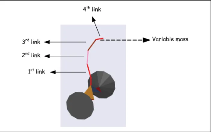
An important aspect of this research is to have a variable mass on the robot to carry out various tasks. While han-dling different tasks, the system acts like a time-variant sys-tem as the mass of entire body changes at the time frame of working, for instance, when the robot picks a load from a point and drops off in a different location. If the system is not designed with robustness enough to handle the effect of mass variance, stability and reference tracking may not be sustained, causing violent oscillations or instability. To compare the difference, the robot is modeled under two conditions, namely, with variance in mass and without
variance in mass. Pick and place scenarios were applied in the simulation studies. Figure 4 shows the three-dimen-sional (3D) model of the manipulator realized in SimMechanics.
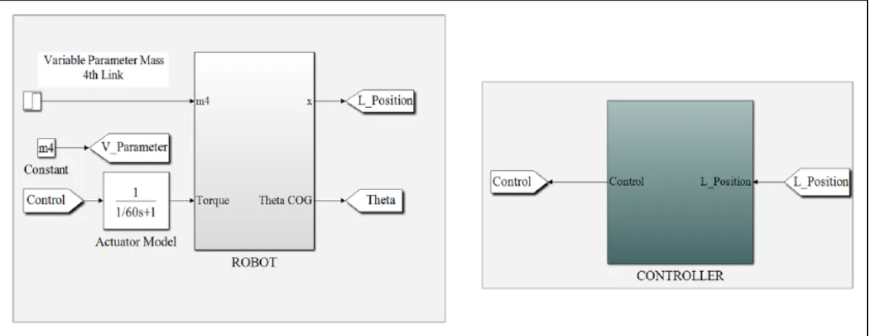
The Simulink block diagram is given in Figure 5 and the key parameters of the system are depicted in Table 1. In the block diagram, the joint between the first link and the main body is unactuated while the other joints are actuated by the controller. Unlike the other links, the last link was modeled adding variable a mass input to the arm representing pick-ing up or puttpick-ing down objects. This mass variance effect is a key consideration in mathematical modeling and control-ler design.
III. Control Design
Due to its statically unstable structure, a dynamic controller is required to maintain stability of the balancing robot. The ultimate objective in control is balancing the COG of the virtual link, whose position, angle, and mass will change based on the task carried out by the manipulator. Thus, a robust control system to suppress the adverse effects of the disturbances, perturbations, unmeasured dynamics, and variable mass is needed to handle the control task. The robot system is underactuated from the perspective of con-trolling the COG; only the wheels provide the control (see
Figure 5). There are, however, 2 degrees of freedom,
namely, the location of the COG and the linear position of
Figure 4. Variable mass scenario.
the robot, which have coupled dynamics between each other. The challenge is therefore to control a coupled dynamics with only one input.
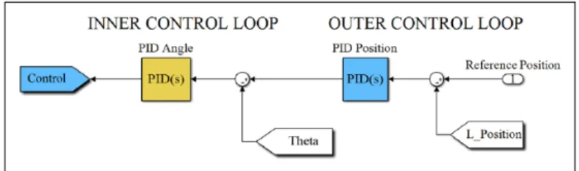
The control systems literature offers a wide range of solutions when it comes to controlling underactuated dynamical systems. The dynamics of the mobile robot manipulator are such that the 2 degrees of freedom can be categorized as fast and slow dynamics. The fast dynamics are those related to the inner loop of the vehicle, that is, the angle of the link. The slow dynamics are those related to the outer loop of the vehicle, that is, the linear position of the wheels. In control design the major emphasis is placed on stabilization of fast dynamics, which plays a significant role in the behavior of the vehicle as a whole. The slow dynamics, that is, linear position, is then controlled as an outer loop by manipulating the angle inside the inner loop (Figure 6). Various control design methods are imple-mented in the succeeding sections and are compared in terms of the metrics integral absolute error (IAE), mean absolute error (MAE), integral squared error (ISE), and integral squared control input (ISCI).
IV. Proportional Integral Derivative
Control Scheme
PID control is one of the earliest yet most popular control schemes due to the ability to perform easy empirical tuning for satisfactory performance.40 To design the PID
control-ler, nonlinear dynamics of the vehicle are first linearized around the zero equilibrium point (i.e. when the robot is stationary in an upright position). Then dynamics of rota-tional behavior (COG angle) are control by tuning the coef-ficients of the inner PID controller until satisfactory
performance. Next, for controlling the linear position the coefficients of the outer loop PID are adjusted, fixing the inner PID controller. The process is iterated a number of times until the angle and position responses are as desired. Further fine-tuning is performed to account for the effects caused by mass variations. The ultimate values of the inner loop coefficients are Kp1 = −77.306, Ki1 = −8.721, and
Kd1 = −28.862 and those of the outer loop are Kp2 = 0.426,
Ki2 = 0.02, and Kd2 = 1.319. It is expected that larger control coefficients are required for the inner loop PID controller because tracking and stabilizing of the fast dynamics need more aggressive control effort. The block diagram imple-mentation of the control system can be seen in Figure 7. For realistic simulations, measurement noise is also added to the angle and position inputs of the control.
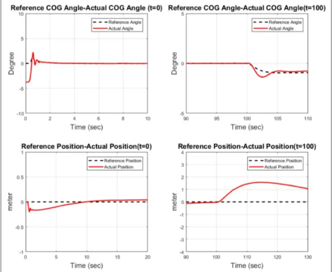
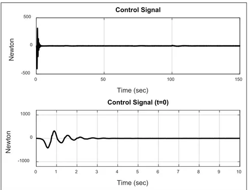
The results of the PID control approach can be observed in Figures 8–10. According to the simulation scenario, mass of the last link, that is, link 4, is changed from 0.2 to 0.4 kg at t = 100 s in order to test the robustness of the con-trolled plant against variances in mass. The initial condi-tions for the links are, respectively, −10, 10, 10, and 10°. The angular control loop exhibits sufficient performance and the position controller shows good tracking perfor-mance until 100 s. With the change of mass of the last link at time t = 100 s, the position controller performance severely deteriorates and takes a significant time to settle. The performance metrics for the PID controller are tabu-lated in Table 2.
V. Linear Quadratic Gaussian
Control
LQG is a dynamical controller for the system written in the form x Ax B w y Cx Du v
u
= + + = + + (5)where x is state vector, u is plant input, y is the plant output,
w is the process noise representing modeling errors, and v is
the output noise representing measurement errors. A, B, C, D
Table 1. Parameters of the system.
Mass of mobile robot (M) 18 kg
Lengths of the links (m0, m1, m2, m3) 1.5, 0.7, 0.4, 0.2 kg
Masses of the links (l0, l1, l2, l3) 0.2, 0.2, 0.2, 0.1 m
Radius of the wheels (R) 0.15 m Width of the mobile body (W) 0.65 m
are the state-space matrices. LQG is in fact a combination of the linear quadratic regulator (LQR), an optimal controller, and the Kalman filter, an optimal estimator. The objective of the LQR controller is to minimize the cost function J
J E= →∞
∫
x Q x u Ru x Q x dtT + T + iT i i lim τ τ τ10 (6)where E denotes the expected value, xi is integral of the reference tracking error of the output signal, and Q, R, Qi are, respectively, weighing matrices for states, input, and integral error. Due to the lack of measurements from all states of the system, a Kalman filter is employed which
provides optimal estimates for x (denoted xe) by minimiz-ing the function
P E x x x x t e e T = − − →∞
{
}
lim ( )( ) (7)given the process and measurement noise covariances Qn and Rn. During the design phase of the LQG controller, the system is again linearized around the zero equilibrium point and the design is carried out by selecting the param-eters as in Table 3. The results for the LQG controller sys-tem can be seen in Figures 11–13. The figures correspond to the COG angle, linear position tracking, variable mass change, and control effort, respectively. It can be observed
Figure 7. Cascaded PID control structure.
Figure 9. Transient and parameter change responses.
from the figures that both the LQG controllers are capable of following and suppressing the effect of the changing mass at t = 100 s. After some fluctuation the system settles down to steady state within about 20 s. The performance metrics for LQG are shown in Table 4. It is seen that the ISCI index is lower than PID, that is, less control effort is required. All the error metrics (IAE, MAE, ISE) are also lower, meaning that the LQG controller has better reference tracking and robustness to parameter variations.
VI. Feedback Linearization Control
FBL (also called dynamic inversion) is a nonlinear control approach that can produce exact linear representation of the
plant model. FBL employs transformation of the nonlinear system into equivalent linear system by applying appropri-ate control input (Kim et al., 2010).47 Since no
approxima-tion is made (in contrast to approximate Jacobian linearization), FBL is valid over the entire operating enve-lope and not just within a local neighborhood.
Let the dynamics of a nonlinear system be expressed as
x( )n =Sf bu+ (8)
where f = ( ) and b b xf x = ( ) are dependent on the states.
The goal is to utilize a control input
u b= −1(− +f v) (9)
Table 2. Performance measures for PID control scheme.
Criterion Position (x) Center of mass angle (θcog) Control input (U)
IAE 70.5 6.533 –
MAE 0.01367 0.0287 –
ISE 64.73 7.444 –
ISCI – – 8.137 × 10⁵
IAE: integral absolute error; MAE: mean absolute error; ISE: integral squared error; ISCI: integral squared control input.
Figure 12. Transient and parameter change responses.
so as to make the system exactly linear as
x( )n =v (10)
after which v can be designed using linear control theory. For our system, the fast dynamics that control the angle of the robot have significant importance on the overall perfor-mance, so we shall focus on that part
m lcog cog2θcog=mcogglcogsin(θcog)−u (11)
where u is input torque to the wheels. This can be arranged as
θcog θ
cog cog cog
g
l ml u
= sin( )− 12 (12)
which is of the form of equation (8). Utilizing an FBL con-troller of the form of equation (9)
u m l g l v cogcog cog cog = − − + 2 sin(θ ) (13) yields θcog v= (14) Let v=θcogd−αe ke− (15)
where e=θcog−θcogd is the tracking error, θcogd is the reference angle, and α,k are the design parameters. Substituting into equation (14) results in the tracking error dynamics
e+αe ke+ =0 (16)
which is asymptotically stable for α,k > 0, achieving
e→ 0 and thus the desired tracking. Combining equations (13) and (15) gives controller explicitly as
u m lcogcog lg e ke
cog cog cogd
= − − + − − 2 sin(θ ) θ α (17)
which completes the inner loop controller design via FBL. For the outer loop we utilize LQG to control the position, making this an FLB/LQG controller overall. After numerous iterations the controller parameters giv-ing the best results are given in Tables 5 and 6. The simu-lation results with these parameters are plotted in Figures
14–16. The controller starts out acceptably, albeit with
some oscillations. The mass change at t = 100 s, how-ever, degrades tracking considerably, which takes quite a while to settle back. The performance metrics are given in Table 7. It is seen that the tracking performance is quite inferior to LQG. The control effort is somewhat lower, but this is of little value in presence of the degraded performance. Also, no clear advantage is obtained over PID as some metrics are higher, while some are lower.
VII. Adaptive MPC Control
Model predictive control (MPC) is a method for process control that actively uses the dynamical model of the sys-tem. The system is optimized within a predefined time slot in which MPC estimates the future states and controls of system. While this is quite computationally intensive, advances in digital computing have increased the feasibility of the MPC approach greatly. MPC can be implemented in the presence of uncertainties on linear and nonlinear sys-tems. If the nonlinearity is high, however, MPC perfor-mance could deteriorate. In this case, one can use an adaptive model predictive controller that constantly pre-dicts the new operating conditions. For instance, AMPC can be used on linear time-varying (LPV) systems with uncertainties, where the controller parameters are tuned in closed loop employing real-time measurements.41,46
The MPC algorithm solves a quadratic optimization prob-lem at each time interval. The solution of the probprob-lem deter-mines the so-called manipulated variables (MV), which are essentially the input variables adjusted dynamically to keep the controlled variables (CV) at their set-points. The AMPC approach follows the same cost optimization algorithm as MPC with the cost function
Table 4. Performance measures for LQG control scheme.
Criterion Position (x) Center of mass angle (θcog) Control input (U)
IAE 16.82 6.228 –
MAE 6.073 × 10⁻⁴ 1.584 × 10⁻⁴ –
ISE 10.65 3.351 –
ISCI – – 3.513 × 10⁴
IAE: integral absolute error; MAE: mean absolute error; ISE: integral squared error; ISCI: integral squared control input. Table 3. Parameters for LQG control scheme.
Parameter Inner loop controller Outer loop controller
Q 0.01 0.1
R 0.00001 0.1
Qi 0.8 0.8
Qn 1 × I5 0.1 × I13
Figure 14. FBL angular and LQG positional tracking with mass change.
J zy k w s r k i k y k i k i y y y j y j j i p j n ( ) , | | =
(
( + )− ( + ))
= = ∑ ∑ 1 1 2 (18)where k represents the current control interval, p is the predic-tion horizon (interval number), ny is the number of plant output variables, zk is the quadratic problem (QP) selection which is depicted as zkT =[ ( | ) u k k T u k( +1 | ) ... ( +k T u k p−1| ) ], kT k yj(k + i|k) is the jth CV at the ith prediction horizon step,
rj(k + i|k) is the ith references variable at the ith prediction horizon step, sjy is the scale factor for the jth plant output variable, and wi jj, is the tuning weight coefficient reflecting the relative importance of the plant output variable. Among these variables ny, syj, p, and wi jj, are determined during the controller design and stay constant. Let the prediction model be described as follows
Table 5. FBL controller parameters.
Feedback linearization controller
k 10
α 0.1
Table 6. LQG controller parameters.
Outer loop controller
Q 0.01
R 0.01
Qi 0.6
Qn 0.1 × I9
Rn 1
Figure 16. Control signal of FBL.
Table 7. Performance measures for FBL and LQG control schemes.
Criterion Position (x) Center of mass angle (θcog) Control input (U)
IAE 21.6 11.83 –
MAE 9.495 × 10⁻³ 2.436 × 10⁻⁴ –
ISE 12.18 4.432 –
ISCI – – 1.053 × 10⁴
IAE: integral absolute error; MAE: mean absolute error; ISE: integral squared error; ISCI: integral squared control input.
x A x B u B v B w y C x D v D w k k u k v k w k k k v k w k + = + + + = + + 1 (19)
where vk is the measurement noise and wk = [dk, ek] is the process noise. The future trajectories of the dynamical model are predicted over the prediction horizon Hp. Setting all wk = 0 for all prediction instances the equation becomes yk H kp C AHpxk H B uk j H i i j A p u p + = + − − + = = − ∑ ∑ | 1 0 0 1 1 ∆ + D vv H p (20)
The solution can be summarized for all the Hp predicted time intervals as follows
y y y S x S u S u u k k k H x k u k u k k p + + + − − + = + + 1 2 1 1 1 ∆ ∆ ∆∆u H v v k Hp v k k k H v p + − + + + 1 1 (21) where Sx CA CA CA S CB CAB CB CA B H H n n u u u u j p p y x = ∈ = + × − 2 1 R uu j H H n n u u u u p p x u S CB CB CAB CB = × − ∑ ∈ = + 0 1 0 0 R uu j u j Hp j u j Hp u H CA B CA B CB 0 0 1 0 1 = − = − ∑ ∑ ∈R pp yn H np u v v v v Hp v Hp v Hp H CB D CAB CB D CA B CA B CA × − − − = 0 1 2 3 B Bv D H np y Hp nv 0 0 1 ∈ × + R ( ) (22)
Regarding the equations mentioned above, the optimi-zation function can be introduced as
J z u u p u u p r r ( , ) ( ) ( ) ( ) ( ) ε = − − − 0 1 0 1 − − − T u r r W u u p u u p 2 0 1 0 1 ( ) ( ) ( ) ( ) + − − ∆ ∆ ∆ ∆ ∆ u u p W u u p T u ( ) ( ) ( ) ( ) 0 1 0 1 2 + − y y p r r p ( ) ( ) ( ) ( ) 1 1 T T y W y y p r r p 2 ( )1 1 ( ) ( ) ( ) − +ρεεε2 (23)
For the optimization function, the design parameters are the Wu, WΔu, and Wy matrices. Designing the MPC control-ler requires consideration of the constraints depicted as follows ∆u ∆u k ∆u u u k u y y k y min max min max min max ( ) ( ) ( ) ≤ ≤ ≤ ≤ ≤ ≤ (24)
The constraints are on the inputs, input increments, and output variables with the slack variable ε ≥ 0. The parameter
ρε is employed to penalize the constraint violation described before designing the controller. The optimization problem converted to a general QP is
minx1x Hx f xT T
2 + (25)
obeying the condition of Ax ≤ b. Here xT =[zTε] is the deci-sion vector, H is the Hessian matrix, A is the linear transi-tion matrix, b and f are column vectors. The MPC controller uses the steady-state Kalman filter algorithm to estimate the state of the controller. In static Kalman filter (SKF), the
L and M gain matrices are constant and they depend on the
plant parameters, disturbances, and noise characteristics. In AMPC control, the controller uses the time-varying Kalman filter (TVKF) instead of the static one to provide consistent estimation with the updated plant dynamics.20 The TVKF
approach can be expressed as follows
L A P C N C P C R M P k k k k m kT m k k k m kT k k = + + = − − − | 1 , , | 1 , 1 || , , | , | | | ( ) k m kT m k k k m kT k k k k k kT k k k C C P C R P A P A A P − − − + − − + = − 1 1 1 1 1 1CCm kT, +N L Tk +Q (26)
In equation (26), Q, R, and N matrices are constant covari-ance matrices and Ak and Cm, k are matrices depicting the state-space description of the system. The Pk|k−1 is the state estimate error covariance matrix at k constructed from the information from time k−1. Unlike the constant structure of the L and M matrices in the SKF, TVKF is constructed to update regularly the L and M matrices with the updated plant dynamics. Model updating strategy is a core issue in designing adaptive MPC controllers. Here, due to the parameter varying characteristics of the system, linear parameter varying (LPV) update law is selected. LPV sys-tems are broadly used in various fields and industries rang-ing from chemical processes to robotics applications.42,43
An LPV system can be expressed as an array of plant mod-els at specified operating conditions that can be used with adaptive MPC. An LPV system can be depicted in state-space form as follows
x t A t x t B t u t y t C t x t D t u t ( ) ( ( )) ( ) ( ( )) ( ) ( ) ( ( )) ( ) ( ( )) ( ) = + = ρρ + ρρ (27)
where x, u, and y are the state, input, and output vectors of the system, respectively. Matrices A, B, C, and D are param-eter varying state matrices of the scheduling signal ρ(t), where ρ(t)T = [ρ
1,...,ρnp] are time-varying parameters which are bounded in a predefined range.44,45 Let the bounds for
the time-varying parameters be described as
− ≤ ≤
− ≤α ρβ ρ( )( )≤αβ
t t
(28)
With the definitions above, the procedure for the design of the AMPC system can be broken down into the follow-ing steps:
Step 1. The control structure of the robot consists of two
loop controls the angle of the COG. Inner loop dynam-ics are faster and the control mechanism naturally has more impact on the stabilization of the entire robot. AMPC design is applied to construct the inner control loop to stabilize the angle of the COG. The proposed system is a nonlinear parameter varying system and model predictive control (MPC) scheme requires a lin-earized model around operating conditions. Thus, an LPV system is created that includes three different lin-ear plant models. Its parameter is ρ = m4, which changes
with time since the fourth stick of the robot arm acts as a gripper picking up or dropping objects within the operating workspace.
Figure 17 shows the block diagram of the nonlinear robot system for linearization around the operating condi-tions as parameter mass m4 varies. The linearization
process outputs three linear plant models which describe the local behavior of the system at specified mass values. Three linear models behave like LTI systems at 0.2, 0.3, and 0.4 kg, respectively, according to the design. LPV sys-tems are used for updating the internal predictive model of the adaptive MPC controller. The block diagram of the LPV system obtained can be seen in Figure 18.
Step 2. After the LPV system is obtained, the AMPC
controller is built. The general controller structure can be seen in the MATLAB/Simulink block diagram in
Figure 19. The design parameters of the adaptive MPC
controller are shown in Table 8.
Step 3. The stability and performance requirements of
the angular dynamics are met with the adaptive MPC controller. The final step is designing an outer loop con-troller to create COG angle references to the inner AMPC controller based on the desired linear position. For that purpose, the LQG control approach is utilized.
Table 8. Parameters of adaptive MPC controller.
Adaptive MPC parameters Values Sampling time 0.01 s Prediction horizon 10 Control horizon 2 Manipulated variables (MVs) 1 Unmeasured disturbances 1 Measured output 1 States, inputs, outputs 4, 2, 1
MPC: model predictive control. Figure 17. Linearization of nonlinear plant including varying
parameter.
Figure 18. LPV modeling of mobile robot manipulator.
In principle, one could design another AMPC controller for the outer loop but this turns out to be overkill for this study. The linear position control in the outer loop is much slower and less demanding and hence a simpler and more standard LQG design was preferred, making this an AMPC/LQG controller overall. In order to design the outer loop LQG position controller, the system is lin-earized from the reference input (ref) of the adaptive
MPC to position output of the system (x) as shown in the block diagram in Figure 20.
Once AMPC was designed following the three steps above, simulation studies were carried out under the same scenarios as in the PID/PID, LQG/LQG, and FBL/LQG cases in the preceding sections. The results are shown in
Figures 21–23. It can be seen that angular tracking
perfor-mance is better than PID and FBL and similar to LQG, but
Figure 20. Entire control system.
Figure 22. Transient and parameter change responses.
slightly less oscillatory. The linear position tracking perfor-mance is fast and has no overshoot; as such it seems supe-rior to PID, LQG, and FBL. Recovery from mass variation at t = 100 s is also better than PID, LQG, and FBL. The con-trol effort is better than PID and similar to (but slightly
more than) FBL and LQG. The performance metrics shown in Table 9 also support these statements. An additional plot for AMPC in Figure 24 shows the cost function converging quickly to zero, indicating a successful application of the method. Figure 25 shows the position tracking performance
Table 9. Performance measures for AMPC scheme.
Criterion Position (x) Center of mass angle (θcog) Control input (U)
IAE 12.83 6.07 –
MAE 5.635 × 10−04 0.07377 –
ISE 7.252 3.398 –
ISCI – – 1.232 × 10⁵
IAE: integral absolute error; MAE: mean absolute error; ISE: integral squared error; ISCI: integral squared control input. Figure 24. The cost function of AMPC controller.
of AMPC and LQG on top of each other, for clarification of AMPC’s superior response.
VIII. Conclusion and Future Works
This study implements adaptive model predictive control (AMPC) for a two-wheeled mobile robot in comparison to three standard control approaches, namely, PID, LQR, and FBL. A two-loop structure is utilized in all the approaches where the inner loops control the angle on the COG and the outer loop controls the linear position of the robot. The for-mer is the faster dynamics and the latter is the slower dynamics. Apart from angle and position tracking, the con-troller is supposed to reject parameter changes due to mass variations, representing the manipulator picking up and dropping objects. The PID, LQG, and AMPC approaches are compared in terms of their reference tracking ability, control effort, and the metrics IAE, MAE, ISE, and ISCI. It is seen that AMPC shows superior performance in the majority of these categories and performs very well in the remaining ones, while showing good robustness to mass variations.
Investigating nonlinear control approaches for the two-wheeled robot platform is one of our planned future direc-tions. We are also investigating the possibility of applying AMPC methods to other test platforms developed by our research group. These include improving the performance of flight stabilizer systems of fixed-wing aircraft48–50 and
rotorcraft,51 building better software-in-the-loop (SIL) and
hardware-in-the-loop (HIL) testbeds,52,53 investigating
novel approaches to provide robustness against parametric uncertainties,54 and constructing specialized autopilots for
control loss scenarios.55,56
Funding
This research received no specific grant from any funding agency in the public, commercial, or not-for-profit sectors.
References
1. Luk BL, Cooke DS, Galt S, Collie AA and Cheng S. Intelligent legged climbing service robot for remote mainte-nance applications in hazardous environments. Robotics and
Autonomous Systems 2005; 53: 142–52.
2. Kanner OY, Rojas N, Odhner LU and Dollar AM. Adaptive legged robots through exactly constrained and non-redun-dant design. IEEE Access 2017; 5: 11131–41.
3. Stilman M, Olson J and Gloss W. Golem Krang: Dynamically stable humanoid robot for mobile manipulation. In:
Proceedings of the 2010 IEEE international conference on robotics and automation, Anchorage, AK, 3–7 May 2010.
New York: IEEE.
4. Xu JX, Guo ZQ and Lee TH. Design and implementation of integral sliding-mode control on an underactuated two-wheeled mobile robot. IEEE Transactions on Industrial
Electronics 2014; 61: 3671–81.
5. Ye W, Li Z, Yang C, Sun J, Su CY, et al. Vision-based human tracking control of a wheeled inverted pendulum robot. IEEE
Transactions on Cybernetics 2016; 46: 2423–34.
6. Takei T, Imamura R and Yuta S. Baggage transportation and navi-gation by a wheeled inverted pendulum mobile robot. IEEE
Transactions on Industrial Electronics 2009; 56: 3985–94.
7. Liu Y, Huang X, Wang T, Zhang Y and Li X. Nonlinear dynam-ics modeling and simulation of two-wheeled self- balancing vehicle. International Journal of Advanced Robotic Systems 2016; 13: 73725.
8. Liu L, Yang SH, Wang Y and Meng Q. Home service robot-ics. Measurement and Control 2009; 42: 12–7.
9. Jabbar A, Malik FM and Sheikh SA. Nonlinear stabiliz-ing control of a rotary double inverted pendulum: A modi-fied backstepping approach. Transactions of the Institute of
Measurement and Control 2017 39: 1721–34.
10. Žilić T, Pavković D and Zorc D. Modeling and control of a pneumatically actuated inverted pendulum. ISA Transactions 2009; 48: 327–35.
11. Hong S, Oh Y, Kim D and You BJ. Real-time walking pat-tern generation method for humanoid robots by combining feedback and feedforward controller. IEEE Transactions on
Industrial Electronics 2014; 61: 355–64.
12. Wang L, Ni H, Zhou W, Pardalos PM, Fang J, et al. MBPOA-based LQR controller and its application to the double-par-allel inverted pendulum system. Engineering Applications of
Artificial Intelligence 2014; 36: 262–8.
13. Mahmoud MS and Nasir MT. Robust control design of wheeled inverted pendulum assistant robot. IEEE/CAA
Journal of Automatica Sinica 2017; 4: 628–38.
14. Peng K, Ruan X and Zuo G. Dynamic model and balancing control for two-wheeled self-balancing mobile robot on the slopes. In: Proceedings of the 10th world congress on
intelli-gent control and automation, Beijing, China, 6–8 July 2012.
New York: IEEE.
15. Sadeghian R and Masoule MT. An experimental study on the PID and Fuzzy-PID controllers on a designed two-wheeled self-balancing autonomous robot. In: Proceedings of the
2016 4th international conference on control, instrumenta-tion, and automation (ICCIA), Qazvin, Iran, 27–28 January
2016. New York: IEEE.
16. Lin H, Su H, Shi P, Lu R and Wu ZG. Estimation and LQG con-trol over unreliable network with acknowledgment randomly lost. IEEE Transactions on Cybernetics 2017; 47: 4074–85. 17. Rahman Y, Xie A and Bernstein DS. Retrospective cost
adap-tive control: Pole placement, frequency response, and con-nections with LQG control. IEEE Control Systems 2017; 37: 28–69.
18. Wang YS and Matni N. Localized LQG optimal control for large-scale systems. In: Proceedings of the 2016 American
control conference (ACC), Boston, MA, 6–8 July 2016. New
York: IEEE.
19. Fukushima H, Kakue M, Kon K and Matsuno F. Transformation control to an inverted pendulum for a mobile robot with wheel-arms using partial linearization and polytopic model set. IEEE
Transactions on Robotics 2013; 29: 774–83.
20. Pounds PEI and Dollar AM. Stability of helicopters in com-pliant contact under PD-PID control. IEEE Transactions on
Robotics 2014; 30: 1472–86.
21. De Jesus Rubio J, Cruz P, Paramo LA, Meda JA and Mujica D. PID anti-vibration control of a robotic arm. IEEE Latin
America Transactions 2016; 14: 3144–50.
22. Sun L and Gan J. Researching of two-wheeled self-balancing robot base on LQR combined with PID. In: Proceedings of the
2010 2nd international workshop on intelligent systems and applications, Wuhan, China, 22–23 May 2010. New York: IEEE.
23. Yokoyama K and Takahashi M. Dynamics-based nonlinear acceleration control with energy shaping for a mobile inverted pendulum with a slider mechanism. IEEE Transactions on
Control Systems Technology 2016; 24: 40–55.
24. Chan RPM, Stol KA and Halkyard CR. Review of model-ling and control of two-wheeled robots. Annual Reviews in
Control 2013; 37: 89–103.
25. Lee JY, Jin M and Chang PH. Variable PID gain tuning method using backstepping control with time-delay estima-tion and nonlinear damping. IEEE Transacestima-tions on Industrial
Electronics 2014; 61: 6975–85.
26. Fukushima H, Muro K and Matsuno F. Sliding-mode control for transformation to an inverted pendulum mode of a mobile robot with wheel-arms. IEEE Transactions on Industrial
Electronics 2015; 62: 4257–66.
27. Utkin V. Discussion aspects of high-order sliding mode control. IEEE Transactions on Automatic Control 2016; 61: 829–33.
28. Pathak K, Franch J and Agrawal SK. Velocity and position con-trol of a wheeled inverted pendulum by partial feedback lin-earization. IEEE Transactions on Robotics 2005; 21: 505–13. 29. Kim DH and Oh JH. Tracking control of a two-wheeled
mobile robot using input–output linearization. Control
Engineering Practice 1999; 7: 369–73.
30. Wardoyo AS, Hendi S, Sebayang D, et al. An investigation on the application of fuzzy and PID algorithm in the two wheeled robot with self balancing system using microcon-troller. In: Proceedings of the 2015 international conference
on control, automation and robotics, Singapore, 20–22 May
2015. New York: IEEE.
31. Chan KH, Dozal-Mejorada EJ, Cheng X, Kephart R and Ydstie BE. Predictive control with adaptive model mainte-nance: Application to power plants. Computers & Chemical
Engineering 2014; 70: 91–103.
32. Degani A, Long AW, Feng S, Brown HB, Gregg RD, et al. Design and open-loop control of the parkourBot, a dynamic climbing robot. IEEE Transactions on Robotics 2014; 30: 705–18.
33. Wang L, Li H, Zhou Q and Lu R. Adaptive fuzzy control for nonstrict feedback systems with unmodeled dynamics and fuzzy dead zone via output feedback. IEEE Transactions on
Cybernetics 2017; 47: 2400–12.
34. Li Z and Yang C. Neural-adaptive output feedback control of a class of transportation vehicles based on wheeled inverted pendulum models. IEEE Transactions on Control Systems
Technology 2012; 20: 1583–91.
35. Sun W, Tang S, Gao H, et al. Two time-scale tracking control of nonholonomic wheeled mobile robots. IEEE Transactions
on Control Systems Technology 2016; 24: 2059–69.
36. Schnelle F and Eberhard P. Adaptive model predictive control design for underactuated multibody systems with uncertain parameters. In: Proceedings of the 21st CISM-IFToMM
sym-posium ROMANSY 21 robot design, dynamics and control,
Udine, 20–23 June 2016, pp.145–152. New York: Springer. 37. Mir AS and Senroy N. Adaptive model predictive control
scheme for application of SMES for load frequency control.
IEEE Transactions on Power Systems. Epub ahead of print
28 June 2017. DOI: 10.1109/TPWRS.2017.2720751. 38. Ding B. Robust and adaptive model predictive control of
nonlinear systems [Bookshelf]. IEEE Control Systems 2017; 37: 125–127.
39. Chen J, Jia B and Zhang K. Trifocal tensor-based adaptive visual trajectory tracking control of mobile robots. IEEE
Transactions on Cybernetics 2017; 47: 3784–98.
40. Acar C and Murakami T. Multi-task control for dynamically balanced two-wheeled mobile manipulator through task-pri-ority. In: Proceedings of the 2011 IEEE international
sym-posium on industrial electronics, Gdansk, 27–30 June 2011.
New York: IEEE.
41. Abbas HS, Toth R, Meskin N, Mohammadpour J and Hanema J. A robust MPC for input-output LPV models.
IEEE Transactions on Automatic Control 2016; 61: 4183–8.
42. Luspay T, Kulcsar B, Van Wingerden JW, Verhaegen M and Bokor J. Linear parameter varying identification of free-way traffic models. IEEE Transactions on Control Systems
Technology 2011; 19: 31–45.
43. Toth R, Abbas HS and Werner H. On the state-space reali-zation of LPV input-output models: Practical approaches.
IEEE Transactions on Control Systems Technology 2011; 20:
139–53.
44. De Caigny J, Pintelon R, Camino JF and Swevers J. Interpolated modeling of LPV systems. IEEE Transactions
on Control Systems Technology 2014; 22: 2232–46.
45. Mohammadpour J and Scherer CW (eds). Control of linear
parameter varying systems with applications. New York:
Springer, 2012.
46. Acar C and Murakami T. Underactuated two-wheeled mobile manipulator control using nonlinear backstepping method. In: Proceedings of the 2008 34th annual conference of IEEE
industrial electronics, Orlando, FL, 10–13 November. New
York: IEEE.
47. Kim DE and Lee DC. Feedback linearization control of three-phase UPS inverter systems. IEEE Transactions on
Industrial Electronics 2010; 57(3): 963–8.
48. Korkmaz H, Ertin OB, Kasnakoğlu C and Kaynak U. Design of a flight stabilizer system for a small fixed wing unmanned aerial vehicle using system identification. IFAC Proceedings
Volumes 2013; 46: 145–9.
49. Akyurek S, Ozden GS, Kurkcu B, et al. Design of a flight stabilizer for fixed-wing aircrafts using H∞ loop shaping method. In: Proceedings of the 2015 9th international
con-ference on electrical and electronics engineering (ELECO),
Bursa, 26–28 November 2015. New York: IEEE.
50. Akyurek S, Kaynak U and Kasnakoglu C. Altitude control for small fixed-wing aircraft using H∞ loop-shaping method.
IFAC-PapersOnLine 2016; 49: 111–6.
51. Batmaz AU, Elbir O and Kasnakoglu C. Design of a quad-rotor roll controller using system identification to improve empirical results. International Journal of Materials
Mechanics and Manufacturing 2013; 347–9.
52. Atlas E, Erdoğan MI, Ertin OB, et al. Hardware-in-the-loop test platform design for UAV applications. Applied
Mechanics and Materials 2015; 789–790: 681–7.
53. Kasnakoglu C. Scheduled smooth MIMO robust con-trol of aircraft verified through blade element SIL testing.
Transactions of the Institute of Measurement and Control
2016; 40: 528–41.
54. Kasnakoğlu C. Investigation of multi-input multi-output robust control methods to handle parametric uncertainties in autopilot design. PLoS ONE 2016; 11: e0165017.
55. Kasnakoglu C and Kaynak U. Automatic recovery and autonomous navigation of disabled aircraft after control surface actuator jam. In: Proceedings of the AIAA guidance,
navigation, and control conference, Toronto, ON, Canada, 2
August 2010. Reston, VA: AIAA.
56. Akyürek Ş, Kürkçü B, Kaynak Ü and Kasnakoğlu C. Control loss recovery autopilot design for fixed-wing aircraft.