Sovereign: risk an estimation model for the determinants of sovereign ratings

Sovereign Risk: An Estimation Model for the Determinants of Sovereign

Ratings

MEHMET ARDIÇ

Student Number: 114664010

İSTANBUL BİLGİ UNIVERSITY

INSTITUTE OF SOCIAL SCIENCES

MSC PROGRAMME IN INTERNATIONAL FINANCE

Thesis Advisor: Cenktan Özyıldırım

w

ı :

Sovereign Risk:

An

Model

,*

Ülke Kredi Riski:

Üke

Kredi

Belirleyicileri

Bir

Tahmin

Modeli

Mehmet

Ardıç

I14664010

Assoc. Prof. Dr. Cenktan

Öryıldnm

Advisor)

Asst. Prof, Dr. Ebru

Reis

Asst. Prof, Dr. Haluk

Yener

Approval Date: 21.06.20L6 Number of Pages: 60 Keywords:

1.

Risk

2.

3.

4.

Multiple

Analysis

Ana}ıtar

Kelimeler

1.

üke

Kredi

Riski

2. üke

Kredi

l. Ülke

kredi

i

Özet

Bu çalışmanın amacı ülke riski derecelendirmeleri ile değerlendirilen ülke kredi riski belirleyicilerini anlamaktır. İlgili makro-ekonomik ve nitel faktörlerin katsayılarını tahmin etmek için çoklu regresyon modeli, bağımlı değişkeni tanımlamak için de Fitch Ratings'in Aralık 2015 ülke riski derecelendirmelerine dayanan lineer transformasyon metodu kullanılmıştır. İki değişken dışında diğer bütün değişkenlerin katsayılarının anlamlı olduğu, bütün değişkenlerin bağımlı değişkeni beklenen yönde etkilediği görülmüştür. Ayrıca model örneklemin %80'ini açıklamayı başarmıştır.

Anahtar Kelimeler: Ülke Kredi Riski, Ülke Kredi Temerrüdü, Ülke Kredi

ii

Abstract

The purpose of this study is to understand the determinants of sovereign risk which is assessed by sovereign ratings. Multiple regression model was used to estimate the coefficients of related macroeconomic and qualitative factors and linear transformation method is used to identify the dependent variable based on Fitch Ratings December 2015 sovereign ratings. The coefficients of the most factors were significant except two and all have the correct sing. Also the model has achieved to explain 80% of rating scores of the sample.

Keywords: Sovereign Risk, Sovereign Default, Sovereign Rating, Multiple

iii

Acknowledgements

I would like to thank to my dissertation advisor Cenktan Özyıldırım. I am so

grateful to him for sharing his massive academic knowledge and valuable experiences with me.

Also I would like to thank to my family for supporting me during my thesis studies and Dr. A. Botan Berker for her professional help with her wide experiences.

iv

Table of Contents

1. Introduction ... 1

2. Review of the Literature ... 13

3. Data ... 21 4. Methodology ... 29 5. Results ... 32 6. Conclusion ... 46 Appendix ... 50 References ... 55

1

1. Introduction

The primary objective of this study is to provide a statistical multiple regression model to identify the significant sovereign risk indicators and coefficients of these indicators by using the linear transposition of ratings scales and country ratings of Fitch Ratings to figure out the consistence of the criteria underlying sovereign ratings. In accordance with this purpose this paper contains an analysis of the sovereign risk, arising from sovereign default and its determinants and information about the methodology of sovereign risk ratings, given by credit risk rating agencies to each country, on sovereign debt. Since macroeconomic and politic structures of developed and emerging countries are different, two scenarios are created to model regression: For the pool of all countries and for developing countries. The regression model is not developed for advanced economies because of the inadequacy of the number of observations.

Parallel to the globalization, financial integration and growth of international lending and foreign investments, the assessment of country risk and sovereign risk became more serious for creditors and investors (Nath, 2008). Therefore, dependency on credit rating agencies is increasing and sovereign ratings are becoming more popular and more important. This paper targets to bring brief explanation about sovereign risk and other sub-concepts like sovereign debt and sovereign default and acquaint with sovereign rating and the methodology behind it. The success/failure or the bias of the credit rating agencies are not the subject of this study, however

2

the relation between the ratings and major determinants of the sovereign risk used by rating agencies will be modeled and significance of the determinants will be tested.

First of all, the meaning of the sovereign risk has to be clarified. This also will help to understand the other concepts such as sovereign debt, sovereign default and sovereign rating. Sovereign risk is often confused with country risk, but the two are not the same thing. Both sovereign risk and country risk have many definitions in the literature and the meaning of these concepts can be subject to change in time. In general country risk expresses the factors that affect the ability and willingness of a sovereign state or a borrower from a country to fulfill their obligations towards one or more foreign lenders or investors. It is important to know that all kind of cross border lending to the government, a bank, a private enterprise or individual is included in the country risk (Claessens and Embrechts, 2002 and Nath, 2008).

Banking Regulation and Supervision Agency (BRSA) of Turkey define the country risk as the inability of the debtors in a foreign country (central government, corporates or other) to fulfill their international obligations or suffering of any bank from the possibility of loss that arise from the bearing direct and/or indirect risk of borrowers in the country mentioned before in their portfolio as a result of avoiding it due to the events and uncertainties

3

that affect the economic, social and political conditions1. As well as the

increase in the probability of default of borrowers in a country because of the deteriorating economic, political and social conditions, events such as nationalization, moratorium, the denial of the debt, devaluation, lack of transparency of application of the relevant regulatory authorities and transfer risk are covered by the definition of country risk.

According to Claessens and Embrechts (2002) and Nath (2008) country risk is a broader concept than sovereign risk which only covers the risk of lending to the government of a sovereign nation. So risk arises from events which are under the control of a foreign sovereign government. In other words, sovereign risk refers to the willingness or ability of a foreign government to fulfill its cross border debt obligations. By the way evaluation of willingness to pay is one of the differences between sovereign credit analysis and corporate credit analysis. Transfer risk is another concept indicates the risk of inability of private agents to fulfill their overseas obligations due to government actions. For example, exchange restrictions. Nath (2008) defines this risk as an indirect sovereign risk. As a result of the growing interdependence between countries, big capital outflows may initiate a severe crisis affecting many countries. The government may set restrictions to prevent capital outflows, thus it can be considered as a part of transfer risk. In some cases, 1997 East Asian Financial Crisis, although the government does not impose any restrictions, country risk can occur in

1 _{BRSA, Banking Regulation and Supervision Agency, “Guide on the Management of}

4

another form due to the overall deterioration of credit risk in the country (Claessens and Embrechts, 2002).

Furthermore, there are many other factors that can be considered different from sovereign risk but associated with country risk. However, this paper covers only sovereign risk and long term foreign currency sovereign credit ratings. The meaning of long term foreign currency will be described later, before that sovereign debt and sovereign default will be defined. In a very broad sense sovereign credit rating shows the ability of a sovereign to pay its debt and used by as an indicator of probability of default (PD).

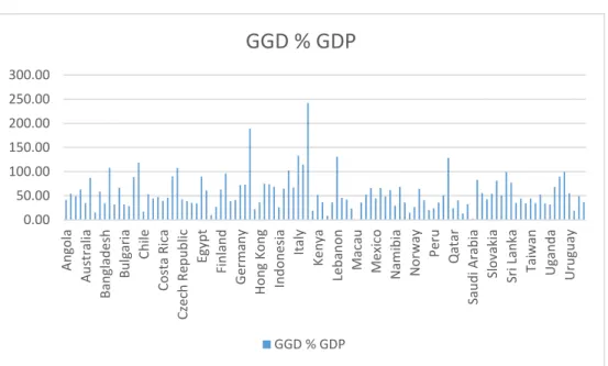
Sovereign borrowing has been an important toll among the global financial assets for hundreds of years to finance investment or respond to a cyclical crisis. As of 2010 public debt was about 19% of global financial assets (Tomz and Wright, 2012). Figure 1 shows the government gross debt (GGD) to gross domestic product (GDP) ratio of the countries used in this study. Japan has the biggest ratio with 245% and Macau has the smallest

(0%)2. Sovereign debt refers to the debt incurred by national governments

and certain fiscally autonomous territories and like other types of debt it is a contractual obligation. It covers the bank loans, treasury bills, bonds, International Monetary Fund loans, International Bank for Reconstruction and Development loans (World Bank) and loans to other official or private

2 _{IMF, International Monetary Fund, “World Economic Outlook Database", April 2016 and}

5

creditors (Beers and Nadeau, 2015)3. Like any other debt there exists

concepts such as its maturity and currency type of sovereign debt. From the initial disbursement of debt up to the date of the last principal payment is the generally accepted definition of maturity term for sovereign debt. On the other hand, an important percentage of the global sovereign debt is in foreign currency and substantially denominated in reserve currencies (U.S. dollars, Euro, Yen) of the world (Tomz and Wright, 2012). Hatchondo, Martinez and Sapriza (2007) draw attention to the insecurity of the sovereign debt. Unlike the private debtors there is no authority that can force the sovereign to pay its debt. Compared with private agents the government forces these agents to hand over the assets posted as collateral when a private agent defaults.

Figure 1: Government Gross Debt to Gross Domestic Product

Source: IMF World Economic Outlook

3 _{See Beers and Nadeau (2015) for further description about creditor subcategories}

0.00 50.00 100.00 150.00 200.00 250.00 300.00 An go la Au st ral ia Ba ng lad es h Bul ga ria Ch ile Co st a Ri ca Cz ec h R ep ub lic Eg yp t Fi nl an d Ge rma ny Ho ng K on g In do ne sia Italy Ke ny a Le ba no n M ac au M ex ico Nami bi a No rw ay Pe ru Q at ar Sau di Ar ab ia Sl ov ak ia Sr i L an ka Ta iw an Ug an da Ur ug uay

GGD % GDP

6

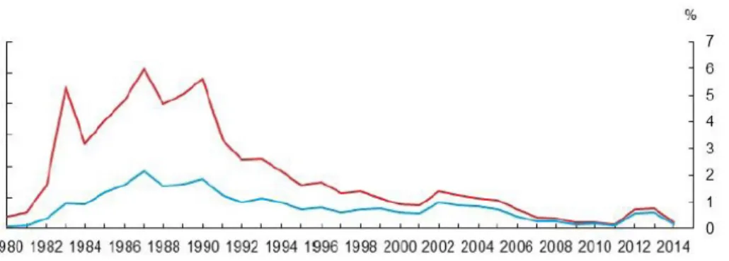
Sovereign default has an extensive history. In 1920s there was a huge explosion in sovereign debt resulting a wave of defaults during great depression (Cantor and Packer, 1995). See Figure 2 for the sovereign debt in

default as a share of world public debt and world GDP4. Sovereign default

can be defined as the violation of the legal terms of the debt contract by the debtor. Sovereign debt appears in two ways in the literature. Within the meanings of law, default occurs when the scheduled debt service is not paid beyond a grace period specified in the debt contract (Panizza, Sturzenegger and Zettelmeyer, 2009). Sovereign default is considered from a perspective of rating agencies in the studies of Peter (2002) and Bhatia (2002). In this sense it means any missed or delayed payment of interest and/or principal or any rescheduling, exchange or other restructuring of debt instrument where the debtor offers the creditor a new contract that amounts to a diminished financial obligation. Restructuring the Greek sovereign debt in 2012 is an example to second part. It can be defined as exchange of outstanding sovereign debt instruments for new debt instruments (Das, Papaioannou and Trebesch, 2012). This study uses the definition of the rating agencies. According to studies in history sovereign default does not represent high borrowing costs for countries. For the purpose of this study the reasons and

borrowing costs of sovereign defaults are not included in the paper5_.

4 _{CRAG, Bank of Canada’s Credit Rating Assesment Group, “Database of Sovereign}

Default”,March 2015

5 _{See Wright (2001), Reinhart and Rogoff (2009, 2010), Sturzennegger and Zettelmeyer}

(2007), Bulow and Rogoff (1989), Panizza, Sturzennegger and Zettelmeyer (2005) for detailed information about economies of sovereign default

7

Figure 2: Sovereign Debt in Defaults as a Share of World Public Debt and World GDP

Source: Database of Sovereign Defaults by Beers and Nadeau

Sovereign ratings are important tools for the countries to reach the international capital markets since many investors prefer rated securities instead of unrated securities at the same risk level. Therefore, governments and corporate companies want to be rated to ease their own access to capital markets. On the other hand, it is also important for the borrowers of the same nationality. Generally sovereign rating is a ceiling for the other borrowers that are resident in that country there are specific conditions to be rated above that and only few companies can be rated higher than sovereign rating. The meaning of sovereign rating is the same everywhere, like other credit ratings, and it is the assessment of likelihood of a sovereign’s ability and willingness to repay its debt and the assessment of likelihood of default. There are three major rating agencies in the world: S&P, Moody’s and Fitch Ratings. They underline that their ratings are the indicators of the creditworthiness of the rated entity rather than default risk, but still

8

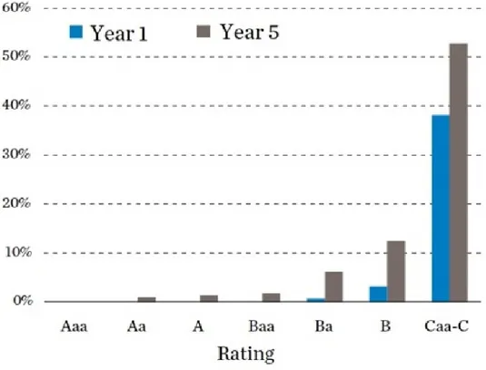
sovereign ratings and PDs are coherent in history and ratings are serious signs for PD. Figure 3 shows the sovereign default rates for each rating level6.

Figure 3: Sovereign Default Rates for Each Country Level

Source: Moody’s Sovereign Default Study 1983-2013

Sovereign credit ratings of S&P, Moody’s and Fitch indicate the capacity and willingness of rated governments to repay commercial debt obligations in full and on time. By obligor, the ratings focus exclusively on the creditworthiness of central governments, providing an assessment of

9

sovereign risk and generally serve as a ceiling for other ratings within the jurisdiction. By obligation, the ratings focus exclusively on the creditworthiness of sovereign debt to official creditors.

Sovereign ratings first started to be issued in 1900s. Today there are more than 100 countries rated by major three rating agencies (Bhatia, 2002). Rating scores are expressed in letters A, B, C, D. The top rating is “AAA” and the bottom “D” for S&P and Fitch ratings. The best is “Aaa” and the

worst “D” for the Moody’s ratings. Governments rated above “BBB-” or

“Baa3” are known as investment grade and while those rated below fall into the speculative grade category. S&P and Fitch uses (+) and (-) and Moody’s uses 1, 2 and 3 to differentiate the ratings in the same category and all three agencies have “negative” and “positive” concepts to point out the outlook of the sovereign. In addition the agencies recognize four classes for the type of indebtedness: Long-Term Foreign Currency, Short-Term Foreign Currency,

Long-Term Local Currency and Short-Term Local Currency7.The most

important is the long term foreign currency debt and the credit rating of a country refers to this class of debt unless specified otherwise. Table 1 shows the long term issuer credit rating scale of Fitch Rating. Although the presentation of the ratings is different for each agency, the definitions are the same.

7 _{Fitch Ratings, “Definitions of Ratings and Other Forms of Opinion”, December 2014,}

Moody’s Investor Service, “Ratings Symbols and Definitions”, May 2016, Standard and Poor’s, “Business and Financial Terms”, July 2014

10

Table 1: Fitch Rating Long Term Foreign Currency Rating Scale

Rating Levels of Credit Risk AAA highest credit quality AA+

very high credit quality AA

AA- A+

high credit quality A

A- BBB+

good credit quality BBB BBB- BB+ speculative BB BB- B+ highly speculative B B- CCC

high levels of credit risk CC

C

RD restricted default

D default

Source: Fitch Ratings

Rating agencies look at very large number of indicators when assessing a sovereign’s credit risk including quantitative and qualitative. They are using more than 20 economic, financial and qualitative factors. General macroeconomic indicators are the important determinants of sovereign ratings. Furthermore indicators contain measures of fiscal strength (fiscal balance, public debt, and interest cost burdens), economic strength (GDP per capita, GDP growth and inflation), political risk (governance, the rule of law, corruption and ease of doing business), the banking and monetary regime (exchange rate volatility, reserve currency status, non-performing

11

loans of gross bank loans) and other factors such as total reserves, external

debt, trade openness, unemployment and credit to GDP8_{. Rating agencies do}

not declare how they weight each indicator to reach final score; hence the subjectivity of the assessment is a point that should be considered. Although the indicators are not weighted in the same way by the all rating agencies, there is no big difference on the sovereign ratings of three agencies. For example, generally there are one or two notch differences on the ratings. This is highly due to the values of the factors make the same effect on credit rating. For example, high and volatile inflation indicates high risk for all rating agencies. After the financial crises of the decade it is seen that qualitative factors are given more importance by the rating agencies.

This paper performs an empirical analysis of long term foreign currency sovereign ratings using December 2015 rating data from Fitch Ratings. Exhaustive panel data set on macroeconomic data average and cross section data on qualitative variables and sovereign ratings for a more than 100 countries are included in the study. The main contribution of this study to the literature is to help better understand the quantitative and qualitative determinants of sovereign ratings assigned by rating agencies. It covers the larger number of countries than earlier studies also some qualitative variables are included in the study depending on developments in recent years. Regarding the empirical modeling strategy, this study uses linear

12

regression methods on a linear transformation of the ratings. Two different scenarios have been developed considering the structural differences between advanced and emerging countries. Including nine explanatory variables in existing scenario for all the countries have been seen inadequate to explain the dependent variable when it was applied for only developing countries. Therefore, two other factors were added to the model for the scenario of only emerging countries. On the other hand, a third scenario was not developed for advanced economies due to the cross section data resulting insufficient number of observations for advanced economies.

As a result, explanatory variables of both scenarios (nine variables for Scenario 1 and eleven variables for Scenario 2) are quite powerful to explain dependent variable with close to 80% R square. Also the signs of the coefficients of all independent variables in both scenarios have impact in the right direction on dependent variable which means linear transformation of sovereign ratings.

In the following sections of this study are planned to elaborate the literature about finding the determinants of sovereign ratings and the factors affecting the sovereign risk in Section 2, then data and methodology used in this paper will be detailed in Section 3 and Section 4 respectively, results of the regression analysis will be presented in Section 5 and finally the main findings of the study will be summarized in Section 6.

13

2. Review of the Literature

When looking at the literature we see that there are some similarities between measuring the credit risk of a corporate company and measuring the credit risk of a sovereign. The most important difference about working on sovereign credit risk is dependent variable. Unlike the studies of Altman (1968, 1977) and others on credit risk measurement of a company, using the defaulted countries as a dependent variable is not possible to measure sovereign risk. Because, there will not be a sufficient data for defaulted countries in the same time period of explanatory variables. Even it is possible to find a sufficient number of historical data of defaulted countries for example since 1975, this time it is unlikely to collect data about explanatory variables for all countries since that time. For that reason, studies about sovereign risk concentrated on finding the significant determinants of sovereign risk and sovereign risk ratings rather than the measurement of credit risk or prediction of a sovereign default.

There are ample studies regarding the literature on country risk and sovereign risk dating back to 1970s. Econometric approaches to identify determinants of country risk or sovereign risk are various including discriminant analysis, principal component analysis, logit analysis, G-LOGIT, probit analysis, tobit analysis, CART, ANN, hybrid neural

networks and multiple regression9_{. When narrowing the studies that only}

9 _{Nath (2008), “Country Risk Analysis: A Survey of the Quantitative Methods”, October}

14

cover sovereign ratings, the study of Cantor and Packer (1996) and models of linear regression and ordered probit are considered and accepted as the first study and as the two major econometric approaches on the determinants of sovereign ratings respectively. Following studies on the determinants of sovereign ratings are based on the study of Cantor and Packer (1996) and these two statistical methods.

In their studies Cantor and Packer (1996), they used regression analysis to measure the relative significance of eight variables that are repeatedly cited in rating agency reports of Moody’s and Standard and Poor’s until 1995 as determinants of the September 29, 1995, sovereign ratings of forty nine countries (23 industrial and 26 developing). The dependent variable used in the regression is the linear transformation of sovereign ratings and the independent variables used in the regression are GDP per capita, GDP growth, inflation, fiscal balance, external balance, external debt, economic development and default history.

They put forward that the greater GDP per capita refers to the greater tax base and it eases to repay debt. In addition, they said a relatively high rate of GDP growth suggests that a country’s burden of debt service will be easier in time. High inflation is considered as structural problems in the government’s finance and public dissatisfaction with inflation may in turn lead to political instability. It has been expressed that high budget deficits may have a negative impact on debt service by absorbing the domestic

15

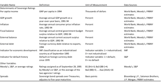
savings. Current account deficit on the other hand indicates that the economy relies on funds from abroad and it may cause an increase in foreign indebtedness and become unsustainable over time. The higher debt burden was taken as a sign for a higher risk of default. If a country’s foreign currency debt raises relative to it is foreign currency earnings, the weight of the debt burden increases. Also they used two dummy variables. First, countries may be less likely to default after a certain level of development. They looked at International Money Fund (IMF) definition if a country is classified as industrialized. Second, a country has defaulted on debt in the recent past indicates a bad reputation and defaulted sovereigns suffers a severe decline in their standing with creditors. Table 2 shows the explanatory variables and its definitions used by Cantor and Packer (1996) to measure significance of them as determinants of sovereign ratings of Moody’s and Standard and Poor’s.

Table 2: Description of Variables

Variable Name Definition Unit of Measurement Data Sources Determinants of Sovereign Ratings

Per capita income GNP per capita in 1994 Thousands of dollars World Bank, Moody's, FRBNY estimates

GDP growth Average annual GDP growth on a Percent World Bank, Moody's, FRBNY year-over-year basis, 1991-94 estimates

Inflation Average annual consumer price inflation Percent World Bank, Moody's, FRBNY rate, 1992-94 estimates

Fiscal balance Average annual central government budget Percent World Bank, Moody's, FRBNY surplus relative to GDP, 1992-94 estimates

External balance Average annual current account surplus Percent World Bank, Moody's, FRBNY relative to GDP, 1992-94 estimates

External debt Foreign currency debt relative to exports, Percent World Bank, Moody's, FRBNY

1994 estimates

Indicator for economic development IMF classification as an industrialized Indicator variable: 1 = industrialized; IMF country as of September 1995 0 = not industrialized

Indicator for default history Default on foreign currency debt Indicator variable: 1 = default; S&P since 1970 0 = no default

Other Variables

Moody's, S&P, or average ratings Ratings assigned as of September 29, 1995 B1 (B+)=3; Ba3 (BB-)=4; Moody's, S&P by Moody's or S&P, or the average of the Ba2 (BB)=5; ... Aaa (AAA)=16

two agencies' ratings

Spreads Sovereign bond spreads over Treasuries, Basis points Bloomberg L.P., Salomon Brothers, adjustes to five-year maturities J.P. Morgan, FRBNY estimates

16

Their study showed that five of the eight variables are directly correlated with the ratings assigned by Moody’s and Standard and Poor’s. GDP per capita, inflation, external debt, economic development and default history are consistently related to higher ratings. The other three variables consisting of GDP growth, fiscal balance and external balance were deemed inadequate to explain sovereign ratings. The lack of correlation between GDP growth and sovereign ratings was stated understandable due to the rapid growth of developing countries. Adjusted R square of the estimation is 92.4% indicating that regression of the average of Moody’s and Standard and Poor’s ratings against their set of eight variables explains more than 90 percent of the sample variation and yields a residual standard error of about 1.2 rating notches.

Considering the year of the study, the number of the countries rated and the globalization effect on the international capital markets after this study, it can be said that determinants of the sovereign ratings and the weights of determinants may change in time.

Monfort and Mulder (2000) focused on the study of currency crises and a few external indicators like foreign reserves, current account balance (CAB) and exports played an important role in their paper. They estimated and presented a model of ratings for sovereigns of emerging market economies focusing on sovereign ratings for 20 of the larger emerging market economies on a semiannual basis from 1994-99 to examine the nature of the

17

ratings and the degree of procyclicality. They also used regression analysis and the ratings of Moody’s and Standard and Poor’s as Cantor and Packer (1996).

Hu, Kiesel and Perraudin (2000) showed how one may estimate transition probabilities for an important class of sovereign issuers. To put it more explicitly their approach consists of modeling sovereign defaults and Standard and Poor’s sovereign ratings within a common maximum likelihood, ordered probit framework. They included ten variables in the most general models that they estimated. Default history, lower reserves, higher inflation, higher debt to gross national product, being a developing country and higher ratio of debt service to exports contribute to lower credit quality.

Afonso (2003) estimated the equation using ordinary least squares (OLS) as Cantor and Packer to find the factors to play an important role in determining sovereign debt rating. He used the linear and logistic transformation of rating classifications of S&P and Moody’s (June 2001) for a sample consisting 81 countries (29 developed and 52 developing).

Bissoondoyal-Bheenick (2005) used ordered response models for 95 countries which is divided into two broad samples where the first sample consisted of high rated 25 countries and the second sample consisted of low

18

rated 70 countries. Also he used some other macroeconomic performance variables such as unemployment rate and investment to GDP ratio.

Butler and Fauver (2006) used credit rating data from Institutional Investor for a sample of 86 countries to examine the cross sectional determinants of sovereign credit ratings. They explained the Institutional Investor credit ratings as a numerical rating that ranges from zero to hundred. In their paper they found that the quality of a country’s legal and political institutions plays a vital role in determining the sovereign credit ratings.

Depken, LaFountain and Butters (2006) measured the impact of corruption on a country’s creditworthiness or willingness and ability to repay its sovereign debts. Their study showed us variables that assess political risk like corruption, political stability or rule of law can also be relevant to the sovereign risk or sovereign ratings as well as the indicators of fiscal policy, budget balance and government debt. They used S&P’s issuer credit ratings as a dependent variable and similar independent variables used in other analysis of sovereign credit ratings in literature. They found that public corruption reduces creditworthiness of a country as measured by sovereign credit ratings.

Afonso, Gomes and Rother (2011) performed an empirical analysis of foreign currency debt ratings using rating data from Fitch Ratings, Moody’s and Standard and Poor’s. They collected panel data set for sovereign ratings,

19

macroeconomic data and qualitative variables starting from1995. They used both linear regression and ordered probit methods to estimate determinants. The results of the models showed that GDP per capita, GDP growth, public debt and government balance have short run impact; government effectiveness, external debt and external reserves have long run impact on sovereign ratings.

When comparing the models relative to each other, it is clear that regression methods are pretty simple and enable a straightforward generalization to panel data through fixed or random effects estimation. Even though estimating the determinants of ratings using linear regression approaches has in general a good fit and a good predictive power it faces some critiques. As ratings are qualitative ordinal measures, using traditional estimation techniques on a linear transformation of the ratings is not the most adequate framework of estimation. The inadequacy is derived from the assumption that the difference between two rating categories is equal for any two contiguous categories and that the existence of elements at the top and

bottom categories makes the assumption biased. Ordered response models

were being used in response to this. However, it cannot be generalized for a small sample. So if the determinants of the ratings will be estimated using a cross section of countries where there are too few observations, it is very important to try to maximize the number of observation by using panel data. But the generalization of ordered probit to panel data is not simple due to the existence of country specific effect. Furthermore, the need to have many

20

observations makes it harder to perform robustness analysis (Afonso et al., 2011).

After the internal model to calculate regulatory capital for banks becomes important it is expected that there will be an increase in the studies on this

subject10. Internal approach means using an internal scoring model rather

than rating agencies. In addition, hybrid models will be preferred instead of point-in-time models. Also forecasting values of the determinants will be used to explain sovereign ratings.

10 _{Basel Committee on Banking Supervision, “Revisions to the Standardized Approach for}

21

3. Data

In this study data collection started with sovereign credit ratings and Fitch Ratings’ long term foreign currency ratings on issuer in December 2015 were used for statistical analysis. As mentioned in introduction this class of credit rating shows Fitch Ratings’ opinion of single borrower’s creditworthiness on long term debt (having a term of more than one year) which is denominated in foreign currency. The underlying reason of preferring this class is that ratings are forward looking opinions including views of future performance and most of the public debt of countries is denominated in foreign currency. Just like the other rating agencies Fitch Ratings may also update or withdraw a country’s rating and assign a rating for a country that is not rated before. Also it may change country’s outlook or rating watch. Unless there is an exceptional case or a strong change in macroeconomics of a country they do not update ratings in a time period shorter than six months.

As of December 2015 sovereign ratings assigned by Fitch Ratings were available for 111 countries or autonomous region. Appendix 1 reports the ratings assigned by Fitch Ratings to 111 sovereigns in December 2015. Abu Dhabi, Andorra and San Marino are eliminated because of the lack of some explanatory variables. Private credit as a percentage of GDP, Current Account Balance to GDP and government indicators are absent for these countries respectively. Elimination of Abu Dhabi, Andorra and San Marino reduced the sample size to 108. According to scenarios generated in this

22

paper there are two samples including all countries sample size of 108 and emerging countries sample size of 72. The list of countries that are classified as advanced and emerging countries in this study are shown in Table 3 and Table 4 respectively. Classification of the countries are described in the explanatory variables section below.

Table 3: Advanced Economies

Australia France Korea Singapore

Austria Germany Latvia Slovakia

Belgium Greece Lithuania Slovenia

Canada Hong Kong Luxembourg Spain

Cyprus Iceland Malta Sweden

Czech Republic Ireland Netherlands Switzerland

Denmark Israel New Zealand Taiwan

Estonia Italy Norway United Kingdom

Finland Japan Portugal United States

Source: IMF

Table 4: Emerging Countries

Angola Croatia Lebanon Romania

Argentina Dominican Republic Lesotho Russia

Armenia Ecuador Macau Rwanda

Aruba Egypt Macedonia Saudi Arabia

Azerbaijan El Salvador Malaysia Serbia

Bahrain Ethiopia Mexico Seychelles

Bangladesh Gabon Mongolia South Africa

Bolivia Georgia Morocco Sri Lanka

Brazil Ghana Mozambique Suriname

Bulgaria Guatemala Namibia Thailand

Cameroon Hungary Nigeria Tunisia

Cape Verde India Pakistan Turkey

Chile Indonesia Panama Uganda

China Iraq Paraguay Ukraine

Colombia Jamaica Peru Uruguay

Congo, Republic of Kazakhstan Philippines Venezuela

Costa Rica Kenya Poland Vietnam

Cote d'Ivoire Kuwait Qatar Zambia

23

It is accepted that macroeconomic and financial dynamics and governance indicators are important determinants of sovereign credit ratings similarly to the proposal of the literature. Nevertheless, volatility of GDP is substituted for GDP growth since it is higher for the emerging countries than the advanced economies because they tend to grow faster. Besides the correlation between GDP growth and the sovereign ratings is found opposite contrary to expectations. The explanatory variables applied in this study for the whole population of 108 countries to assess determinants of sovereign ratings are governance (consisting of percentile expression of political stability and rule of law), GDP per capita, volatility of GDP, inflation, general government balance (GGB) to GDP, current account balance (CAB) to GDP, government gross debt (GGD) to GDP. Moreover, the sample of the 72 developing countries include net sovereign foreign currency (FX) position as a percentage of GDP and private credit to GDP.

Lastly development level and default history were included for use as dummy variables whether a country is developed or not and whether it has defaulted before or not. Macroeconomic and financial data of countries were collected mostly from World Bank (WB) and International Monetary Fund. Governance indicators were obtained from worldwide governance indicators data of World Bank. Advanced economies definition of IMF was used to separate countries as developed or emerging. Finally default history data was provided from CRAG database for sovereign default. Missing data was supplemented from data in the Fitch Ratings December 2015 Sovereign

24

Data Comparator. According to IMF and WB, definitions and theoretical explanations about the set of explanatory variables that affects sovereign ratings will be presented in the following.

Governance indicator was calculated by taking the average of the percentile expressions of political stability and rule of law. Political stability evaluates the performance of political power and the tendency of violence and terrorism in a country. Rule of law expresses the applicability of the legal system in fair and equitable manner against the whole society. Also it covers the quality of contracts, property rights, police unit, courts and crime rate. Governance indicator refers to the political risk.

GDP per capita is a measure of GDP (in current dollars) divided by the total population. Obviously countries with higher per capita income are more likely to repay its debt.

Volatility of GDP is standard deviation of the GDP growth over the last ten years. GDP growth is higher in the developing countries since they are eager to grow faster. Their volatility of GDP growth is greater than the developed countries at the same time. High volatility of GDP indicates economic instability.

Inflation (CPI) refers to the average annual change in consumer prices. It is calculated based on real values of previous years in percentage terms.

25

Higher inflation means that the government’s finances are not in good order and it can lead to political instability (Cantor and Packer, 1996).

General Government Balance (GGB) to GDP is also known as fiscal balance to GDP. GGB is calculated by taking difference between government expenditures and government revenues. This balance can be seen as a factor showing the effect of general government activities on remaining players of economy.

Current Account Balance (CAB) to GDP is also known as external balance to GDP. The current account is all transactions excluding financial and capital items. Basic classification is exports and imports with income receipts and income payments. Focus on the balance of payments is all transfers in goods and services and income.

Both GGB to GDP and CAB to GDP have to be positive for sign of good economy. Countries with fiscal deficits and current account deficits are perceived that they may not repay their debt service.

Government Gross Debt (GGD) to GDP consists of all principle and interest payments which will be paid at the maturity or in the future. It includes special drawing rights, foreign currency deposits, debt securities, pension and standard guarantee programs and other undocumented debts. Clear from the name high gross debt means high risk.

26

Net Sovereign FX Position to GDP is net sovereign FX debt expressed as a percentage of GDP. Net sovereign FX debt is general government plus central bank FX denominated debt, less FX denominated assets. If it is negative it means sovereign FX assets are bigger than FX debt liabilities. Countries with higher sovereign assets are more likely to repay their FX debt liabilities.

Private Credit to GDP is domestic credit to private sector as a percentage of GDP. Domestic credit to private sector indicates the financial resources provided to the private sector by financial corporations such as loans, purchases of non-equity securities, trade credits and other accounts receivable that establish a claim for repayment. Private Credit to GDP reflects the banking system of a country.

Development level is a dummy variable. Although GDP per capita suggests an idea about the development level of a country, rating agencies assign a smaller PD to the developed countries. IMF country classification is presented in Appendix 2. Indicator variable is equal to 1 if a country is classified under advanced economies and is equal to 0 otherwise. Note that it was not used for second scenario since it covers only the countries outside of the advanced economies.

Default History is another dummy variable indicating that countries have defaulted on debt in the recent past are perceived as having a bad reputation

27

and a high credit risk (Cantor and Packer, 1996). Indicator variable is equal 1 if a country has defaulted at least once since 1975 and is equal to 0

otherwise. Table 5 presents the defaulted countries in this study11.

Table 5: Defaulted Countries since 1975

Argentina Egypt Nigeria Seychelles

Bolivia Gabon Panama South Africa

Brazil Greece Paraguay Turkey

Cameroon Kenya Peru Uganda

Chile Mexico Poland Ukraine

Congo, Republic of Mongolia Romania Uruguay

Costa Rica Morocco Russia Venezuela

Cote d'Ivoire Mozambique Serbia Zambia

Dominican Republic

Ecuador

Source: CRAG Database

The average values between 2010 and 2015 were used for CPI, GGB to GDP, CAB to GDP, GGD to GDP, net sovereign FX position to GDP and private credit to GDP to avoid outliers and make an assessment about recent years.

Explanatory variables used in this paper are shown in Table 6.

28

Table 6: Explanatory Variables

Variable Name Unit of Measurement Data Sources

Governance Percentile WB, World Governance Indicators

GDP per capita USD dollar IMF World Economic Outlook

Vol of GDP Growth Percent IMF World Economic Outlook

CPI Percent IMF World Economic Outlook

GGB Percent IMF World Economic Outlook

CAB Percent IMF World Economic Outlook

GGD Percent IMF World Economic Outlook

Net Sov FX Pos to

GDP Percent Fitch Ratigs Sovereign Data Comparator Private Credit to

GDP Percent WB, World Government Indicators

Development

Level 1=advanced 0=otherwise IMF

Default History 1=default 0=otherwise CRAG

29

4. Methodology

Multiple Linear Regression Model is approved to analyze the detected determinants of sovereign ratings. Multiple Linear Regression is a statistical tool to describe and evaluate the relationship between a given independent variable and more than one other explanatory variable by using the OLS estimators for parameters and their standard errors (Brooks, 2008).

To illustrate the model, generalized formula of the multiple regression equation is given below.

𝑦𝑦𝑡𝑡 = 𝛽𝛽1+ 𝛽𝛽2𝑥𝑥2𝑡𝑡 + 𝛽𝛽3𝑥𝑥3𝑡𝑡+ ⋯ + 𝛽𝛽𝑘𝑘𝑥𝑥𝑘𝑘𝑡𝑡+ 𝑢𝑢𝑡𝑡, 𝑡𝑡 = 1, 2, … , 𝑇𝑇

The variables 𝑥𝑥_2𝑡𝑡, 𝑥𝑥_3𝑡𝑡, … , 𝑥𝑥_{𝑘𝑘𝑡𝑡} are a set of 𝑘𝑘 − 1 explanatory variables which

are thought to influence 𝑦𝑦, and the coefficient estimates 𝛽𝛽₁, 𝛽𝛽₂, … , 𝛽𝛽_𝑘𝑘 are the

parameters which quantify the effect of each of these explanatory variables

on 𝑦𝑦. Note that,𝑥𝑥₁ is not included in the formula since it stands for the

constant term and usually represented by a column of ones of length 𝑇𝑇

(Brooks, 2008).

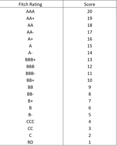
The method of linear transformation of issuer rating scales is used to

identify dependent variable (𝑦𝑦) of the model (Cantor and Packer, 1996;

Bhatia, 2002). Table 7 shows the linear transformation of Fitch Ratings Scale.

30

Table 7: Linear Transformation of Issuer Rating Scales

Fitch Rating Score

AAA 20 AA+ 19 AA 18 AA- 17 A+ 16 A 15 A- 14 BBB+ 13 BBB 12 BBB- 11 BB+ 10 BB 9 BB- 8 B+ 7 B 6 B- 5 CCC 4 CC 3 C 2 RD 1

OLS is the estimation technique that is used in regression models and it has to have some desirable properties. For this purpose, there are several assumptions relating to multiple linear regression model. Moreover, there are other implicit assumptions to show the coefficient estimates could validly be conducted. These are multicollinearity, adopting the wrong functional form, omission of an important variable and inclusion of an irrelevant variable. The assumptions of multiple linear regression are as

follows12.

12 _{See Chapter 3 and Chapter 4 of Brooks (2008) for detailed explanation about multiple}

31

1. Average value of the errors is zero

2. Homoscedasticity: The variance of the errors is constant 3. Covariance between the error terms over time is zero

4. 𝑥𝑥_𝑡𝑡 are nonstochastic

5. Normality: The disturbances are normally distributed

In the case of this thesis, there are dummy variables. The difference between a dummy variable and other explanatory variables is that they are numerical expressions of a qualitative entity and in most condition only zero and one are used to represent the qualitative entity and the opposite of it.

32

5. Results

The main goal in this study is creating a multiple regression model by using statistical technique of OLS to understand the determinants of sovereign risk of a country which is evaluated by rating agencies. For this purpose, 9 macroeconomic indicators and 2 qualitative factors considered to explain the sovereign ratings or/and reflect the sovereign risk of a country are determined and two scenarios were developed because of the structural differences of countries.

In the first scenario, ratings of 108 countries were used as the dependent variables and 7 indicators and 2 qualitative factors were used as explanatory variables. In the determination, correlation between ratios and sovereign rating scores which is transformation of ratings and previous literature was effective. Explanatory variables according to correlation with rating scores and the literature were governance, GDP per capita, volatility of GDP, inflation, GGB to GDP, CAB to GDP, GGD to GDP, development level and default history. Unlike the literature, volatility of GDP was used instead of GDP growth. As stated in literature, GDP growth is not significant to explain sovereign ratings. Because the emerging countries which have lower ratings than advanced economies tend to grow faster.

All ratios used in the study for the first scenario were in the right direction with rating scores contrary the study of Cantor and Packer (1996). However, volatility of GDP and GGD to GDP has really small correlation.

33

When applying the model which is used in Scenario 1 to only emerging countries (all countries except advanced economics), it was seen that the indicators were inadequate to explain rating scores with nearly 60% R square. Therefore, two another ratios (net sovereign FX position to GDP and private credit to GDP) were added and Scenario 2 was generated.

In the second scenario, all ratios except volatility of GDP have significant correlation with rating scores. So, multiple regression model was applied for two scenarios and these scenarios are as follows:

Scenario 1: Model for 108 countries by using 9 explanatory variables with 2 as dummy (development level and default history)

Scenario 2: Model for 72 emerging countries by using 10 explanatory variables with 1 as dummy (default history)

The Eviews software was used to make estimations for the multiple regression equations and apply diagnostic tests to interpret the statistical adequacy of models. According the Eviews outputs the results are below.

34

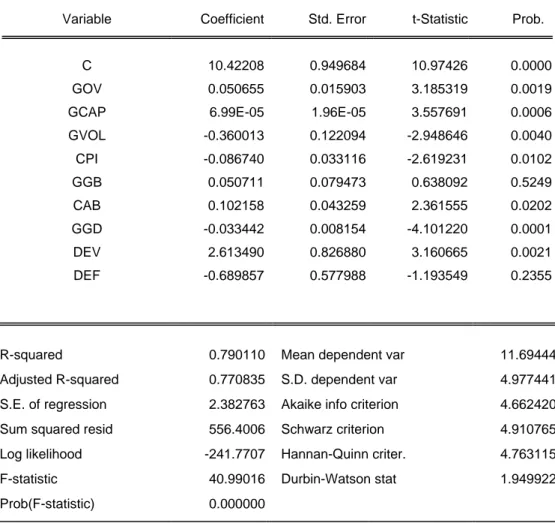
Scenario 1: Model estimated for 108 countries by using 9 explanatory variables with 2 as dummies (development level and default history). Table 8 shows the estimation output of Scenario 1.

Scenario 1 is considered as base scenario in the literature. Almost all studies on the determinants of sovereign risk used these macroeconomic indicators starting from Cantor and Packer (1996) to Afonso at al. (2011) with some changes. Unlike the literature, volatility of GDP was added to the model. Because GDP growth was insignificant since it is lower in highly rated countries. Volatility of GDP may be a good indicator since it reflects the economic stability.

Dependent Variable:

SCORE = Linear transformation of Fitch sovereign ratings in Dec. 2015 Explanatory Variables:

GOV = Governance GCAP = GDP per capita

GVOL = Volatility of GDP growth CPI = Inflation

GGB = GGB to GDP ratio CAB = CAB to GDP ratio GGD = GGD to GDP ratio DEV = Development level DEF = Default history

35

Table 8: Estimation Output (Scenario 1)

Dependent Variable: SCORE Method: Least Squares Date: 05/24/16 Time: 23:42 Sample: 1 108

Included observations: 108

Variable Coefficient Std. Error t-Statistic Prob. C 10.42208 0.949684 10.97426 0.0000 GOV 0.050655 0.015903 3.185319 0.0019 GCAP 6.99E-05 1.96E-05 3.557691 0.0006 GVOL -0.360013 0.122094 -2.948646 0.0040 CPI -0.086740 0.033116 -2.619231 0.0102 GGB 0.050711 0.079473 0.638092 0.5249 CAB 0.102158 0.043259 2.361555 0.0202 GGD -0.033442 0.008154 -4.101220 0.0001 DEV 2.613490 0.826880 3.160665 0.0021 DEF -0.689857 0.577988 -1.193549 0.2355

According to estimation output of Eviews all the coefficients have their expected signs (See Section 3). Moreover, the coefficients of governance, GDP per capita, volatility of GDP, GGD to GDP and development level are significant at 1% confidence level. The coefficients of inflation and CAB to GDP are significant at 5% confidence level. However, GGB to GDP and

R-squared 0.790110 Mean dependent var 11.69444 Adjusted R-squared 0.770835 S.D. dependent var 4.977441 S.E. of regression 2.382763 Akaike info criterion 4.662420 Sum squared resid 556.4006 Schwarz criterion 4.910765 Log likelihood -241.7707 Hannan-Quinn criter. 4.763115 F-statistic 40.99016 Durbin-Watson stat 1.949922 Prob(F-statistic) 0.000000

36

default history are statistically insignificant. Cantor and Packer (1996) explain that in some cases the market forces countries to have strong fiscal and external balances diminishing the significance of the coefficients of fiscal and external balances.

Testing Multiple Hypothesis and Goodness of Fit

T statistics of the coefficients in Table 8 shows the significance level of only one coefficient. F statistics on the other hand is a joint test to understand if the coefficients are jointly significant or not. If F statistic is smaller than the confidence level the joint null hypothesis (all of the slope parameters are jointly zero) should be rejected.

Goodness of fit statistics says how well the independent variables explain

the dependent variable. 𝑅𝑅2 is one of the tools to measure goodness of fit. It

is a value lying between 0 and 1. If it is close to 1 the model fits the data well. Second part of Table 8 shows the F statistic and goodness of fit results of estimation in Scenario 1.

Since probability of F statistic is smaller than 0.05 the null hypothesis is

rejected. So the coefficients in Scenario 1 are jointly significant. Also 𝑅𝑅2 is

79% pointing that multiple regression model created for the pool of all countries fits the data well.

37

Assumption of Homoscedasticity

Assumption of homoscedasticity says that the variance of the errors is constant otherwise they are said to be heteroscedastic. There are several methods to run a statistical test for heteroscedasticity. White’s test is one of them (White, 1980). There are three version of the statistic: F-statistic, Obs*R-squared and Scaled explained SS. Three of them say the same if test statistic exceeds the critical value, the null hypothesis (there is heteroscedasticity) should be rejected. Table 9 shows the White test results for Scenario 1.

Table 9: Heteroscedasticity Test (Scenario 1)

Heteroskedasticity Test: White

F-statistic 1.449506 Prob. F(9,98) 0.1778 Obs*R-squared 12.68777 Prob. Chi-Square(9) 0.1773 Scaled explained SS 11.03908 Prob. Chi-Square(9) 0.2730

Since probability of test statistics of three versions are bigger than 0.05, null hypothesis is rejected. So there is no heteroscedasticity.

Assumption of Normality

Assumption of Normality requires that the disturbances are normally distributed. Jarque-Bera is the most common test applied for normality (Jarque and Bera, 1987). It is a measure of the transformation of kurtosis

38

and skewness. If the test statistic is bigger than the 0.05 critical value, the null hypothesis (normality) should not be rejected. Figure 4 shows the Jarque-Bera Test results.

Figure 4: Jarque-Bera Test (Scenario 1)

The probability of Jarque-Bera test statistic is 0.838. Therefore, the null hypothesis is not rejected and disturbances are normally distributed.

Multicollinearity

Multicollinearity means the explanatory variables are correlated with one another. An implicit assumption for OLS estimation method is non-multicollinearity. There should not be a significant relationship between the explanatory variables. Table 10 shows the correlation matrix of explanatory variables used for OLS estimation in Scenario 1. According to this correlation matrix only the correlation between governance and GDP per capita may be considered as significant with 72.15%. To put it another way,

0 2 4 6 8 10 12 14 -6 -4 -2 0 2 4 6 Series: Residuals Sample 1 108 Observations 108 Mean 1.12e-15 Median -0.122897 Maximum 5.676674 Minimum -6.668525 Std. Dev. 2.280352 Skewness -0.128146 Kurtosis 3.113358 Jarque-Bera 0.353410 Probability 0.838027

39

a country with high governance indicators is expected to have high GDP per capita or vice versa.

Table 10: Correlation Matrix of Explanatory Variables (Scenario 1)

GOV GCAP GVOL CPI GGB CAB GGD GOV 1.00 0.72 0.04 -0.38 0.26 0.35 0.23 GCAP 0.72 1.00 0.15 -0.12 0.43 0.55 0.09 GVOL 0.04 0.15 1.00 0.15 0.33 0.35 -0.16 CPI -0.38 -0.12 0.15 1.00 -0.10 -0.07 -0.17 GGB 0.26 0.43 0.33 -0.10 1.00 0.62 -0.38 CAB 0.35 0.55 0.35 -0.07 0.62 1.00 -0.19 GGD 0.23 0.09 -0.16 -0.17 -0.38 -0.19 1.00

Scenario 2: Model estimated for 72 countries for by using 10 explanatory variables with 1 as dummy (default history). Table 11 shows the estimation output of Scenario 2.

Explanatory variables in Scenario 1 were inadequate to explain the sample of emerging countries with 62.7% R-square lower than the Scenario 1. Therefore, net sovereign FX position to GDP and private credit to GDP ratios was added to estimation model in Scenario 2. Both have more than 50% correlation with the scores of emerging countries.

40

Dependent Variable:

SCORE = Linear transformation of Fitch Sovereign Ratings in Dec. 2015

Explanatory Variables: GOV = Governance GCAP = GDP per capita

GVOL = Volatility of GDP growth CPI = Inflation

GGB = GGB to GDP ratio CAB = CAB to GDP ratio GGD =GGD to GDP ratio

FX = Net sovereign FX position to GDP PC = Private credit to GDP

41

Table 11: Estimation Output (Scenario 2)

Dependent Variable: SCORE Method: Least Squares Date: 05/25/16 Time: 05:26 Sample: 1 72

Included observations: 72

Variable Coefficient Std. Error t-Statistic Prob. C 8.494577 0.813368 10.44370 0.0000 GOV 0.043153 0.013154 3.280636 0.0017 GCAP 4.77E-05 2.60E-05 1.836219 0.0712 GVOL -0.247046 0.106458 -2.320602 0.0237 CPI -0.068661 0.024799 -2.768704 0.0074 GGB 0.123784 0.070036 1.767421 0.0822 CAB 0.031549 0.036144 0.872865 0.3862 GGD -0.026200 0.010981 -2.385897 0.0202 FX -0.051947 0.011256 -4.614960 0.0000 PC 0.029959 0.008031 3.730641 0.0004 DEF -0.075227 0.425570 -0.176769 0.8603

According to estimation output of Eviews all the coefficients have their expected signs (See Section 3). Furthermore, the coefficients of governance, inflation, net sovereign FX position to GDP and private credit to GDP are significant at 1% confidence level. The coefficients of volatility of GDP

R-squared 0.816183 Mean dependent var 9.319444 Adjusted R-squared 0.786049 S.D. dependent var 3.551736 S.E. of regression 1.642849 Akaike info criterion 3.970504 Sum squared resid 164.6360 Schwarz criterion 4.318328 Log likelihood -131.9381 Hannan-Quinn criter. 4.108974 F-statistic 27.08521 Durbin-Watson stat 1.787018 Prob(F-statistic) 0.000000

42

growth and GGD to GDP are significant at 5% confidence level. The coefficients of GDP per capita and GGB to GDP are significant at 10% confidence level. But the coefficients of CAB to GDP and default history are statistically insignificant. As the GGB to GDP, CAB to GDP of a country may be strong in some cases although its rating is low. This relationship is weaker for emerging market countries than the developed ones.

Testing Multiple Hypothesis and Goodness of Fit

Second part of Table 11 shows the F statistic and goodness of fit results of estimation in Scenario 2. Since the probability of F statistic is smaller than 0.05 the null hypothesis is rejected. Therefore, the coefficients in Scenario 2

are jointly significant as Scenario 1. In addition, 𝑅𝑅2 is 81.6% indicating that

multiple regression model created for emerging countries explain 81.6% of the sample.

Assumption of Homoscedasticity

White Test was used to check heteroscedasticity and the result being presented in Table 12.

43

Table 12: Heteroscedasticity Test (Scenario 2) Heteroskedasticity Test: White

F-statistic 0.649934 Prob. F(10,61) 0.7652 Obs*R-squared 6.932698 Prob. Chi-Square(10) 0.7318 Scaled explained SS 8.089804 Prob. Chi-Square(10) 0.6201

Since the probabilities of test statistics of F-Test, Obs*R-Squared and Scaled explained SS bigger than 0.05 the null hypothesis is rejected. So the disturbances are homoscedastic.

Assumption of Normality

Figure 5 shows the Jarque-Bera test result for normality. Probability is slightly up than 0.05to not reject the null hypothesis. The disturbances are normally distributed.

Figure 5: Jarque-Bera Test (Scenario 2)

0 2 4 6 8 10 12 -5 -4 -3 -2 -1 0 1 2 3 4 Series: Residuals Sample 1 72 Observations 72 Mean -3.03e-15 Median 0.049238 Maximum 3.998145 Minimum -5.374071 Std. Dev. 1.522766 Skewness -0.318311 Kurtosis 4.251405 Jarque-Bera 5.913904 Probability 0.051977

44

Multicollinearity

The most powerful relation is 62% between the GDP per capita and CAB to GDP ratio still it is not significant. Other correlations are around 50% or less.

Table 13: Correlation Matrix of Explanatory Variables (Scenario 2)

GOV GCAP GVOL CPI GGB CAB GGD FX PC

GOV 1.00 0.47 0.15 -0.31 0.23 0.19 0.02 -0.04 0.28 GCAP 0.47 1.00 0.56 0.12 0.57 0.62 -0.23 -0.32 0.24 GVOL 0.15 0.56 1.00 0.16 0.43 0.45 -0.19 -0.13 0.09 CPI -0.30 0.12 0.16 1.00 -0.10 0.02 -0.10 0.09 -0.14 GGB 0.23 0.57 0.43 -0.10 1.00 0.61 -0.49 -0.33 0.11 CAB 0.19 0.62 0.45 0.02 0.61 1.00 -0.46 -0.44 0.24 GGD 0.02 -0.23 -0.19 -0.10 -0.49 -0.46 1.00 0.44 0.04 FX -0.04 -0.32 -0.13 0.09 -0.33 -0.44 0.44 1.00 -0.42 PC 0.28 0.24 0.09 -0.14 0.11 0.24 0.04 -0.42 1.00

To sum up, multiple regression model which performed to understand significant determinants of sovereign ratings demonstrated that there is need to make a country classification when assessing the sovereign risk of countries. According to the literature and current rating studies this classification should be made for development levels of countries. Also it is seen that the existing model was not enough to explain rating scores of emerging countries. For this purpose, two scenarios were generated and results showed that when net sovereign FX position to GDP and private

credit to GDP ratios were added to the model, 𝑅𝑅2 increased from 60% to

45

As a conclusion the signs of the coefficients were correct in both two scenarios. However, GGB to GDP ratio and CAB to GDP ratio were not statistically significant in the Scenario 1 and Scenario 2 respectively. It can be explained that countries want to generate fiscal and external surplus because of the reluctance to lose their credibility. In addition, default history dummy was surprisingly insignificant for both scenarios. It may be a sign that there is no strong relationship anymore between sovereign ratings and the default history as in 1990s.

Finally, it was not easy to evaluate the statistical adequacy of the study of Cantor and Packer (1996) because of the lack of diagnostic tests. In this study some diagnostic tests were made and according to test results the disturbances are normally distributed and there is no heteroscedasticity in disturbances. Also it is possible to say there is no multicollinearity between explanatory variables. Therefore, it can be said that both models Scenario 1 and Scenario 2 are statistically adequate.

46

6. Conclusion

Sovereign risk is on the rating agencies’ agenda since 1900s. Although it slowed down during the great depression and World War 2, the number of the rated countries started to grow rapidly after the globalization movements. And nowadays, sovereign ratings became the most important tools to assess the sovereign risk. The factors are expected to affect the sovereign risk are declared by rating agencies. Nonetheless they do not declare the mathematical or statistical methods which they use or the weights of the factors which they take into account.

The studies on finding or understanding the determinants of sovereign ratings were started in 1996 with the study of Cantor and Packer and two important statistical approach were adopted to develop models in these studies. Regression methods and ordered probit methods are the methods which used in these studies.

This study uses the regression methods to find out the significance levels of the macroeconomic, financial or qualitative factors on the scores which are transformed from the sovereign ratings of Fitch Ratings in December 2015. In this study and in most of the studies in the literature dependent variable was determined in this way because of disputes regarding access to data. Also regression methods were approved since the data used in the study is cross-sectional.

47

After determining methodology, countries were classified in two groups. First group was the entire group including 108 countries and second group was the smaller group including 72 emerging countries. According to country classification two scenarios were created in order to obtain better results. 7 macroeconomic factors and 2 qualitative factors were chosen for the base scenario which covers the rating scores of 108 countries. Second scenario which consists of the rating scores of 72 emerging countries was created with the addition of net sovereign FX position and private credit to GDP and as a result it covers the 9 macroeconomic factors and 1 qualitative factor.

Quantitative and qualitative factors used in the study were chosen according to preliminary study and related literature. Therefore, highly correlated factors with sovereign ratings and the factors associated with sovereign debt and sovereign risk were used in this study. As a result of this preliminary study it is realized that GDP growth was an insignificant indicator for sovereign ratings, although almost all studies in the literature used this indicator. So volatility of GDP replaced with GDP growth considering it is a better indicator pointing the economic instability.

The factors covered by the Scenario 1 are governance, GDP per capita, volatility of GDP, inflation, GGB to GDP, CAB to GDP, GGD to GDP, development level and default history. Regression result showed that these factors are successful to explain 79% of the sample dependent variable.

48

Furthermore, all factors except fiscal balance to GDP and default history were found statistically significant. On the other hand, all the factors were jointly significant.

The factors covered by the Scenario 2 are governance, GDP per capita, volatility of GDP, inflation, GGB to GDP, CAB to GDP, GGD to GDP, net sovereign FX position to GDP, private credit to GDP and default history. As a result of regression result the factors as explanatory variables explains the 81.6% of sample dependent variable. All the coefficients of the factors except CAB to GDP and default history were found significant in Scenario 2. Similarly, the factors were jointly significant.

The success of the models is not limited with the significance levels of the explanatory variables. Moreover, the signs of the coefficients were correct. For example, increase of GDP per capita will cause an increase in rating score in both scenarios. In the same way, an increase in inflation will cause a decrease in rating scores in both scenarios.

Also some diagnostic tests were applied to multiple regression models in Scenario 1 and Scenario 2. According to these diagnostic tests models which are created to explain the sovereign ratings by using quantitative macroeconomic factors and other qualitative factors were found statistically adequate.

49

Currently sovereigns risk and sovereign ratings are hot issues after many countries trying to open their economy to the rest of the world. Also new regulations in the banking sector in the world are encouraging the development of new rating systems. For that reasons the methods to determine the macroeconomic and qualitative factors will become more important. New studies can be seen about this subject in the coming days.

50

Appendix

Appendix 1: Sovereign Ratings of Fitch Ratings in December 2015 Issuer Long Term Foreign Currency Rating

Abu Dhabi AA Andorra BBB Angola B+ Argentina RD Armenia B+ Aruba BBB- Australia AAA Austria AA+ Azerbaijan BBB- Bahrain BBB- Bangladesh BB- Belgium AA Bolivia BB Brazil BBB- Bulgaria BBB- Cameroon B Canada AAA Cape Verde B Chile A+ China A+ Colombia BBB Congo, Republic of B+ Costa Rica BB+ Cote d'Ivoire B Croatia BB Cyprus B+ Czech Republic A+ Denmark AAA Dominican Republic B+ Ecuador B Egypt B El Salvador B+ Estonia A+ Ethiopia B Finland AAA France AA

51

Issuer Long Term Foreign Currency Rating

Gabon B+ Georgia BB- Germany AAA Ghana B Greece CCC Guatemala BB

Hong Kong AA+

Hungary BB+ Iceland BBB+ India BBB- Indonesia BBB- Iraq B- Ireland A- Israel A Italy BBB+ Jamaica B- Japan A Kazakhstan BBB+ Kenya B+ Korea AA- Kuwait AA Latvia A- Lebanon B Lesotho BB- Lithuania A- Luxembourg AAA Macau AA- Macedonia BB+ Malaysia A- Malta A Mexico BBB+ Mongolia B Morocco BBB- Mozambique B Namibia BBB- Netherlands AAA New Zealand AA Nigeria BB- Norway AAA Pakistan B Panama BBB

52

Issuer Long Term Foreign Currency Rating

Paraguay BB Peru BBB+ Philippines BBB- Poland A- Portugal BB+ Qatar AA Romania BBB- Russia BBB- Rwanda B+ San Marino BBB+ Saudi Arabia AA Serbia B+ Seychelles BB- Singapore AAA Slovakia A+ Slovenia BBB+ South Africa BBB- Spain BBB+ Sri Lanka BB- Suriname BB- Sweden AAA Switzerland AAA Taiwan A+ Thailand BBB+ Tunisia BB- Turkey BBB- Uganda B+ Ukraine CCC

United Kingdom AA+

United States AAA

Uruguay BBB-

Venezuela CCC

Vietnam BB-